Article

Assessment of Water Management Changes in the Italian Rice Paddies from 2000 to 2016 Using Satellite Data: A Contribution to Agro-Ecological Studies

1
Institute for Electromagnetic Sensing of Environment, Consiglio Nazionale delle Ricerche, Via Bassini 15, 20133 Milan, Italy
2
Department of Earth and Environmental Sciences, Università di Pavia, Via Ferrata 9, 27100 Pavia, Italy
*
Author to whom correspondence should be addressed.
Remote Sens. 2018, 10(3), 416; https://doi.org/10.3390/rs10030416
Submission received: 16 January 2018 / Revised: 16 February 2018 / Accepted: 6 March 2018 / Published: 8 March 2018
(This article belongs to the Special Issue Satellite Remote Sensing for Water Resources in a Changing Climate)

Abstract

:
The intensive rice cultivation area in northwestern Italy hosts the largest surface of rice paddies in Europe, and it is valued as a substantial habitat for aquatic biodiversity, with the paddies acting as a surrogate for the lost natural wetlands. The extent of submerged paddies strictly depends on crop management practices: in this framework, the recent diffusion of rice seeding in dry conditions has led to a reduction of flooded surfaces during spring and could have contributed to the observed decline of the populations of some waterbird species that exploit rice fields as foraging habitat. In order to test the existence and magnitude of a decreasing trend in the extent of submerged rice paddies during the rice-sowing period, MODIS remotely-sensed data were used to estimate the extent of the average flooded surface and the proportion of flooded rice fields in the years 2000–2016 during the nesting period of waterbirds. A general reduction of flooded rice fields during the rice-sowing season was observed, averaging 0.86 ± 0.20 % per year (p-value < 0.01). Overall, the loss in submerged surface area during the sowing season reached 44 % of the original extent in 2016, with a peak of 78 % in the sub-districts to the east of the Ticino River. Results highlight the usefulness of remote sensing data and techniques to map and monitor water dynamics within rice cropping systems. These techniques could be of key importance to analyze the effects at the regional scale of the recent increase of dry-seeded rice cultivations on watershed recharge and water runoff and to interpret the decline of breeding waterbirds via a loss of foraging habitat.

Graphical Abstract

1. Introduction

Habitat loss is one of the most important threats to biodiversity and is regarded as the major cause of species extinction [1]. This is especially true for freshwater environments, which host 6% of known animal species despite covering only 0.8% of the Earth’s surface [2] and which suffered the most pronounced decline in biodiversity in recent years [3]. In Mediterranean Europe, 80–90% of the natural wetlands have disappeared during the last two centuries mainly due to land reclamation [4], making artificial water surfaces—such as paddy rice fields—a valuable surrogate for the lost natural wetlands as potential habitat for aquatic wildlife communities [5], and particularly for waterbirds [6,7,8,9,10,11,12,13].

1.1. Agronomic Techniques for Water Management: Recent Changes

This study focuses on the largest district of intensive rice cultivation within Europe, located in northwestern Italy over a surface area of 20,000 km2, and accounting for 93% and 46% of the total rice paddy surface in Italy [14] and in Europe [15], respectively.
The traditional cultivation and flooding regime adopted throughout the study area until 1990 involved permanent flooding, which provided optimal thermal conditions for rice growth and helped to control weeds. Water was obtained from rivers in the northern part of the study area and distributed through a network of channels managed by local irrigation authorities (Consorzi d’irrigazione). Flooding started in early April in the northern part of the rice district (closer to the irrigation sources) and reached the southern part about the end of April. Rice was sown in water, and submersion lasted until August when the paddies were gradually left to dry [16]. After 1990, farmers started however to adopt a new cultivation technique—dry seeding with delayed flooding—over increasingly large surfaces, with the objective of reducing the costs of both water purchase and farming equipment. This technique involves sowing on dry soil, keeping the soil moist (but not flooded) by short irrigation bouts until the unfolding of the first 2–4 leaves (approximately one month after germination), and then flooding the fields. As demonstrated in Italy, Australia and Japan [17,18,19], it allows farmers to reduce the water needs, to use less seeds [20] and to use standard machinery for rice seeding. It is worth noting that, since dry-seeded rice is more subject to nocturnal thermal stress, implementation of this practice in temperate areas was only made possible by the warmer temperatures observed in the last few decades.

1.2. The Importance of Monitoring Standing Water Dynamics

During the last decades of the 20th Century, rice fields provided the main foraging habitat for several species of waterbirds that nest in the study area, the most abundant of which were the herons and egrets of the family Ardeidae.
The breeding populations of these herons and egrets have shown an increasing trend from the 1970s to the end of the 20th Century, due to favorable climatic and environmental conditions and to a diminished human-related mortality [21]. However, recent studies [22,23] showed that the number of nests of the two most abundant species, the grey heron (Ardea cinerea) and the little egret (Egretta garzetta), decreased in 2016 to about half of that of 2000. Their number continued instead to increase in adjacent natural wetlands, or in the small streams of the uplands above 200 m a.s.l. (Figure 1). The total surface of rice paddies in northwestern Italy remained fairly stable (2048 km2 in 2000, 2139 km2 in 2010, 1989 km2 in 2015; data from [15] and Ente Nazionale Risi, unpublished data; see Section 2.3). Moreover, other possible negative impacts on heron populations such as human-induced mortality and egg contamination by environmental pollutants had already declined sharply before 2000 [21]. The most probable cause of such a population decrease is therefore the above-described drastic change in rice cultivation practices happening after 1990, which reduced the suitability of rice paddies as foraging habitat for waterbirds.
In this context, the possibility to map how the adoption of the two main seeding practices changed during the last few years could be useful in the framework of studies concerning the population dynamics of waterbird populations.
Geospatial information concerning the extent and changes in rice seeding practices is also important for agronomic reasons and in relation to water management. Rice seeding under flooding, while requiring a large amount of water availability (15,000–20,000 m3/ha [24]), allows for a better soil drainage, since aquifers rise during flooding. On the contrary, dry seeding requires instead less water and leads to lower evapotranspiration losses [25], but the water loss by percolation is higher, especially during the first flooding events (beginning of summer), when water availability is generally lower [16,17]. Moreover, a delayed maximum water requirement (at the beginning of June instead of at the end of April) can cause competition with other crops, with consequent problems for water management at the district scale [26]. The possibility to monitor the reductions in both extent and timing of flooding would be crucial to monitor areas in which water availability could be problematic and eventually to address management actions by public stakeholders to prevent water stress problems.

1.3. Remote Sensing Contribution for Flooding Detection

Remote sensing data and techniques are widely used to map and monitor the extent of flooded surfaces [27]. Most of the studies dealing with the detection of inundated areas use medium-resolution optical imagery such as those acquired by the Landsat series sensors [28], which is characterized by a fairly high spatial resolution (30 m for sensors working since 1982). This is sufficient for mapping water bodies with few or seasonal variations in their extent like rivers [29,30,31], coast lines [32,33,34], lakes [35], small water bodies [36] or natural stable wetlands [37,38,39,40]. However, their 16-day revisiting time limits their usefulness for detecting rapid flooding events or fast water dynamics: this is the case for example of disastrous inundations or agronomic flooding, the persistence of which can be restricted to only a few days [41]. The recent availability of Sentinel-2 data [42] allows detecting water bodies at fine spatial resolution (10 m) [43], including flooded rice paddies [44,45] with a shorter revisiting time of five days (thanks to the joint use of Sentinel-2A and Sentinel-2B satellites). However, due to their novelty, these data do not allow performing an analysis of recent multiannual trends of the extent of agronomic flooding.
These considerations make the use of coarse-resolution datasets preferable for the analysis of temporal changes in water management dynamics, e.g., [46,47,48,49,50]. In particular, MODIS data [51] appear to be particularly suitable for these purposes, due to their fast revisiting time (daily) and the relatively long period of data availability (since 2000). In a recent study, Ranghetti et al. [52] demonstrated that their spatial resolution, whilst not allowing recognizing flooding conditions in single rice paddies, is sufficient for investigating the spatial and temporal variations of flooded surfaces at the regional scale, at least in the first part of the rice growing period. In particular, they showed that multitemporal MODIS-derived NDFI (Normalized Difference Flood Index [53]) images can be used to derive 1 × 1 km resolution maps of Flooding Fraction (FF: the percentage of flooded surface over the pixel area) within rice paddies. These maps are characterized by satisfactory accuracy when compared against reference ground information ( R 2 = 0.73 , E F = 0.57 at 1 × 1 km resolution), which makes them useful for multitemporal regional mapping purposes.

1.4. Aims of the Work

This work aims to investigate the variation in irrigation dynamics occurring in the last 17 years in the rice paddies of northwestern Italy for an area of about 210,000 ha, by applying the aforementioned method of Ranghetti et al. [52] to generate seasonal FF maps. In particular, the objective is first to verify the presence of a temporal trend in the seasonal flooding fraction at rice district and sub-district levels and then to quantify the proportion of water-seeded rice area and its variations across years. Such data are fundamental to understand hydrological dynamics and their impact on fresh water ecosystems in the study area. In particular, wide area maps of standing water presence are useful to assess the potential effects of variations in water management practices at the regional scale on water table recharge and channels’/rivers’ water runoff. Moreover, these data, together with information on other aspects of the foraging ecology of waterbirds within the study area [54] could help shed light on the factors determining the recent decrease of their breeding populations.

2. Methods and Materials

2.1. Study Area

The study area includes the whole main rice district of northwestern Italy, located between Piedmont and Lombardy along the rivers Sesia, Ticino and Po (Figure 2).
The area was delimited using official municipality boundaries, in order to provide results that can be compared with official statistics. Rice is by far the dominant crop in the northwestern portion of this area (provinces of Novara and Vercelli), while in the southeastern one (Pavia and Milano), rice fields are more mingled with other crops including both summer crops (e.g., corn, soybean), winter crops (wheat and barley) and permanent meadows used for forage production. The area derives the water required for rice paddy flooding from five main irrigation networks (for details, see Figure 2 and Table 1). To highlight local differences in terms of water management and their variations, municipalities were therefore aggregated into seven sub-districts, based on the irrigation network to which they belonged (Table 1). Due to their large dimensions, the Est Sesia and Est Ticino Villoresi networks were further divided according to administrative boundaries (provinces). It is worth noting that small areas belonging to other irrigation networks could be included in each sub-district, since the municipalities’ boundaries used to delimit the sub-districts do not always exactly coincide with boundaries of the irrigation network. However, this simplification does not affect the overall approach devoted to regional analysis.

2.2. Input Data

2.2.1. Land Cover Data

Land cover data were used both to mask pixels corresponding to non-arable land and to compute the rice-cultivated area of each sub-district (see Section 2.4.2). In particular, detailed information about the extent of arable land was obtained from two high spatial resolution land use maps: DUSAF 4 (Destinazione d’Uso dei Suoli Agricoli e Forestali, version 4) [55] for Lombardy and LCP (Land Cover Piemonte) [56] for Piedmont (characterized by a spatial resolution of 20 m and 10 m, respectively).
The extent of rice paddies within each sub-district was computed from the Corine Land Cover (CLC) maps [57], Version 18.5. Four CLC products are available: CLC1990 (data collected between 1986 and 1998), CLC2000 (1999–2001), CLC2006 (2005–2007) and CLC2012 (2011–2012). Since rice extent in the different districts shows very limited variations among the four products (see values in Table 1), the averaged values of the four products were considered representative and valid for the whole temporal range of 2000–2016.

2.2.2. MODIS Satellite Data

MODIS TERRA Surface Reflectance data (MOD09A1 500 m dataset [58]) were used to produce multitemporal maps of NDFI (Normalized Difference Flood Index [53]) and NDVI (Normalized Difference Vegetation Index [59]) over the study area for the 2001–2016 period. This product provides radiometrically-calibrated and atmospherically-corrected data composited using over 8-day periods. It is characterized by a spatial resolution of 500 m, a spectral resolution of seven bands including RED (red band, Band 1, 620–670 nm), NIR (near-infrared band, band 2, 841–846 nm) and SWIR-2 (short-wavelength infrared band, Band 7, 2105–2155 nm), and it is available from February 2000. Information about the day of acquisition (DOY) and the acquisition quality (QA) of each pixel is also available at the same resolution. The MOD09A1 compositing algorithm selects for each pixel the value acquired in a 8-day period characterized by the lower atmospheric disturbance (see the MOD09 user guide [58] for further details), making the presence of cloud-covered pixels much less frequent than in daily data (e.g., MOD09GA dataset). For this reason, MOD09A1 time series are less affected by cloud contamination with respect to daily imagery: this is useful for the analysis of aggregated values within rice sub-districts (see Section 2.4.1), to avoid the possibility that the position and timing of clouds unbalance the aggregation of data.
Images acquired between March and June of each analyzed year (15 composite images for each year, for a total of 255 images) were downloaded for the study area and used to compute the NDVI and NDFI indices using the MODIStspR package [60,61]. NDVI [59] and NDFI [53] are computed as follows:
NDFI = RED SWIR RED + SWIR
NDVI = NIR RED NIR + RED
where RED, NIR and SWIR are respectively the first, second and seventh MOD09A1 bands. The MODIS Surface Reflectance Data State QA Descriptions layer was used to exclude pixels covered by clouds and cirrus, or with a low data quality flag. In addition, only pixels including at least 50% of arable land were considered, in order to limit the analysis to agricultural areas.

2.3. Official Data Concerning Rice Cultivation Practices

The Italian organization Ente Nazionale Risi (ENR) collects farmers’ declarations regarding the surface cultivated with the different rice varieties (mandatory information) and the corresponding sowing methods (voluntary information). These data are then processed by ENR to compute aggregated values at the municipality level. Information for the 2004–2015 period was obtained from ENR, compared with MODIS-derived estimates, and then used to calibrate a model for the estimation of the proportion of dry-seeded rice fields starting from satellite data (see Section 2.4.2).

2.4. Data Processing and Analysis

Data processing and analysis were performed in three main steps:
  • creation of seasonal maps of average (FFavg) and maximum (FFmax) Flooding Fraction (FF) amount and timing;
  • computation of the proportion of Water-Seeded rice fields (WS);
  • analysis of temporal trends of flooding extent and timing.
Details about these steps are given in Section 2.4.1Section 2.4.3.
The retrieved variables are useful indicators for assessing different aspects related to water use and standing water presence in the study area. In particular, FFavg is a proxy of the overall flooding conditions during the sowing period, with higher values indicating a longer persistence of standing water in the fields. FFmax is used instead as an indicator of the diffusion of water seeding. Since dry-seeded rice is usually flooded only after rice plants are already grown (third to fourth leaf development stage), when optical remote sensing data are no longer able to detect standing water, the identification of a single flooding event during the sowing period can be assumed as a reasonable indicator of water seeding management. Pixels with higher FFmax values indicate therefore areas with a larger presence of water-seeded rice fields. Finally, the WS indicator was computed to assess the proportion of water-seeded rice area with respect to the whole rice-cultivated area and to assess its changes in the considered period.
All analyses were performed using free software: R 3.3.2 [62] with packages hydroGOF [63], boot [64]; car [65] was used for statistical analysis; GDAL 2.1.1 [66], QGIS 2.18.1 [67] and R packages sp [68], rgdal [69], gdalUtils [70], raster [71] and rgeos [72] for spatial preprocessing and processing; R package data.table [73] for data management and spatial aggregation; R packages ggplot2 [74] and gridExtra [75] for data visualization.

2.4.1. Creation of Seasonal FF Maps for the Sowing Period

For each available MODIS image (i.e., for each date), FF maps were computed from the NDFI spectral index following Ranghetti et al. [52]. According to this method, FF estimates can be considered reliable only when NDVI < 0.4 (i.e., during the first stages of rice growth; about up to the start of the tillering phase) because later in the season, the presence of standing vegetation can mask the presence of water. Moreover, aggregation at 1-km resolution helps to improve the correspondence between FF estimates and ground observations. Therefore, FF predictions for pixels with an associated NDVI > 0.4 were removed from the analysis, and the NDVI-screened FF maps were resampled to 1-km resolution (using average values for FF and NDVI and median values for DOY). For additional details about the accuracy assessment of FF maps, see Ranghetti et al. [52].
The time window considered for this computation was the period between mid-April and the end of May (corresponding to MODIS DOYs of composite between 105 and 145). This was selected based on expert knowledge about typical crop calendars and agro-practices in the area [16], as well as on results of previous studies at regional scale on rice phenology [47,76,77]. A preliminary analysis of MODIS data was also conducted to confirm this choice and to test screening criteria allowing unreliable observations to be discarded in the computation of FFavg (see Section 3.1).
Maps of flooding conditions within the sowing season of each year were successively created starting from the multitemporal FF maps. Two different maps with the same spatial resolution ( 1 × 1 km) were then created for each year:
FF avg ( y ) = 1 n i = 1 n FF i
FF max ( y ) = max i [ n ] FF i
where i is indexing the n MODIS composite images available in the sowing period (composite DOY from 105–145), in year y.
Both FFavg and FFmax maps were finally aggregated at sub-district and district level, by averaging FF values respectively within sub-districts and in the whole rice district.
Finally, maps with the DOY (Day Of the Year) of maximum seasonal FF (DOY(FFmax)) were generated to check if the seasonal dynamics of FF had been changing since 2000 (see Section 2.4.3).

2.4.2. Computation of the Proportion of Water-Seeded Rice Fields

The proportion of Water-Seeded rice-cultivated area for each year (WS) was computed at district and sub-district levels, in order to analyze how this cropping practice has been changing since 2000.
Raw WS values for each year and sub-district were first computed as:
WS raw ( y , s ) = FF max ( y , s ) · A arable ( s ) A rice ( s )
where A arable ( s ) is the total arable area of the considered sub-district s (or of the whole district), while A rice ( s ) is the rice area in sub-district s, computed as described in Section 2.2.1.
WS raw ( y , s ) values were then fitted against official data provided by Ente Nazionale Risi (see Section 2.3) using a logistic regression analysis (the regression equation is expressed with the modified Wilkinson–Rogers notation for linear models [78], here and in the following):
logit ( WS ENR ) logit ( WS raw )
The official proportion of water-seeded rice fields (WSENR; see Section 2.3) was obtained from official statistics as the ratio between the total extent of parcels declared as water-seeded within each sub-district, and the corresponding total rice area ( A rice ).
The logit transformation was chosen to constrain WS = 0 to 0 and WS = 1 to 1, correcting only for underestimations or overestimations of intermediate values. The accuracy of the regression model logistic was tested performing a Leave-One-Out Cross-Validation (LOOCV) analysis.

2.4.3. Analysis of Temporal Trends of DOY(FFmax), FFavg and WS

The presence of temporal trends of DOY(FFmax), FFavg and WS values were finally tested. In order to avoid problems of spatial autocorrelation and to depict easily the changes occurring in the analyzed period, the trend analysis was performed using the values averaged at sub-district and district values.
At the rice district scale, univariate linear regressions were used:
DOY ( FF max ) year
FF avg year
WS year
while, at the sub-district level, the effects of sub-district and of its interaction with year were also assessed by performing a multivariate ANOVA analysis:
DOY ( FF max ) year × sub - district
FF avg year × sub - district
WS year × sub - district
Finally, univariate regressions were performed to identify the multi-annual trends (magnitude and significance of the slope coefficient) for each sub-district considered by fitting 7 separate models:
FF avg ( s ) year
WS ( s ) year
where s is the sub-district considered in each regression.
To evaluate the existence of statistically-significant trends in the fitted regressions, standard statistical metrics were computed. The value and the standard error of the temporal regressor (year) were used to evaluate the magnitude of the trend in the univariate regressions. The significance (p-value) of the t-value of this regressor (estimate divided by standard error) was considered in order to verify the statistical significance of the trend, using p = 0.05 as the threshold value to identify significant trends. The effect of the regressors in the multivariate analysis is analyzed with a standard Analysis of Variance (ANOVA Type II), using the F-value of the Fisher test to check which regressors explain more variance and the related p-value to verify the statistical significance of their effect. Finally, a qualitative analysis of the variation of the trend slopes was performed by graphically comparing the fitted linear regressions (Equations (13) and (14)) with smoothed tendencies; for this purpose, LOESS (LOcally-weighted scatterplot smoothing regrESSion) curves were fitted using a span value of 0.75.

3. Results and Discussion

3.1. Analysis of the Seasonal Distribution of Flooding Conditions

The seasonal analysis of flooding fraction and NDVI variations allowed detecting the time window during which flooding events are mainly concentrated, and the period in which their detection can be considered reliable (NDVI < 0.4) and related to the sowing phase.
Figure 3 shows the temporal variations of the distribution of NDVI and FF values obtained from MODIS in the analyzed period. Water presence was low in March and at the beginning of April (first three composite boxes), confirming that flooding generally starts after the 10th of April. Moreover, NDVI distributions highlight that, after the end of May, the number of unreliable pixels (NDVI > 0.4, following results reported in Ranghetti et al. [52]) exceeds that of the reliable ones. This indicates the presence of already grown rice plants, making the FF estimates highly uncertain.
Therefore, analyses of FF and WS temporal trends were based only on images acquired within composite DOYs 105 and 145 (see Section 2.4.1). It is however important to remind that the aim of this study is to assess variations in flooding conditions during rice-sowing, when the crop is not yet well developed and NDVI is generally low.
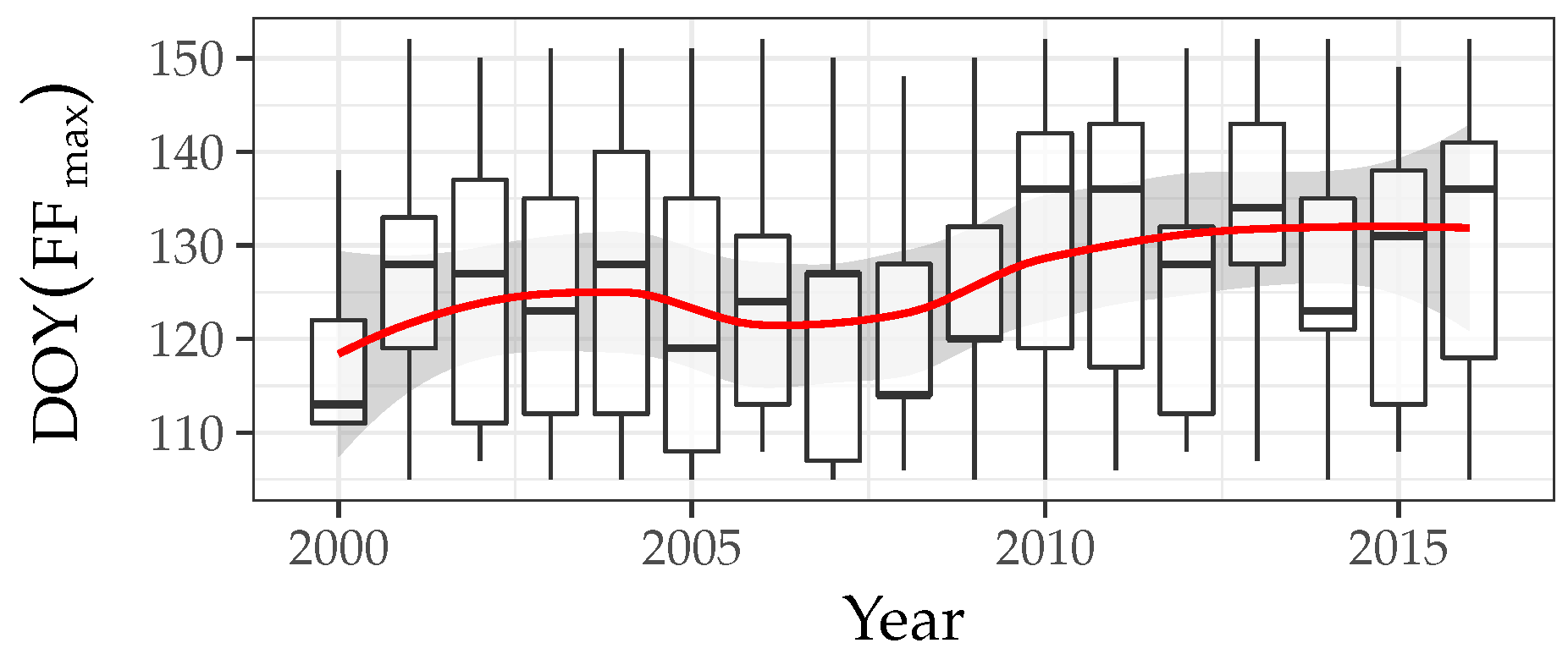
The analysis of the temporal changes of maximum FF occurrence (DOY(FFmax); see Section 2.4.3) highlighted a general delay throughout the whole rice district. The DOY of maximum flooding extent changed from about 120–130 (first ten days of May) during 2000–2009 to about 130–140 (mid-May) in the last seven years (Figure 4); the univariate linear regression between DOY(FFmax) and year (Equation (7)) confirms a global change of 0.75 ± 0.31 days per year (t = 2.39, p-value = 0.03). As shown in 
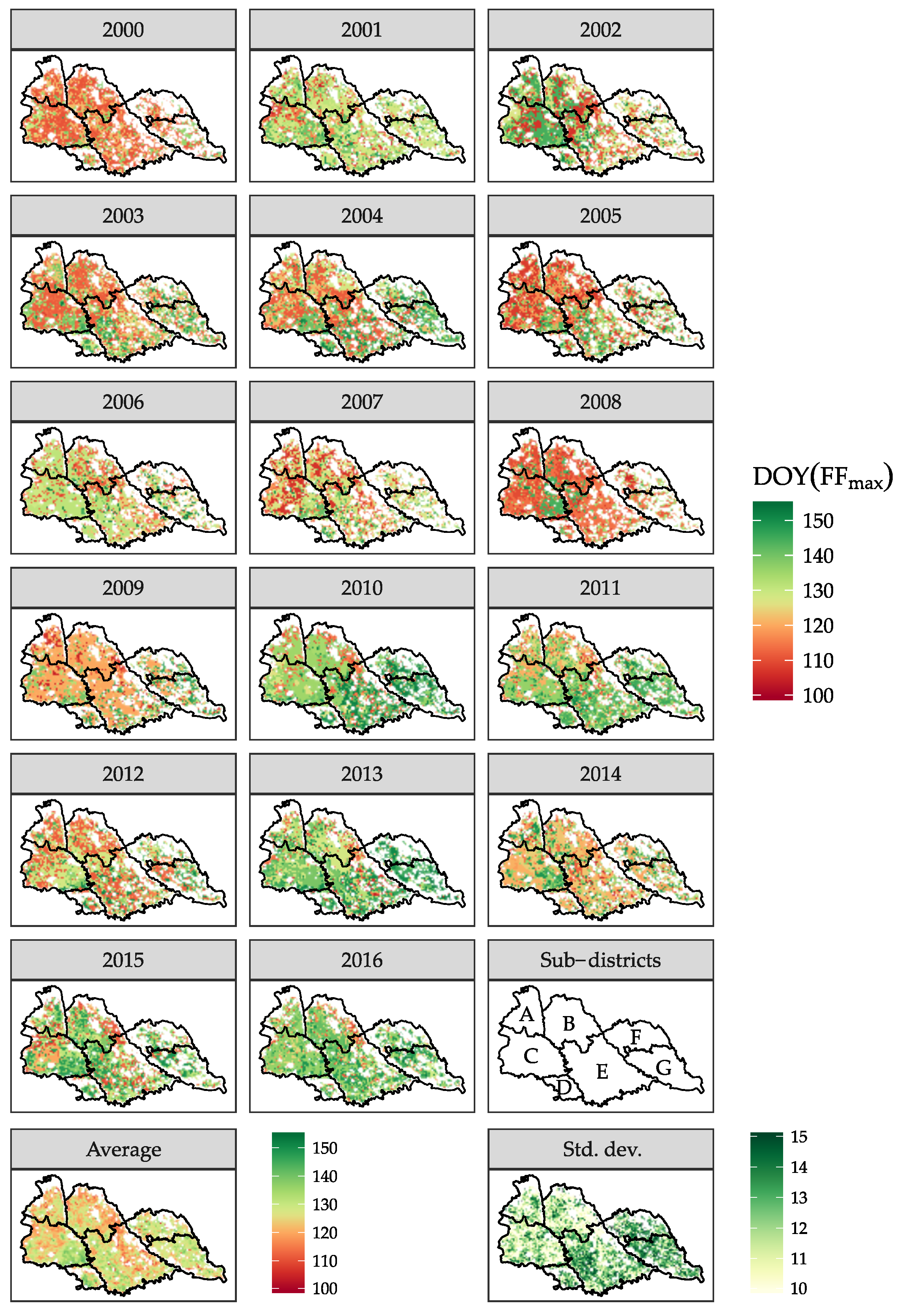
Figure 5, the flooding period in the northwestern sub-districts is generally slightly anticipated with respect to the southeastern ones (higher DOY value, although this is not evident in all years), consistent with the fact that northwestern sub-districts, being nearer to rivers, can be the first to receive water when it becomes available in spring. This is confirmed by the ANOVA (Table 2) of the multivariate regression (Equation (10)), which points out that most of the variance is explained by the “year” variable ( F = 28.29 ) and only slightly by the sub-district ( F = 2.61 ). No difference in the trend between sub-districts resulted from the analysis (interaction between year and sub-district: F = 0.29 , p-value = 0.94), even if the southeast ones revealed a slightly bigger change (Figure 5, panel of the standard deviation).

3.2. Analysis of the Spatial Distribution of Flooding Conditions

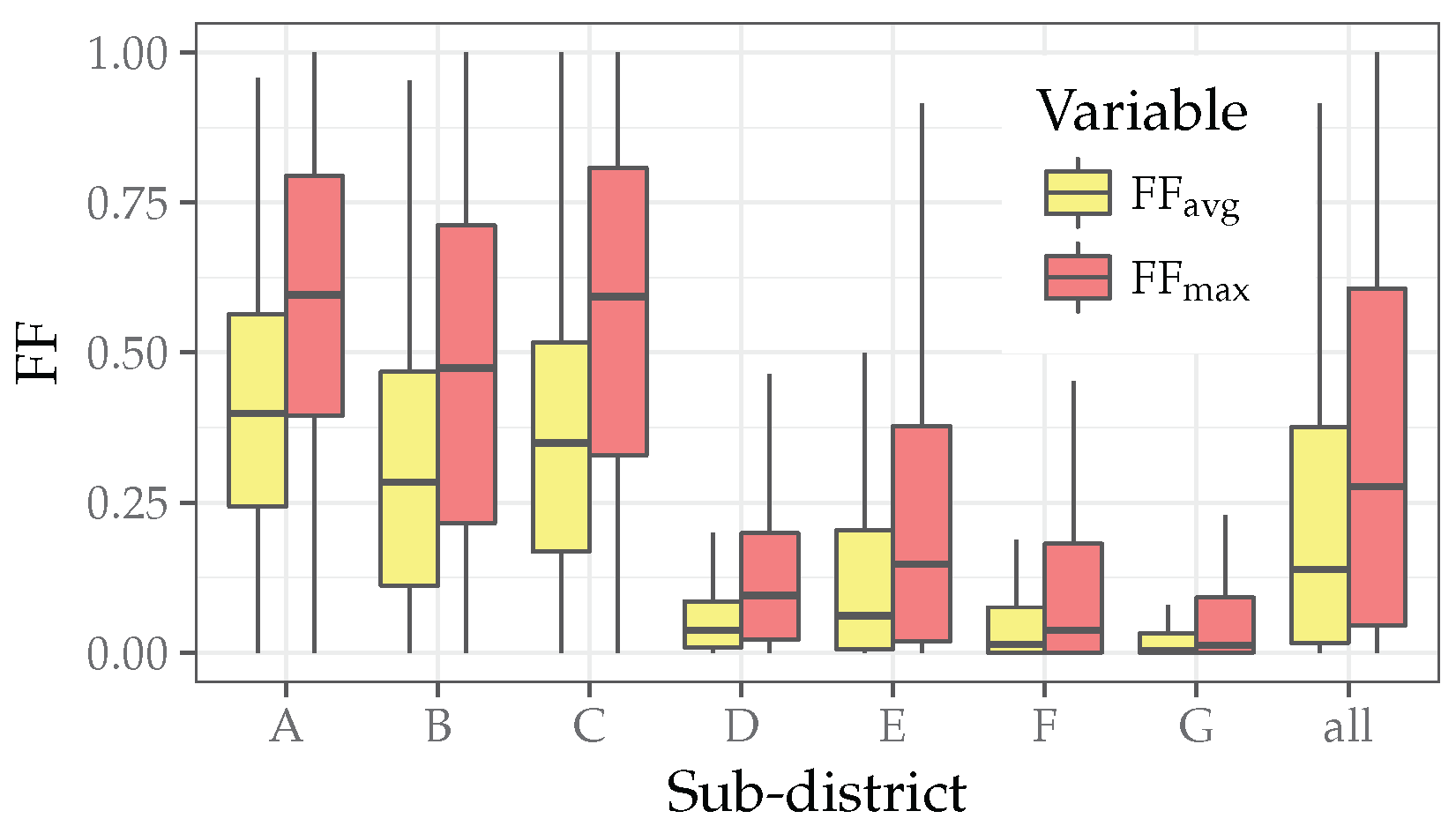
The spatial distribution of overall flooding conditions during the sowing phase (FFavg) was not uniform, with higher values detected in the northwestern parts of the study area than in the southeastern one.
This difference is also highlighted by Figure 6, where two groups of sub-districts can be easily identified. While in the entire rice district FFavg and FFmax, the averages are 0.22 and 0.35, respectively, the values between Sub-districts A-B-C (northwestern part, FF avg = 0.34 and FF max = 0.53 ) and D-E-F-G (southeastern part, FF avg = 0.10 and FF max = 0.18 ) differ considerably.
This is due to various causes, among which: (i) the proportion of rice-cultivated area, which is considerably higher in the northwestern parts, leading to higher FFavg (see Table 1); (ii) the greater and earlier adoption of dry seeding in the eastern part, leading to lower FFmax values. Considering the altitudinal gradient of this area, which decreases from northwest to southeast, it is also evident how the averaged flooding fraction decreases from the higher, northwestern sub-districts towards the lower, southeastern ones, in accordance with our knowledge about the geographical distribution of water availability in the study area. Northwestern sub-districts, being nearer to rivers, have higher water availability with respect to the southeastern ones. This probably led to a greater spread of dry seeding in the southeastern sub-districts, as already pointed out in Ranghetti et al. [
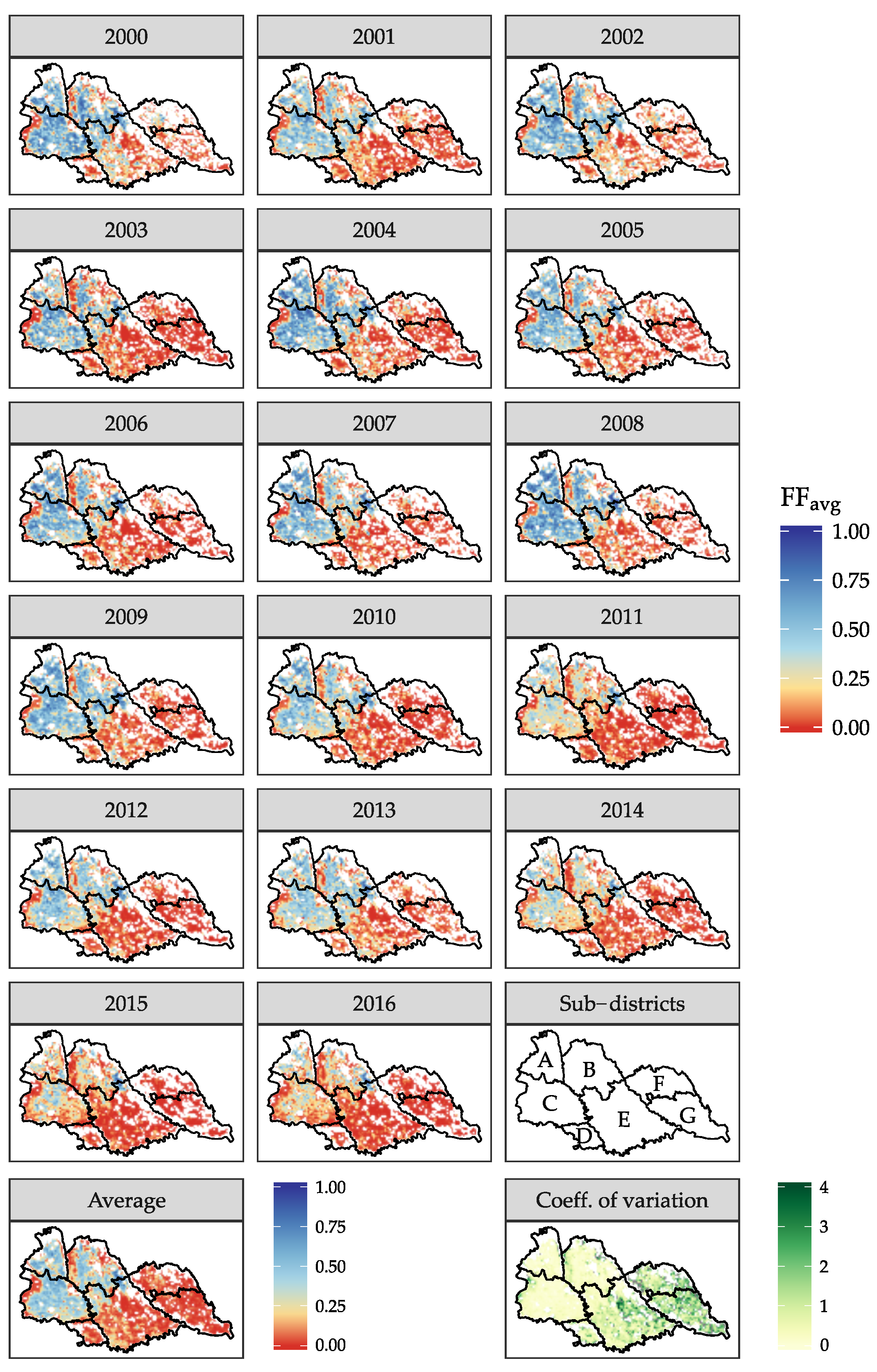
52]. The map of the coefficient of variation of seasonal FFavg values (Figure 7, last panel) also highlights that the interannual variation of standing water presence is higher in the eastern sub-districts, where water is less available.
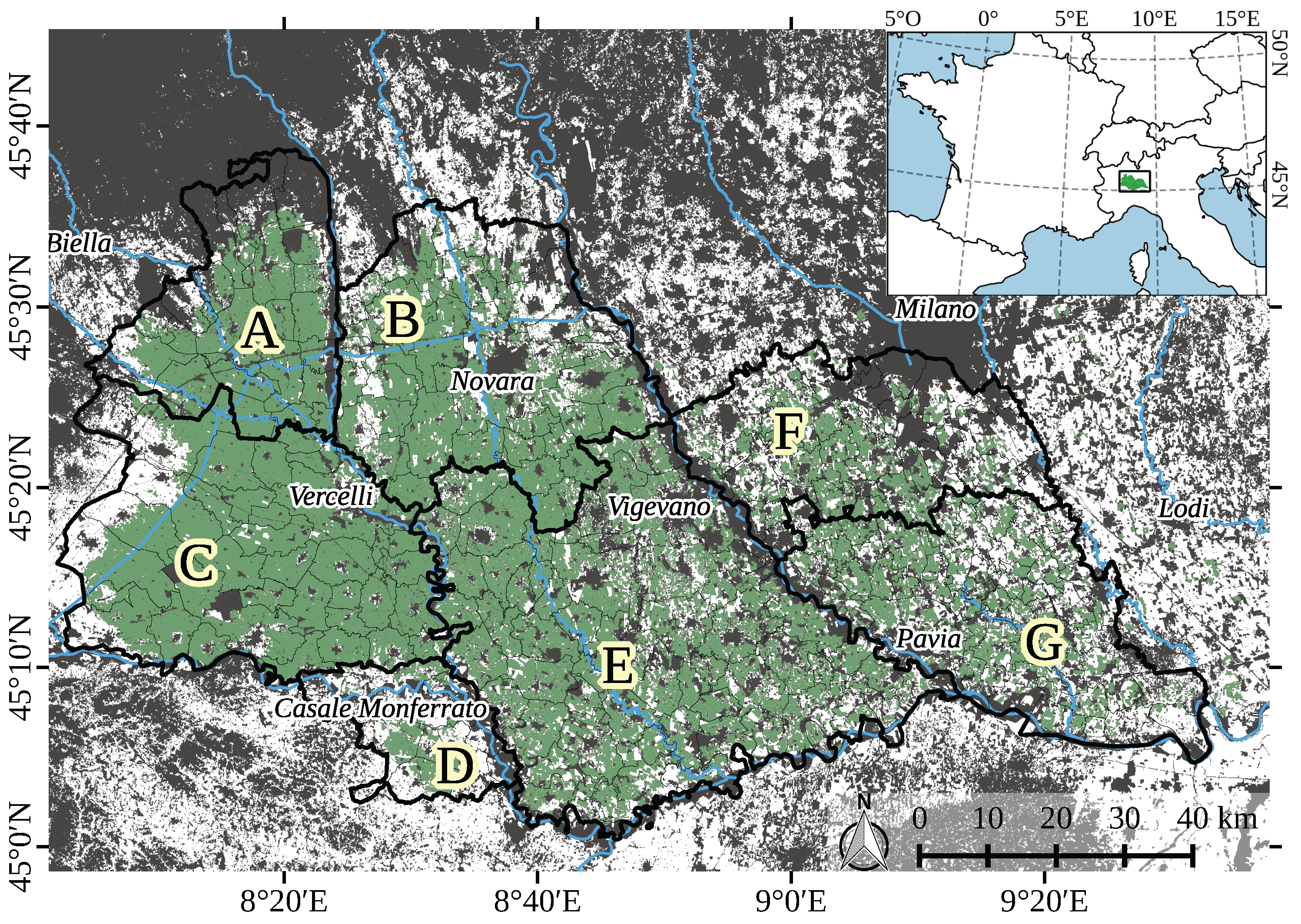
Figure 7 finally highlights that Sub-district E (Lomellina) exhibits differences between its northwestern (higher flooding fractions), northeastern (lower values) and southern (intermediate values) parts. This is due to differences in crop fractional cover (rice is dominant in the northwestern and southern parts, while in the northeastern one, other spring crops prevail) and rice practices (water availability is higher in the northwestern part, particularly in the area between Vigevano and Trecate), which make this sub-district fairly heterogeneous. Nevertheless, it was considered as a unique sub-district to simplify interpretation of the results aggregated on administrative boundaries.

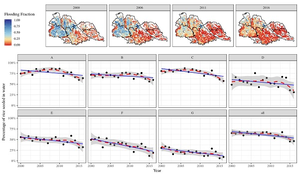
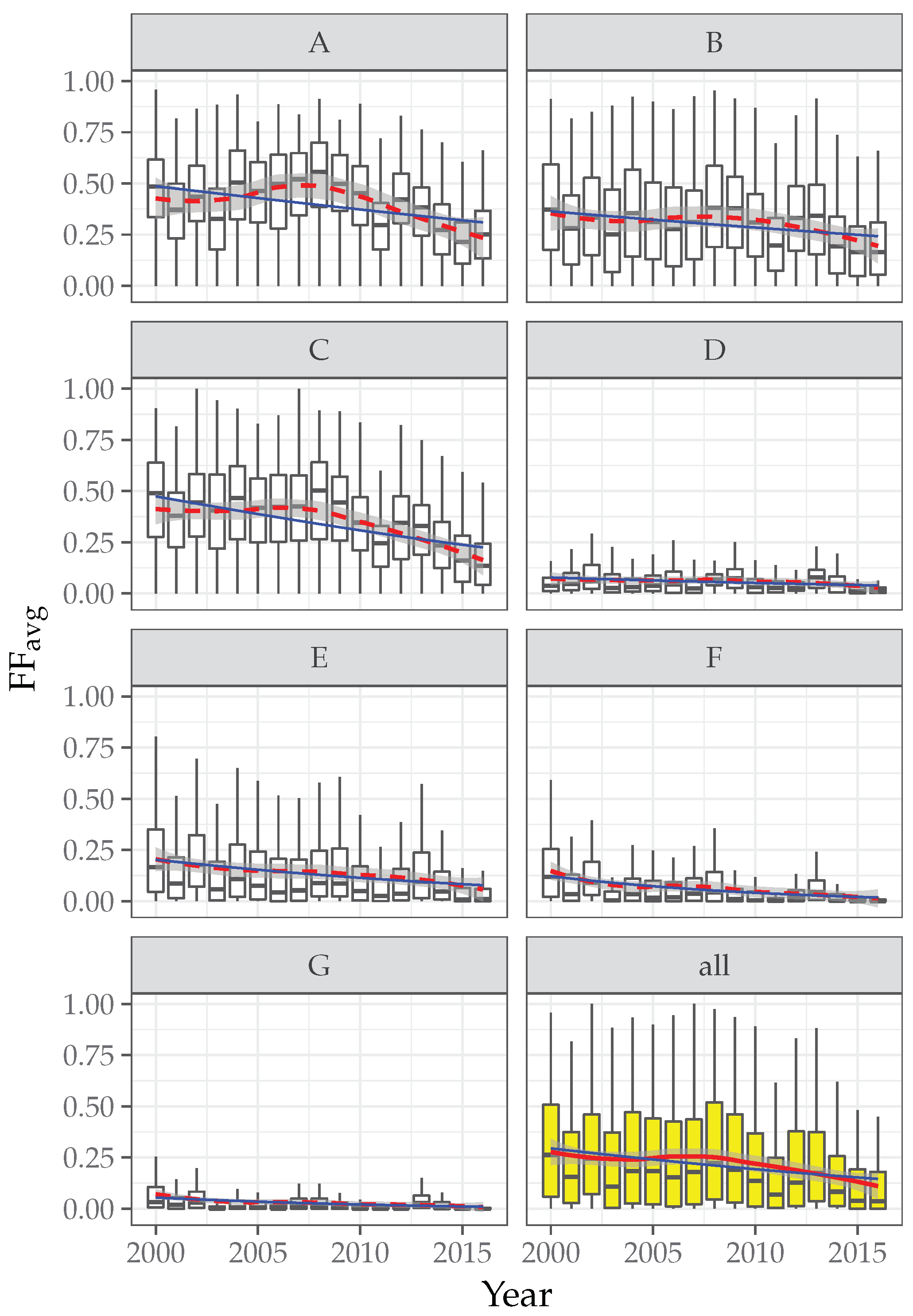
3.3. Analysis of Temporal Trends in Flooding Conditions in 2000–2016

The temporal analysis of the seasonal average Flooding Fraction (FFavg) allows identifying and quantifying a decreasing trend in overall flooding conditions during the sowing period (both globally and within each sub-district), as well as identifying differences between sub-districts.
When the whole rice district is considered, the univariate linear regression between FFavg and year (Equation (8)) shows a decrease of 0.86 ± 0.20 % per year ( t = 4.33 , p-value = 0.00059). This metric confirms that flooding practice, hence water diffusion, has been steadily decreasing within the study area.
Results of the ANOVA analysis, reported in Table 3, allow ascertaining the effect and significance of the different factors (years and sub-districts) and of their interaction. Although most of the variance is explained by the sub-districts (an expected result considering the differences in rice cover and irrigation regimes among sub-districts; see Figure 6), the effect of year is highly significant. This confirms that the decrease in flooding occurrence highlighted by the previous univariate regression analysis is a common pattern for all sub-districts and was not conveyed by the effect of averaging values from different sub-districts.
The significant sub-district × year interaction, even if low, also suggests that the rate of FFavg decrease varied between sub-districts. This is however influenced by the fact that southeastern sub-districts are characterized by a generally lower FFavg: the slope of the trend line can therefore be expected to be lower even if a similar relative interannual decrease is observed.
Results of the regression analysis conducted at the sub-district level (Figure 8 and Table 4) confirm that sub-districts can be split into two groups according to their mean flooding fraction, as already pointed out in the descriptive analysis. In the first group (Districts A, B and C, i.e., the northwestern ones) FFavg were considerably greater than in the second group (Districts D, E, F and G, i.e., the southeastern part), in accordance with the large amount of variance explained by the sub-district predictor in the multivariate regression (12). Table 3 also highlights the presence of a statistically-significant decreasing trend for all of the sub-districts. In summary, even if overall flooding conditions are spatially heterogeneous, their decreasing trend is widespread over the whole rice cultivation area, with a minimum decrease of 0.21 ± 0.09 % per year in Sub-district D and a maximum decrease of 1.46 ± 0.28 % per year in Sub-district C.
Values of FFmax multiplied by the rice area of each sub-district can be used to quantify the surface that was flooded at least once per year during sowing, a measure that can be considered a proxy of the water-seeded area (Table 5). Estimated flooded surface has reduced from 2000–2016 in all sub-districts, with a global reduction of 44% and a reduction within sub-districts varying from 24% in Sub-district A to 80% in Sub-district G. This finding is particularly interesting from an ecological point of view: the higher relative flooding decrease, i.e., the loss of foraging habitats for herons and egrets, appears in fact to be located within the eastern sub-districts where also landscape fragmentation is more pronounced, with a potential combined negative effect for waterbird populations.

3.4. Relationships between Raw WS Data and Official Statistics

Results of the logistic regression analysis (see Section 2.4.2) showed that the estimates of the proportion of water-seeded rice fields within each sub-district obtained from FFmax (WSraw) are highly correlated ( R 2 = 0.94 ) with Ente Nazionale Risi official data (WSENR) for the period 2004–2015 (Figure 9). Thanks to this finding, it was possible to use the resulting regression equation as a means to calibrate the WSraw estimates, thus allowing one to provide unbiased seasonal WS estimates for the different sub-districts for the whole analyzed time period.
WSraw resulted in being quite underestimated with respect to ENR statistics, likely because a single pixel can contain several paddy fields (more than 20, as the area of one pixel is 86 ha, while rice paddies have an average size of 3 ha [52]). Therefore, if paddies included in a single pixel are not flooded simultaneously, FFmax may underestimate the fraction of paddies flooded at least once during sowing. In fact, being F j ( t ) the flooding status (zero for dry, one for flooded) of a single paddy j ( j { 1 , , m } ) in a composite image t ( t { 1 , , n } ), the real maximum total extent of flooded surface during sowing should be computed as:
FF max = j = 1 m max t [ n ] F j ( t )
while FFmax was computed as:
FF max = max t [ n ] j = 1 m F j ( t )
where j = 1 m F j ( t ) = FF ( t ) , connecting Equation (16) to Equation (3). From this different computation method, it follows that FF max FF max on all possible conditions.
However, FF max is not directly calculable from input 1 × 1 km maps, since single paddies are not discernible; this consideration justifies the use of an empirical correction of WSraw values to balance the observed bias between FFmax and FF max .
ENR statistics were essential to obtain unbiased WS measures. Nevertheless, the possibility to estimate this variable from satellite data rather than from farmer declarations is important for several reasons: (i) remote sensing provides impartial and spatialized measures, while a map of the paddies is needed to compute the surface area of declared water- and dry-seeded fields (in this case, the area of cadastral parcels was used, which is often not updated and does not correspond to the actual extent of farming parcels); (ii) remote sensing data allow performing retrospective analysis up to early 2000, hence extending the temporal span of the trend analysis; (iii) estimations from remote data can be automatically updated every year (this will allow further extension of the analysis of the detected changes in the future, without requiring additional field/official data); (iv) the satellite-based estimation can be provided earlier in the season instead of waiting for the collection of farmers declaration, since input MODIS products are freely available two weeks after they are collected by the sensor. In conclusion, satellite data allow providing a near-real-time seasonal view of the water extent and easily broaden the analysis of the flooding condition trends in future years.

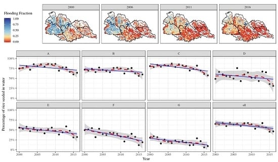
3.5. Analysis of Changes in the Proportion of Water-Seeded Area

The analysis conducted on the temporal variations of the estimated proportion of Water-Seeded rice (WS) (globally and among sub-districts) provided results quite similar to the ones described for FFavg trends, but with some interesting differences in terms of changes over time.
Results of the ANOVA analysis on the proportion of water-seeded rice fields (Table 6) show that, similarly to what was observed for FFavg, the sub-district is the most important factor in explaining WS variance, but year also has a statistically-significant effect. However, differently from what was observed for FFavg, the interaction between district and year is not statistically significant ( F = 1.19 , p-value = 0.32).
The univariate linear regression over years showed a significant WS decreasing trend of 0.91 ± 0.28 % per year ( t = 3.27 , p-value = 0.0051). This decrease is similar to that of FFavg ( 0.86 ± 0.20 % per year) and corresponds to a reduction of 14.6 ± 4.5 % ( 376.8 ± 1.6 km2) throughout the whole study period. The analysis within sub-districts (see Table 7 and Figure 10) shows that, also in the case of WS, a general decreasing trend is observed in all sub-districts, although some are not statistically significant (i.e., Sub-districts A, B and D).
However, comparing slope coefficients reported in Table 4 and Table 7, it can be observed that, while in the case of FFavg, the greater decrease occurred in the northwestern sub-districts, in the case of WS, the situation is the opposite. This apparent contradiction is justified by the fact that the slope of FFavg reduction depends also on the different rice fractional cover. A similar relative reduction of FFavg leads in fact to a larger slope of the regression for sub-districts characterized by a higher FFavg at the beginning of the period (as in the northwestern sub-district). WS trends do not present this problem and make it possible to analyze the relative variation of the water use within actual rice-cultivated areas directly.
Figure 10 also shows that in Sub-districts A, B and C, the decreasing trend is clearly not constant. The smoothed trends (red dashed lines) show in fact that a marked reduction of WS is evident only in the later years (i.e., 2009 onwards), while in the first ten years, no particular trends are evident. On the contrary, Sub-districts E, F and G show constant decreasing trends, as underlined by the almost coincident smoothed and linear trends.
Moreover, WS values in the first years of the analyzed period are close to one in Sub-districts A, B and C, while they are already close to 0.5 in the other ones (D, E and F), or even lower (G).
This evidence suggests that the lower decrease ratio of WS proportion in the northwestern sub-districts is due to a delayed adoption of the dry seeding practice. Further investigations on WS trends during future years are certainly needed to confirm this qualitative finding and to monitor if the WS proportion reduction will progress in the northwestern area with the same intensity already detected for the southeastern one.
It is also interesting to highlight the anomalous behavior of 2013 in all sub-districts (more evident in the southern ones). This is due to the atypically strong and continuous spring rain occurred during sowing in that year [79], which forced farmers to sow rice in flooded conditions. This finding is confirmed by ENR statistics (see also Figure 1 of Ranghetti et al. [52]).
Monitoring the trends of FFavg in the next few years will be crucial both to: (i) detect cases of extreme reduction of flooded surfaces in the southeastern sub-districts (east of the Ticino river), where the flooding extent is already low and a further reduction could lead to a critical shrinking of feeding habitats for herons and egrets; and (ii) prevent that the spread of dry seeding in northwestern sub-districts reaches the intensities already observed on the southeastern ones.
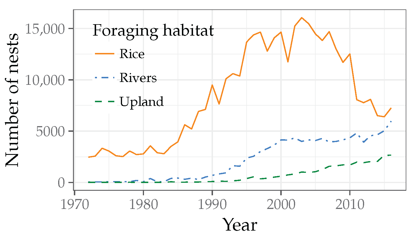
Comparing Figure 10 (panel “all”) with Figure 1 suggests in fact that the temporal trend of flooded surfaces could be associated with the observed reduction in the population size of waterbirds. The number of nests within rice fields (orange line in Figure 1) showed a decrease between 2000 and 2016 and, similarly to what was observed for WS, which decreased speeded-up since 2010. Nevertheless, in order to understand if there is indeed a causality between the reduction of water-seeded rice area and the number of nests, it would be necessary to study the population dynamics of herons and egrets in combination with other environmental and biological factors. This topic is currently under investigation, and the results of the present study are among the bulk of data under analysis.

4. Conclusions

This study applied a method to estimate the Flooding Fraction (FF) from MODIS data [52] with the aim to investigate the spatial and temporal trend of flooding within rice fields in the Italian rice district from 2000–2016. Results highlighted that the seasonal averaged flood intensity (FFavg) and the proportion of water-seeded rice-cultivated area (WS) decreased by 0.86 ± 0.20 % and 0.91 ± 0.28 % per year, respectively. Moreover, the seasonality of flooding events within the rice-sowing period changed, with a delay in the date of maximum flooding of 0.75 ± 0.31 days per year, suggests a modification in agro-practices and/or cultivated varieties. These changes were found to be widespread throughout the study area, but with strong differences among sub-districts for both FFavg and WS. Analysis of WS trends showed that the spread of dry seeding was already in progress in 2000 in the southeastern parts of the rice district, while it began only recently (about 2009) in the northwestern ones.
During the study period, the rice-cropped area was not reduced, so that the diminution of the standing water areas is to be attributed to the adoption of dry seeding. According to the described results, the adoption of this technique produced a loss of 44 % in the surface of paddies where herons and egrets could forage compared to 2000. The loss is greater in the southeastern part of the rice district, reaching up to 76 % and 80 % in the two eastern sub-districts. Such a reduction may explain the decreasing trend of heron and egret populations observed in the last few years.
These results, and those of concomitant studies on the foraging ecology of the breeding herons and egrets [54,80], will be used in order to assess the effect of environmental and biological factors involved in the recent decrease of these waterbirds.
To limit the massive spread of rice dry seeding, the 2014–2020 Common Agricultural Policy (CAP) already adopted redistributive payments for farmers who implement ecological mitigation (Action 214). This can be done both in Piedmont (Sub-districts A, B, C and D), where Actions 8.2.9.3.2 of the local Programma di Sviluppo Rurale (rural development program) [81] provide support for an anticipated stropping of droughts and for maintaining a partial flooded surface within drought paddies, and in Lombardy (Sub-districts E, F and G), where the attention is focused on the creation of a ditch along each paddy [82] (see Action 10.1.c) to maintain a minimum water reserve without losing efficiency in water management.

Acknowledgments

We wish to thank Bruno Marabelli from Ente Nazionale Risi for providing us unpublished data about sowing practices in the Italian rice district (Section 2.3). We are grateful to the NASA/MODIS Land Discipline Group and to the U.S. Geological Survey for producing and sharing of the MODIS dataset. This project was partially supported by the European Union’s Seventh Framework Programme for research, technological development and demonstration (FP7 2007-2013, ERMESproject, Grant Agreement No. 606983) and by the Italian Ministry of Education, University and Research (PRIN 2010–2011, 20108 TZKHC).

Author Contributions

M.F., M.B. and L.R. conceived of and designed the experiments. L.R. analyzed the data and wrote the paper. M.F. and E.C. wrote the ecological aspects in the paper. L.B. and M.B. reviewed the data analysis. M.B., M.F., E.C. and L.B. reviewed the paper.

Conflicts of Interest

The authors declare no conflict of interest.

Abbreviations

The following abbreviations are used in this manuscript:
ANOVAANalysis Of VAriance
DOYDay Of the Year
ENRItalian Ente Nazionale Risi
FFFlooding Fraction
FFavgAveraged Flooding Fraction value in the sowing season
FFmaxMaximum Flooding Fraction value in the sowing season
MODISMODerate-resolution Imaging Spectroradiometer
NDFINormalized Difference Flood Index
NDVINormalized Difference Vegetation Index
WSProportion of cultivated area of water-seeded rice during each year

References

  1. Tilman, D.; May, R.; Lehman, C.; Nowak, M. Habitat destruction and the extinction debt. Nature 1994, 371, 65–66. [Google Scholar] [CrossRef]
  2. Dudgeon, D.; Arthington, A.; Gessner, M.; Kawabata, Z.I.; Knowler, D.; Lévêque, C.; Naiman, R.; Prieur-Richard, A.H.; Soto, D.; Stiassny, M.; et al. Freshwater biodiversity: Importance, threats, status and conservation challenges. Biol. Rev. Camb. Philos. Soc. 2006, 81, 163–182. [Google Scholar] [CrossRef] [PubMed]
  3. Sala, O.; Chapin, F., III; Armesto, J.; Berlow, E.; Bloomfield, J.; Dirzo, R.; Huber-Sanwald, E.; Huenneke, L.; Jackson, R.; Kinzig, A.; et al. Global biodiversity scenarios for the year 2100. Science 2000, 287, 1770–1774. [Google Scholar] [CrossRef] [PubMed]
  4. Finlayson, C.M.; Hollis, T.; Dacis, T.; Crivelli, A. Managing Mediterranean Wetlands and Their Birds; IWRB: Slimbridge, UK, 1992.
  5. Fasola, M.; Ruiz, X. The value of rice fields as substitutes for natural wetlands for waterbirds in the Mediterranean Region. Waterbirds 1996, 19, 122–128. [Google Scholar] [CrossRef]
  6. Elphick, C.; Oring, L. Winter management of Californian rice fields for waterbirds. J. Appl. Ecol. 1998, 35, 95–108. [Google Scholar] [CrossRef]
  7. Elphick, C. Functional equivalency between rice fields and seminatural wetland habitats. Conserv. Biol. 2000, 14, 181–191. [Google Scholar] [CrossRef]
  8. Maeda, T. Patterns of bird abundance and habitat use in rice fields of the Kanto Plain, central Japan. Ecol. Res. 2001, 16, 569–585. [Google Scholar] [CrossRef]
  9. Tourenq, C.; Bennetts, R.; Kowalski, H.; Vialet, E.; Lucchesi, J.L.; Kayser, Y.; Isenmann, P. Are ricefields a good alternative to natural marshes for waterbird communities in the Camargue, southern France? Biol. Conserv. 2001, 100, 335–343. [Google Scholar] [CrossRef]
  10. Czech, H.; Parsons, K. Agricultural wetlands and waterbirds: A review. Waterbirds 2002, 25, 56–65. [Google Scholar]
  11. Ma, Z.; Li, B.; Zhao, B.; Jing, K.; Tang, S.; Chen, J. Are artificial wetlands good alternatives to natural wetlands for waterbirds?—A case study on Chongming Island, China. Biodivers. Conserv. 2004, 13, 333–350. [Google Scholar] [CrossRef]
  12. Sánchez-Guzmán, J.; Morán, R.; Masero, J.; Corbacho, C.; Costillo, E.; Villegas, A.; Santiago-Quesada, F. Identifying new buffer areas for conserving waterbirds in the Mediterranean basin: The importance of the rice fields in Extremadura, Spain. Biodivers. Conserv. 2007, 16, 3333–3344. [Google Scholar] [CrossRef]
  13. Toral, G.; Figuerola, J. Unraveling the importance of rice fields for waterbird populations in Europe. Biodivers. Conserv. 2010, 19, 3459–3469. [Google Scholar] [CrossRef]
  14. Ente Nazionale Risi. XLVIII Relazione Annuale Anno 2015; Ente Nazionale Risi: Milan, Italy, 2016. [Google Scholar]
  15. FAOSTAT. Production Crop; Food and Agriculture Organization of the United Nations: Rome, Italy, 2013. [Google Scholar]
  16. Romani, M. Tecnica colturale. In Il Riso; Bayer CropScience: Milan, Italy, 2008. [Google Scholar]
  17. De Maria, S.C.; Bischetti, G.; Chiaradia, E.; Facchi, A.; Miniotti, E.; Rienzner, M.; Romani, M.; Tenni, D.; Gandolfi, C. The role of water management and environmental factors on field irrigation requirements and water productivity of rice. Irrig. Sci. 2017, 35, 11–26. [Google Scholar] [CrossRef]
  18. Dunn, B.; Gaydon, D. Rice growth, yield and water productivity responses to irrigation scheduling prior to the delayed application of continuous flooding in south-east Australia. Agric. Water Manag. 2011, 98, 1799–1807. [Google Scholar] [CrossRef]
  19. Kato, Y.; Okami, M.; Katsura, K. Yield potential and water use efficiency of aerobic rice (Oryza sativa L.) in Japan. Field Crops Res. 2009, 113, 328–334. [Google Scholar] [CrossRef]
  20. Hill, J.; Buyer, D.; Bocchi, S.; Clampett, W. Direct seeded rice in the temperate climates of Australia, Italy, and the United States. In Proceedings of the Direct Seeded Flooded Rice in the Tropics: Selected Papers from the International Rice Research Conference, Seoul, Korea, 27–31 August 1990; International Rice Research Institute and Korea (South), Nongchon Chinhungchong, Ed.; International Rice Research Institute: Los Baños, Philippines, 1991; pp. 91–102. [Google Scholar]
  21. Fasola, M.; Rubolini, D.; Merli, E.; Boncompagni, E.; Bressan, U. Long-term trends of heron and egret populations in Italy, and the effects of climate, human-induced mortality, and habitat on population dynamics. Popul. Ecol. 2010, 52, 59–72. [Google Scholar] [CrossRef]
  22. Fasola, M.; Boncompagni, E. Il Monitoraggio delle Garzaie nel 2016—Quarantacinquesimo Anno. 2017. Available online: http://ecoeto.unipv.it/component/jdownloads/finish/37-documenti/160-relazionegarzaie2016 (accessed on 23 November 2017).
  23. Imperio, S.; Ranghetti, L.; von Hardenberg, J.; Provenzale, A.; Boncompagni, E.; Fasola, M. Effects of protection status, climate, and water management of rice felds on longterm population dynamics of herons and egrets in north-western Italy. In Proceedings of the 6th Symposium for Research in Protected Areas, Salzburg, Austria, 2–3 November 2017. [Google Scholar]
  24. Regione Piemonte. Piano Direttore Regionale per L’approvvigionamento Idropotabile e l’uso Integrato delle Risorse Idriche, Finalizzato al Risanamento, al Risparmio, Alla Tutela, Alla Riqualificazione e All’utilizzo a Scopo Multiplo delle Acque in Piemonte; Regione Piemonte: Turin, Italy, 2000. [Google Scholar]
  25. Facchi, A.; Gharsallah, O.; Chiaradia, E.; Bischetti, G.; Gandolfi, C. Monitoring and Modelling Evapotranspiration in Flooded and Aerobic Rice Fields. Procedia Environ. Sci. 2013, 19, 794–803. [Google Scholar] [CrossRef]
  26. Miniotti, E.; Romani, M.; Said-Pullicino, D.; Facchi, A.; Bertora, C.; Peyron, M.; Sacco, D.; Bischetti, G.; Lerda, C.; Tenni, D.; et al. Agro-environmental sustainability of different water management practices in temperate rice agro-ecosystems. Agric. Ecosyst. Environ. 2016, 222, 235–248. [Google Scholar] [CrossRef]
  27. Rahman, M.; Di, L. The state of the art of spaceborne remote sensing in flood management. Nat. Hazards 2017, 85, 1223–1248. [Google Scholar] [CrossRef]
  28. U.S. Geological Survey. Landsat; USGS/Earth Resources Observation and Science (EROS) Center: Sioux Falls, SD, USA, 2016.
  29. Frazier, P.; Page, K. Water body detection and delineation with Landsat TM data. Photogramm. Eng. Remote Sens. 2000, 66, 1461–1467. [Google Scholar]
  30. Du, Z.; Linghu, B.; Ling, F.; Li, W.; Tian, W.; Wang, H.; Gui, Y.; Sun, B.; Zhang, X. Estimating surface water area changes using time-series Landsat data in the Qingjiang River Basin, China. J. Appl. Remote Sens. 2012, 6, 063609. [Google Scholar] [CrossRef]
  31. Chormanski, J.; Okruszko, T.; Ignar, S.; Batelaan, O.; Rebel, K.; Wassen, M. Flood mapping with remote sensing and hydrochemistry: A new method to distinguish the origin of flood water during floods. Ecol. Eng. 2011, 37, 1334–1349. [Google Scholar] [CrossRef]
  32. Ouma, Y.; Tateishi, R. A water index for rapid mapping of shoreline changes of five East African Rift Valley lakes: An empirical analysis using Landsat TM and ETM+ data. Int. J. Remote Sens. 2006, 27, 3153–3181. [Google Scholar] [CrossRef]
  33. Tulbure, M.; Broich, M. Spatiotemporal dynamic of surface water bodies using Landsat time-series data from 1999 to 2011. ISPRS J. Photogramm. Remote Sens. 2013, 79, 44–52. [Google Scholar] [CrossRef]
  34. Feyisa, G.; Meilby, H.; Fensholt, R.; Proud, S. Automated Water Extraction Index: A new technique for surface water mapping using Landsat imagery. Remote Sens. Environ. 2014, 140, 23–35. [Google Scholar] [CrossRef]
  35. Rokni, K.; Ahmad, A.; Selamat, A.; Hazini, S. Water feature extraction and change detection using multitemporal landsat imagery. Remote Sens. 2014, 6, 4173–4189. [Google Scholar] [CrossRef]
  36. Hassani, M.; Chabou, M.; Hamoudi, M.; Guettouche, M. Index of extraction of water surfaces from Landsat 7 ETM+ images. Arab. J. Geosci. 2015, 8, 3381–3389. [Google Scholar] [CrossRef]
  37. Lunetta, R.; Balogh, M. Application of multi-temporal Landsat 5 TM imagery for wetland identification. Photogramm. Eng. Remote Sens. 1999, 65, 1303–1310. [Google Scholar]
  38. Ozesmi, S.; Bauer, M. Satellite remote sensing of wetlands. Wetl. Ecol. Manag. 2002, 10, 381–402. [Google Scholar] [CrossRef]
  39. Kulawardhana, R.; Thenkabail, P.; Vithanage, J.; Biradar, C.; Islam, M.; Gunasinghe, S.; Alankara, R. Evaluation of the wetland mapping methods using Landsat ETM+ and SRTM data. J. Spat. Hydrol. 2007, 7, 62–96. [Google Scholar]
  40. Islam, M.; Thenkabail, P.; Kulawardhana, R.; Alankara, R.; Gunasinghe, S.; Edussriya, C.; Gunawardana, A. Semi-automated methods for mapping wetlands using Landsat ETM+ and SRTM data. Int. J. Remote Sens. 2008, 29, 7077–7106. [Google Scholar] [CrossRef]
  41. Brivio, P.; Colombo, R.; Maggi, M.; Tomasoni, R. Integration of remote sensing data and GIS for accurate mapping of flooded areas. Int. J. Remote Sens. 2002, 23, 429–441. [Google Scholar] [CrossRef]
  42. Copernicus Programme. Sentinel-2; Copernicus: Vincennes, France, 2016. [Google Scholar]
  43. Du, Y.; Zhang, Y.; Ling, F.; Wang, Q.; Li, W.; Li, X. Water bodies’ mapping from Sentinel-2 imagery with Modified Normalized Difference Water Index at 10-m spatial resolution produced by sharpening the swir band. Remote Sens. 2016, 8, 354. [Google Scholar] [CrossRef] [Green Version]
  44. Sylvain, F.; Yann, K.; Ahmad, A.B.; Page, M.; Adrien, S.; Stephane, M.; Alexandre, B.; Jean-Christophe, M.; Sat, T.; Muddu, S.; et al. Synergetic Use of Sentinel-1 and 2 to Improve Agro-Hydrological Modeling: Preliminary Results on Rice Paddy Detection in South-India; European Space Agency: Toulouse, France, 2016; Volume SP-740. [Google Scholar]
  45. Ferrant, S.; Selles, A.; Le Page, M.; Herrault, P.A.; Pelletier, C.; Al-Bitar, A.; Mermoz, S.; Gascoin, S.; Bouvet, A.; Saqalli, M.; et al. Detection of irrigated crops from Sentinel-1 and Sentinel-2 data to estimate seasonal groundwater use in South India. Remote Sens. 2017, 9, 1119. [Google Scholar] [CrossRef]
  46. Sakamoto, T.; Yokozawa, M.; Toritani, H.; Shibayama, M.; Ishitsuka, N.; Ohno, H. A crop phenology detection method using time-series MODIS data. Remote Sens. Environ. 2005, 96, 366–374. [Google Scholar] [CrossRef]
  47. Boschetti, M.; Stroppiana, D.; Brivio, P.; Bocchi, S. Multi-year monitoring of rice crop phenology through time series analysis of MODIS images. Int. J. Remote Sens. 2009, 30, 4643–4662. [Google Scholar] [CrossRef]
  48. Motohka, T.; Nasahara, K.; Miyata, A.; Mano, M.; Tsuchida, S. Evaluation of optical satellite remote sensing for rice paddy phenology in monsoon Asia using a continuous in situ dataset. Int. J. Remote Sens. 2009, 30, 4343–4357. [Google Scholar] [CrossRef]
  49. Peng, D.; Huete, A.; Huang, J.; Wang, F.; Sun, H. Detection and estimation of mixed paddy rice cropping patterns with MODIS data. Int. J. Appl. Earth Obs. Geoinf. 2011, 13, 13–23. [Google Scholar] [CrossRef]
  50. Tornos, L.; Huesca, M.; Dominguez, J.; Moyano, M.; Cicuendez, V.; Recuero, L.; Palacios-Orueta, A. Assessment of MODIS spectral indices for determining rice paddy agricultural practices and hydroperiod. ISPRS J. Photogramm. Remote Sens. 2015, 101, 110–124. [Google Scholar] [CrossRef]
  51. NASA LP DAAC. MODIS; USGS/Earth Resources Observation and Science (EROS) Center: Sioux Falls, SD, USA, 2014.
  52. Ranghetti, L.; Busetto, L.; Crema, A.; Fasola, M.; Cardarelli, E.; Boschetti, M. Testing estimation of water surface in Italian rice district from MODIS satellite data. Int. J. Appl. Earth Obs. Geoinf. 2016, 52, 284–295. [Google Scholar] [CrossRef]
  53. Boschetti, M.; Nutini, F.; Manfron, G.; Brivio, P.A.; Nelson, A. Comparative Analysis of Normalized Difference Spectral Indices Derived from MODIS for Detecting Surface Water in Flooded Rice Cropping Systems. PLoS ONE 2014, 9, e88741. [Google Scholar] [CrossRef] [PubMed]
  54. Fasola, M.; Cardarelli, E. Long-term changes in the food resources of a guild of breeding Ardeinae (Aves) in Italy. Ital. J. Zool. 2015, 82, 238–250. [Google Scholar] [CrossRef]
  55. Regione Lombardia. DUSAF, 4th ed.; Direzione Generale Territorio, Urbanistica e difesa del suolo, Regione Lombardia: Milano, Italy, 2014. [Google Scholar]
  56. Regione Piemonte. Land Cover Piemonte; Area SIT—Sistemi Informativi Territoriali: Torino, Italy, 2008. [Google Scholar]
  57. European Environment Agency. Corine Land Cover Raster Data, version 18.5; European Environment Agency: Copenhagen, Denmark, 2016. [Google Scholar]
  58. Vermote, E. MOD09A1 MODIS/Terra Surface Reflectance 8-Day L3 Global 500 m SIN Grid V006; NASA EOSDIS Land Processes DAAC: Washington, DC, USA, 2015.
  59. Tucker, C. Red and photographic infrared linear combinations for monitoring vegetation. Remote Sens. Environ. 1979, 8, 127–150. [Google Scholar] [CrossRef]
  60. Busetto, L.; Ranghetti, L. MODIStsp: An R package for preprocessing of MODIS Land Products time series. Comput. Geosci. 2016, 97, 40–48. [Google Scholar] [CrossRef]
  61. Busetto, L.; Ranghetti, L. MODIStsp: An R Package for Preprocessing of MODIS Time Series, R package version 1.3.3. 2017. Available online: https://cran.r-project.org/web/packages/MODIStsp/vignettes/MODIStsp.pdf (accessed on 23 November 2017).
  62. R Core Team. R: A Language and Environment for Statistical Computing; R Foundation for Statistical Computing: Vienna, Austria, 2017. [Google Scholar]
  63. Zambrano-Bigiarini, M. HydroGOF: Goodness-Of-Fit Functions for Comparison of Simulated and Observed Hydrological Time Series, R package version 0.3-8. 2014. Available online: https://mran.microsoft.com/snapshot/2014-11-17/web/packages/hydroGOF/hydroGOF.pdf (accessed on 23 November 2017).
  64. Canty, A.; Ripley, B. Boot: Bootstrap R (S-Plus) Functions, R package version 1.3-18. 2016. Available online: https://cran.r-project.org/src/contrib/Archive/boot/ (accessed on 23 November 2017).
  65. Fox, J.; Weisberg, S. An R Companion to Applied Regression, 2nd ed.; Sage: Thousand Oaks, CA, USA, 2011. [Google Scholar]
  66. Warmerdam, F. The Geospatial Data Abstraction Library. In Open Source Approaches in Spatial Data Handling; Brent Hall, G., Leahy, M.G., Eds.; Springer: Berlin/Heidelberg, Germany, 2008; pp. 87–104. [Google Scholar]
  67. QGIS Development Team. QGIS Geographic Information System; Open Source Geospatial Foundation. 2016. Available online: https://www.qgis.org/en/site/about/index.html# (accessed on 23 November 2017).
  68. Bivand, R.S.; Pebesma, E.; Gómez-Rubio, V. Applied Spatial Data Analysis with R, 2nd ed.; Springer: New York, NY, USA, 2013. [Google Scholar]
  69. Bivand, R.; Keitt, T.; Rowlingson, B. Rgdal: Bindings for the Geospatial Data Abstraction Library, R package version 1.2-4. 2016. Available online: https://cran.r-project.org/src/contrib/Archive/rgdal/ (accessed on 23 November 2017).
  70. Greenberg, J.A.; Mattiuzzi, M. GdalUtils: Wrappers for the Geospatial Data Abstraction Library (GDAL) Utilities, R package version 2.0.1.7. 2015. Available online: https://cran.r-project.org/web/packages/gdalUtils/index.html (accessed on 23 November 2017).
  71. Hijmans, R.J. Raster: Geographic Data Analysis and Modeling, R package version 2.5-8. 2016. Available online: https://cran.r-project.org/src/contrib/Archive/raster/ (accessed on 23 November 2017).
  72. Bivand, R.; Rundel, C. Rgeos: Interface to Geometry Engine—Open Source (GEOS), R package version 0.3-21. 2016. Available online: http://mars.bilkent.edu.tr/R/web/packages/rgeos/index.html (accessed on 23 November 2017).
  73. Dowle, M.; Srinivasan, A. Data.table: Extension of ‘Data.frame’, R package version 1.10.0. 2016. Available online: https://cran.r-project.org/src/contrib/Archive/data.table/ (accessed on 23 November 2017).
  74. Wickham, H. Ggplot2: Elegant Graphics for Data Analysis; Springer: New York, NY, USA, 2009. [Google Scholar]
  75. Auguie, B. GridExtra: Miscellaneous Functions for “Grid” Graphics, R package version 2.2.1. 2016. Available online: https://cran.r-project.org/src/contrib/Archive/gridExtra/ (accessed on 23 November 2017).
  76. Boschetti, M.; Busetto, L.; Manfron, G.; Laborte, A.; Asilo, S.; Pazhanivelan, S.; Nelson, A. PhenoRice: A method for automatic extraction of spatio-temporal information on rice crops using satellite data time series. Remote Sens. Environ. 2017, 194, 347–365. [Google Scholar] [CrossRef]
  77. Busetto, L.; Casteleyn, S.; Granell, C.; Pepe, M.; Barbieri, M.; Campos-Taberner, M.; Casa, R.; Collivignarelli, F.; Confalonieri, R.; Crema, A.; et al. Downstream Services for Rice Crop Monitoring in Europe: From Regional to Local Scale. IEEE J. Sel. Top. Appl. Earth Obs. Remote Sens. 2017, 10, 5423–5441. [Google Scholar] [CrossRef]
  78. Wilkinson, G.; Rogers, C. Symbolic description of factorial models for analysis of variance. J. Appl. Stat. 1973, 22, 392–399. [Google Scholar] [CrossRef]
  79. Camera di Commercio di Pavia. Analisi Trimestrale sui Prezzi e sul Mercato del Risone; Camera di Commercio di Pavia: Pavia, Italy, 2013. [Google Scholar]
  80. Fasola, M.; Cardarelli, E.; Pellitteri-Rosa, D.; Ranghetti, L. The recent decline of heron populations in Italy and the changes in rice cultivation practice. In Proceedings of the 25th International Ornithological Congress, Tokyo, Japan, 18–25 August 2014; Volume 13. [Google Scholar]
  81. Regione Piemonte. Programma di Sviluppo Rurale PSR 2014-2020; Regione Piemonte: Turin, Italy, 2015. [Google Scholar]
  82. Regione Lombardia. Adozione della Proposta di Programma di Sviluppo Rrurale 2014–2020 a Valere sulle Risorse del Fondo Europeo Agricolo per lo Sviluppo Rurale (FEASR) da Notificare alla Commissione Europea. Deliberazione n. X/2116; Regione Lombardia: Milano, Italy, 2014. [Google Scholar]
Figure 1. Total number of nests of the two most abundant breeding waterbirds, the grey heron and the little egret, in northwestern Italy during the time window analyzed in this study, compared to their predominant foraging habitat [22,23].
Remotesensing 10 00416 g001
Figure 2. Localization of the northwestern Italian rice district. The rice-cultivated surface is shown in green, while non-arable land is shown in grey; thick lines and letters denote the sub-districts identified for the analyses (see Table 1 for details); thin lines denote municipality boundaries.
Remotesensing 10 00416 g002
Figure 3. Seasonal NDVI (top panel) and FF (bottom panel) distribution of pixels of the MODIS images (2000–2016) grouped by DOY composite period. NDVI distributions include all the pixels (the red dashed line is the proportion of values with NDVI < 0.4), while FF distributions include only selected pixels (NDVI < 0.4). Yellow boxes (grey in the printed version) represent the composites selected for the analysis (see Section 2.4.1).
Remotesensing 10 00416 g003
Figure 4. Temporal distribution of DOY(FFmax) over the whole rice district, with smoothed line tendency.
Remotesensing 10 00416 g004
Figure 5. Top panels: seasonal DOY(FFmax) maps; bottom panels: 2000–2016 average (left) and standard deviation (right) maps.
Remotesensing 10 00416 g005
Figure 6. Distribution of seasonal FF aggregated values (values with NDVI < 0.4) during the entire 2000–2016 study period within each sub-district and the whole district.
Remotesensing 10 00416 g006
Figure 7. Top panels: yearly maps of average flooding presence FFavg maps; bottom panels: 2000–2016 average (left) and coefficient of variation (right) maps.
Remotesensing 10 00416 g007
Figure 8. Temporal distribution of FFavg pixel values along the year and sub-districts (panels “A” to “G”) or the whole district (panel “all”). Solid blue lines represent the linear regression of Equation (11), while red dashed lines are smoothed tendencies, both performed on sub-district-based averaged values.
Remotesensing 10 00416 g008
Figure 9. Logistic regression between WSENR and WSraw: calibration points, regression curve with 95% confidence interval, validation metrics and equation.
Remotesensing 10 00416 g009
Figure 10. Temporal distribution of WS values along year and sub-districts. Points are predicted values (Equation (12)); blue lines represent the linear trends (Table 7); while red dashed lines are smoothed tendencies.
Remotesensing 10 00416 g010
Table 1. Characteristics of the rice district and sub-districts. “Rice area” is the surface classified as “rice” in the Corine Land Cover images (see Section 2.2.1).
IDDescriptionIrrigation AreaElevationTotal AreaRice Area% Rice on Total Crop
ABaraggeBaraggia Biellese e Vercellese200 m442 km2 243 ± 8 km280%
BNovareseEst Sesia146 m750 km2 484 ± 2 km281%
CGrange vercellesiOvest Sesia144 m850 km2 622 ± 11 km284%
DOltrepo casaleseDestra Po Casalese107 m206 km2 38 ± 6 km227%
ELomellinaEst Sesia96 m1269 km2 758 ± 8 km277%
FSud MilanoEst Ticino Villoresi103 m525 km2 134 ± 6 km239%
GPaveseEst Ticino Villoresi77 m661 km2 298 ± 3 km261%
allRice district 113 m4704 km2 2581 ± 47 km272%
Table 2. ANOVA table (type II tests) of the multivariate linear regression (Equation (10)) of DOY ( FF max ) over years and sub-districts (with the interaction term).
Sum SqDfF ValuePr (>F)
year1356.10128.290.0000
sub-district751.7362.610.0211
year:sub-district83.2760.290.9408
residuals5033.22105
Table 3. ANOVA table (type II tests) of the multivariate linear regression (Equation (11)) of FF avg over years and sub-districts (with their multiplicative effect).
Sum SqDfF ValuePr (>F)
year0.15173.530.0000
sub-district2.436198.970.0000
year:sub-district0.0563.690.0023
residuals0.21105
Table 4. Summary of the univariate linear regressions of FFavg over years (each line refers to an independent regression). Intercepts refer to year = 2000 instead of year = 0 to be more intelligible. Stars beside p-values identify significant values (p-value < 0.05).
Sub-DistrictIntercept (2000)Slope (year)t-ValuePr (>(|t|)
A 0.482 ± 0.037 0.0104 ± 0.0039 −2.650.0182*
B 0.360 ± 0.024 0.0071 ± 0.0025 −2.830.0126*
C 0.463 ± 0.026 0.0146 ± 0.0028 −5.240.0001*
D 0.075 ± 0.008 0.0021 ± 0.0009 −2.440.0273*
E 0.194 ± 0.014 0.0073 ± 0.0015 −4.750.0003*
F 0.113 ± 0.013 0.0064 ± 0.0014 −4.690.0003*
G 0.053 ± 0.007 0.0028 ± 0.0007 −4.020.0011*
all 0.286 ± 0.019 0.0086 ± 0.0020 −4.330.0006*
Table 5. Quantification of the surface (in km2) of flooded surfaces over years and sub-districts.
YearABCDEFGall
200014927744010.9427339.7540.971231
200115425841518.7024742.3748.431185
200217229347015.7329246.6643.511333
200313923542613.6820519.7816.301055
200419131346712.9026944.3431.941329
200517427245211.2221827.5122.941178
200619025150423.9623625.1017.621248
20071672354198.9816831.5628.081058
200819430748415.6124231.0822.181295
200919031245717.8827428.1926.311306
201019429744112.0421021.3420.031195
201113021433511.8614910.8710.79862
20121592913739.0718421.5611.911051
201315930745119.1530128.2637.931303
201412021533318.1921220.4325.12943
20151001782636.661094.994.92668
20161131992375.391139.458.03685
Table 6. ANOVA table (type II tests) of the multivariate linear regression (Equation (12)) of WS over years and sub-districts (with their multiplicative effect).
Sum SqDfF ValuePr (>F)
year0.30151.100.0000
sub-district4.666132.710.0000
year:sub-district0.0461.190.3151
residuals0.61105
Table 7. Summary of the univariate linear regressions of WS over years (each line refers to an independent regression). Intercepts refer to year = 2000 instead of year = 0 to be more intelligible. Stars beside p-values identify significant values (p-value < 0.05).
Sub-DistrictIntercept (2000)Slope (year)t ValuePr (>(|t|)
A 0.83 ± 0.03 0.008 ± 0.004 −2.100.0530
B 0.74 ± 0.03 0.005 ± 0.003 −1.810.0905
C 0.86 ± 0.03 0.011 ± 0.003 −3.640.0024*
D 0.61 ± 0.05 0.008 ± 0.006 −1.410.1783
E 0.56 ± 0.03 0.010 ± 0.003 −2.930.0104*
F 0.52 ± 0.04 0.018 ± 0.004 −4.810.0002*
G 0.29 ± 0.03 0.011 ± 0.003 −3.500.0032*
all 0.69 ± 0.03 0.009 ± 0.003 −3.270.0051*

