Optimal, Recursive and Sub-Optimal Linear Solutions to Attitude Determination from Vector Observations for GNSS/Accelerometer/Magnetometer Orientation Measurement


Abstract
1. Introduction
- The main theory is based on our previous research contributions and is extended to linear arbitrary pairs vector measurements for GNSS/AM attitude application.
- Three estimators, i.e., the Optimal Linear Estimator of Quaternion (OLEQ), Recursive OLEQ (ROLEQ) and Sub-optimal OLEQ (SOLEQ), are derived. We also proposed acceleration techniques to make the algorithms faster.
- Simulations and real experiments are carried out, which verify the accuracy, flexibility, robustness and time consumption of various algorithms for GNSS/AM attitude determination. Detailed comparisons with representative methods demonstrate the superiority of the proposed OLEQs.
2. Fundamentals of the GNSS/AM System
3. Problem Formulation
Quaternion from a Single Sensor Observation
4. Optimal Linear Estimator of the Quaternion
4.1. Variant 1: Recursive-OLEQ
4.2. Variant 2: SOLEQ
4.2.1. Two-Vector Case
4.2.2. n-Vector Case
4.2.3. The Effect of Power Order
4.3. Discussion of OLEQs
5. Simulations and Experiments
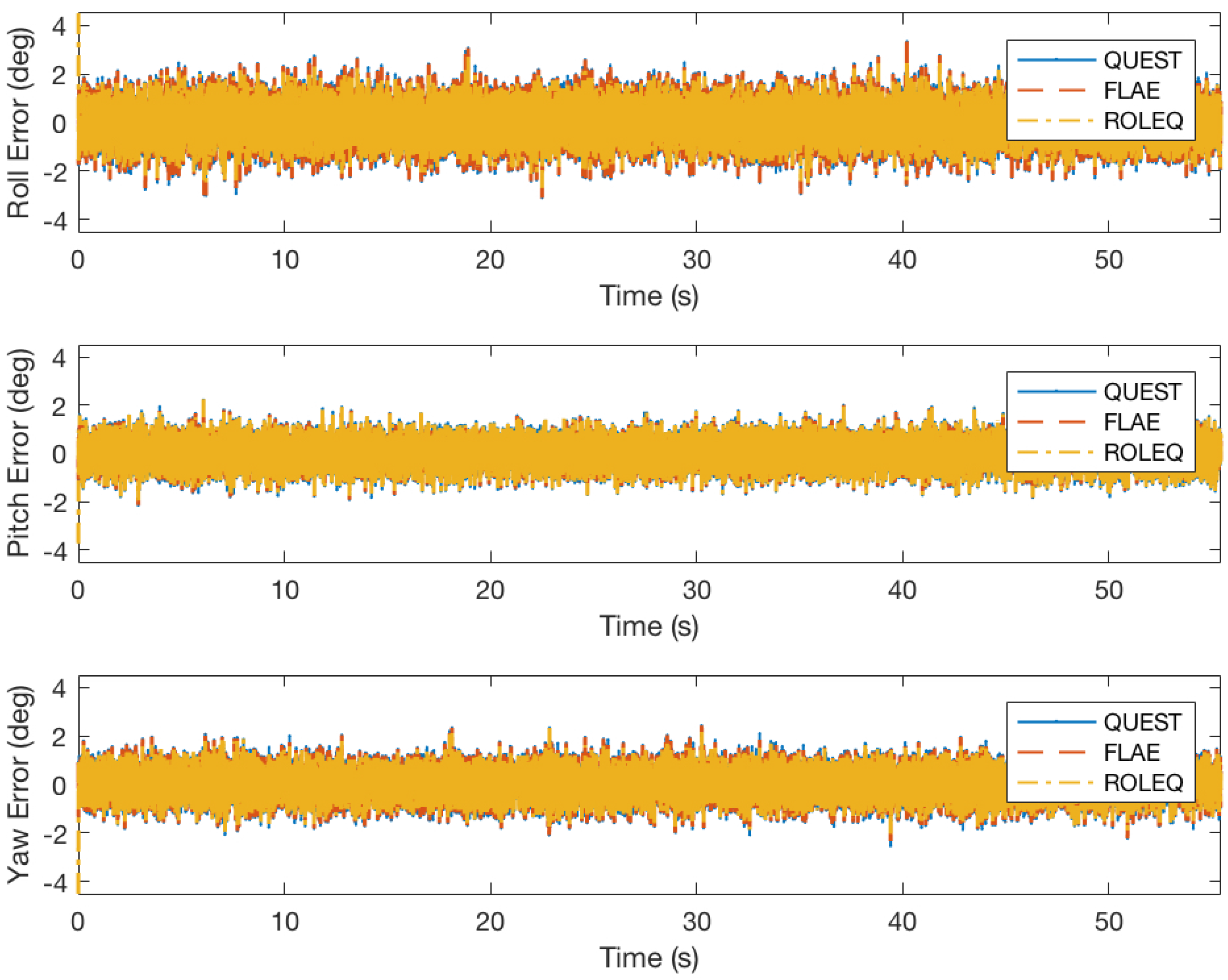
5.1. Simulation: Common Cases
5.2. Simulation: Extreme Cases
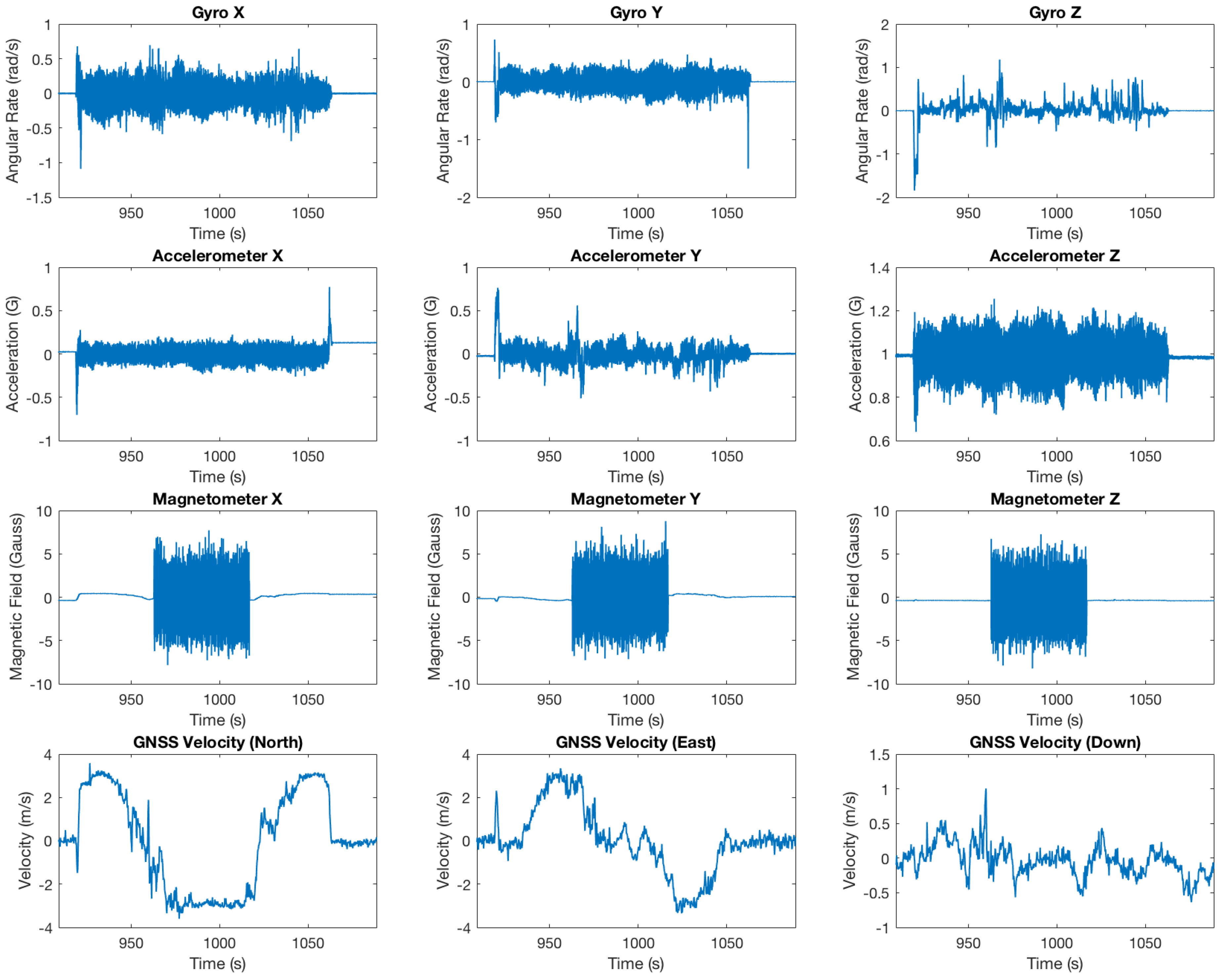
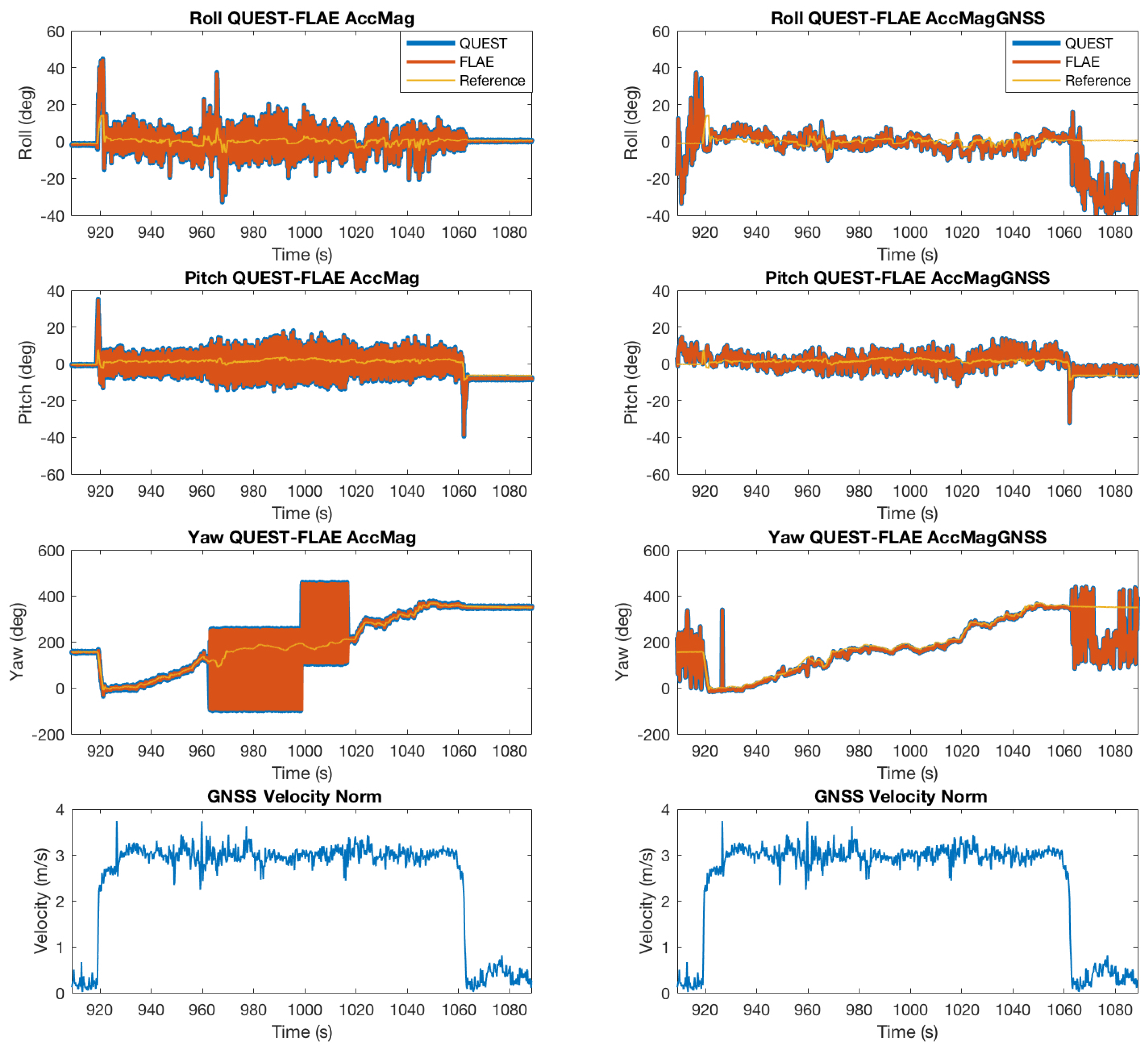
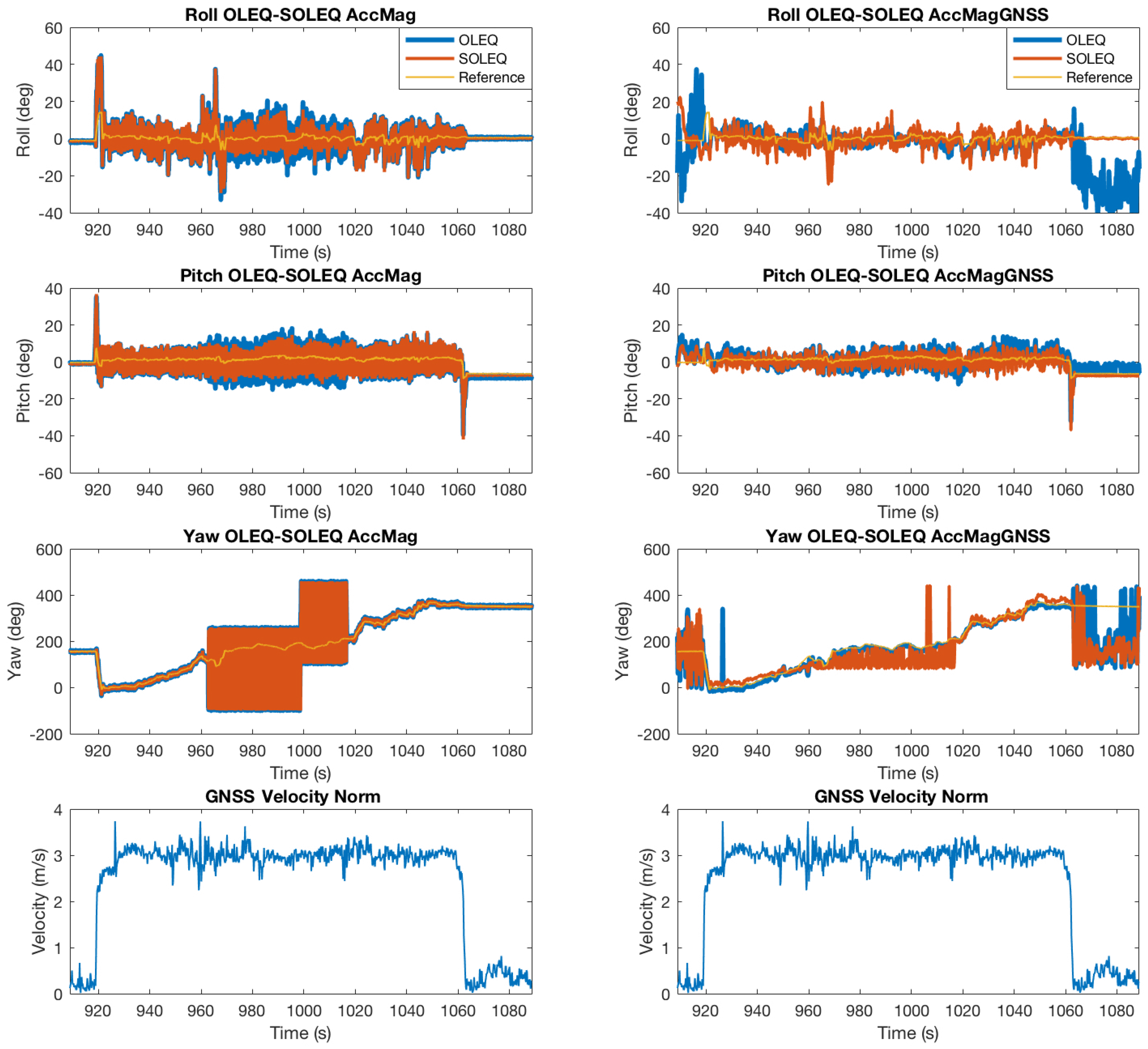
5.3. Experiment: Accelerometer-Magnetometer Case
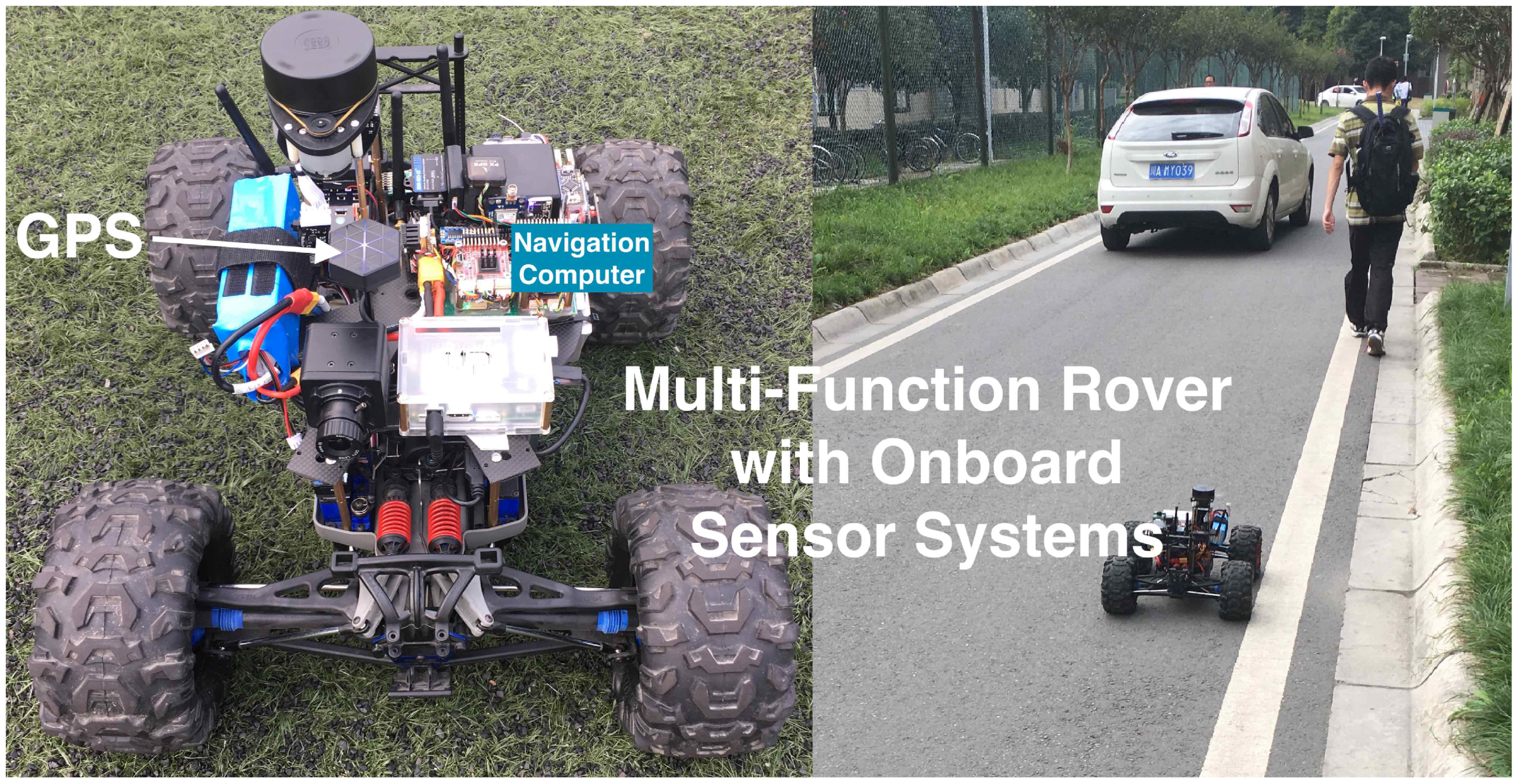
5.4. Experiment: GNSS-Aided Attitude Determination for Land Vehicles
5.5. Computation Time
6. Conclusions
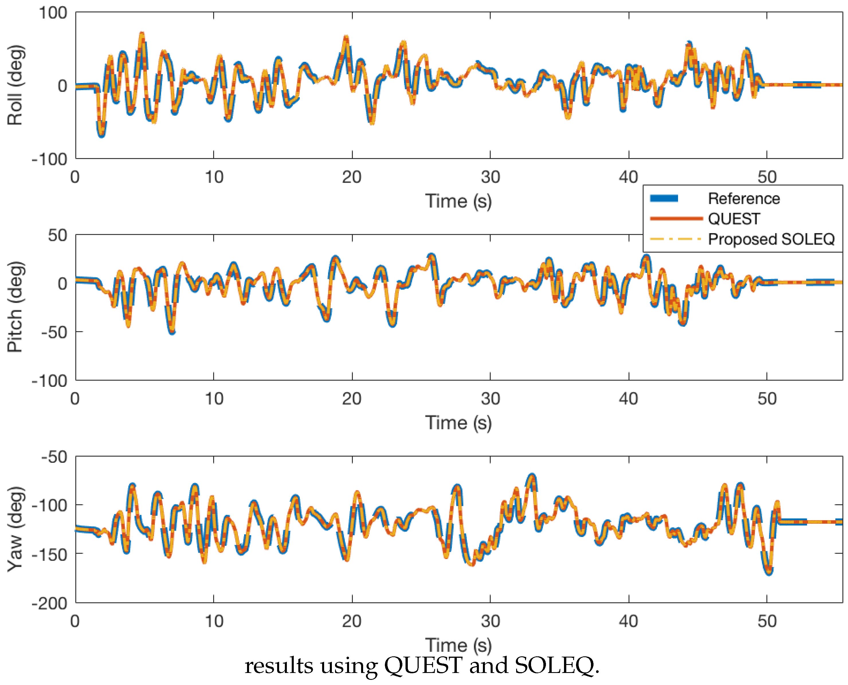
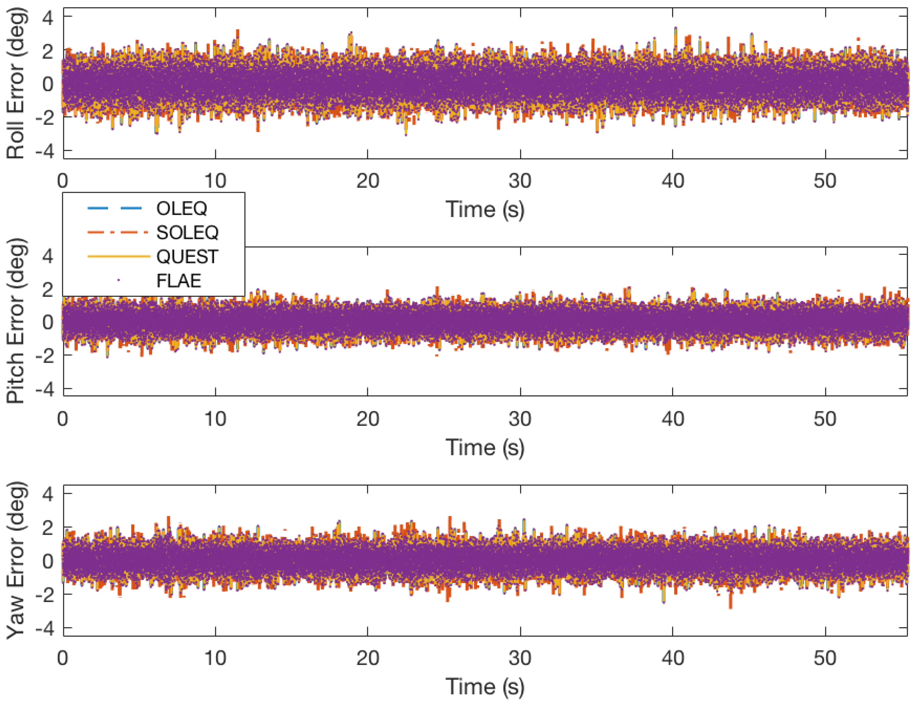
- Numerical simulations exhibit that the proposed OLEQs have a similar accuracy with representative solvers.
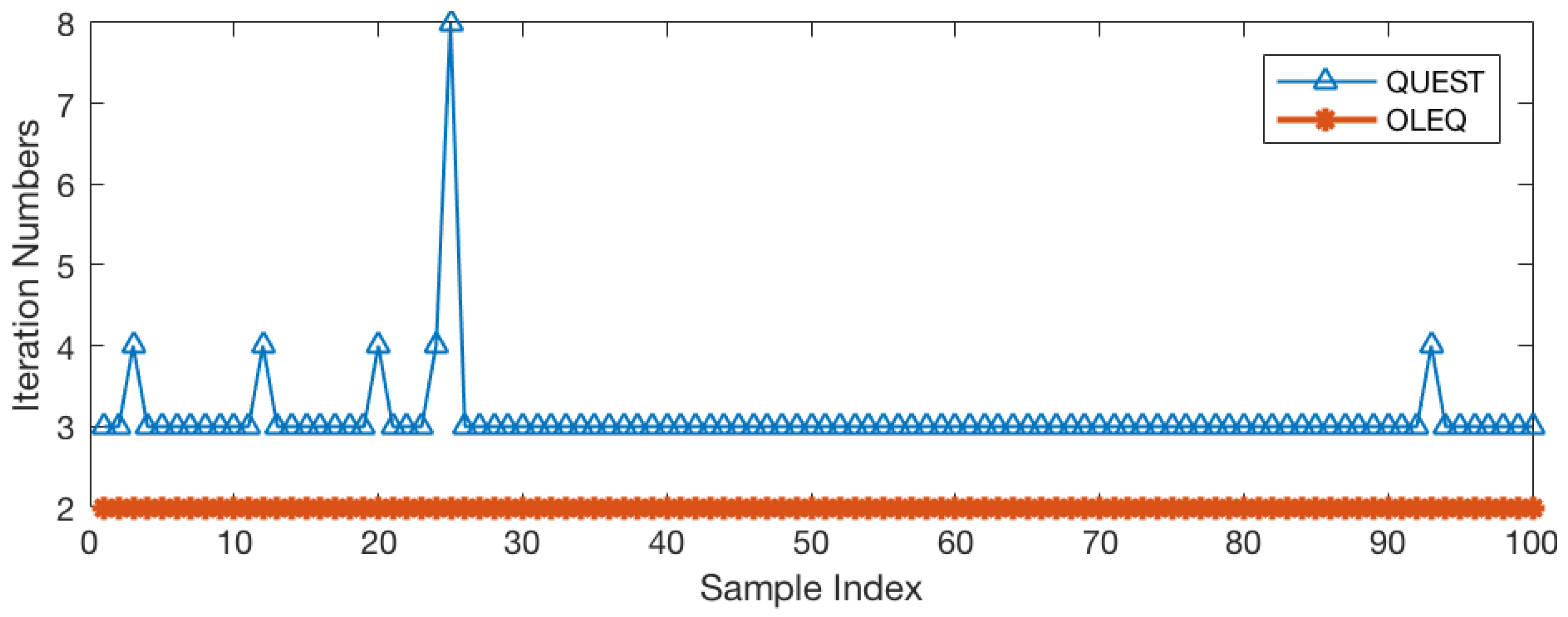
- It is also demonstrated that faced with extreme cases, OLEQs show much more robustness with less computation iterations.
- The computation speeds of OLEQs are tested, revealing that they belong to computationally-efficient algorithms.
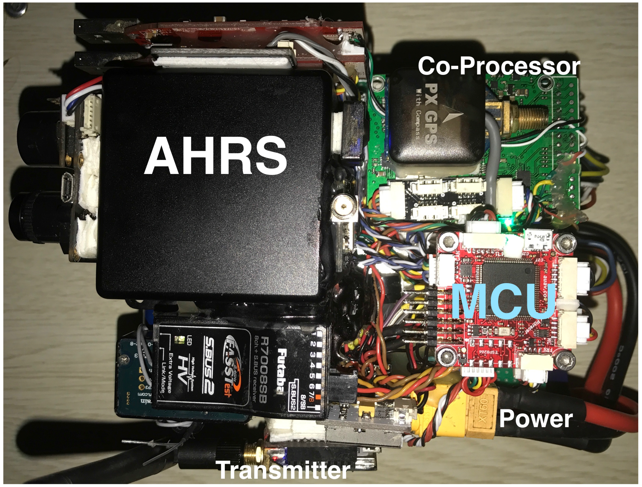
- Moreover, a real vehicular experiment of a GNSS/AM system is designed and conducted showing the effectiveness of the proposed OLEQs in real-world embedded applications.
Acknowledgments
Author Contributions
Conflicts of Interest
References
- Zhou, Z.; Li, Y.; Liu, J.; Li, G. Equality constrained robust measurement fusion for adaptive kalman-filter-based heterogeneous multi-sensor navigation. IEEE Trans. Aerosp. Electron. Syst. 2013, 49, 2146–2157. [Google Scholar]
- Zhou, Z.; Li, Y.; Zhang, J.; Rizos, C. Integrated Navigation System for a Low-Cost Quadrotor Aerial Vehicle in the Presence of Rotor Influences. J. Surv. Eng. 2017, 143, 05016006. [Google Scholar] [CrossRef]
- Chang, G.; Xu, T.; Wang, Q. M-estimator for the 3D symmetric Helmert coordinate transformation. J. Geod. 2017, 92, 47–58. [Google Scholar] [CrossRef]
- Wu, Y.; Wang, J.; Hu, D. A New Technique for INS/GNSS Attitude and Parameter Estimation Using Online Optimization. IEEE Trans. Signal Process. 2014, 62, 2642–2655. [Google Scholar] [CrossRef]
- Chang, L.; Qin, F.; Zha, F. Pseudo Open-Loop Unscented Quaternion Estimator for Attitude Estimation. IEEE Sens. J. 2016, 16, 4460–4469. [Google Scholar] [CrossRef]
- Han, S.; Wang, J. Quantization and colored noises error modeling for inertial sensors for GPS/INS integration. IEEE Sens. J. 2011, 11, 1493–1503. [Google Scholar] [CrossRef]
- Chang, L.; Li, J.; Chen, S. Initial Alignment by Attitude Estimation for Strapdown Inertial Navigation Systems. IEEE Trans. Instrum. Meas. 2015, 64, 784–794. [Google Scholar] [CrossRef]
- Marins, J.; Yun, X.; Bachmann, E.; McGhee, R.; Zyda, M. An extended Kalman filter for quaternion-based orientation estimation using MARG sensors. In Proceedings of the 2001 IEEE/RSJ International Conference on Intelligent Robots and Systems. Expanding the Societal Role of Robotics in the the Next Millennium (Cat. No.01CH37180), Maui, HI, USA, 29 October–3 November 2001; Volume 4. [Google Scholar]
- Tian, Y.; Wei, H.; Tan, J. An adaptive-gain complementary filter for real-time human motion tracking with MARG sensors in free-living environments. IEEE Trans. Neural Syst. Rehabil. Eng. 2013, 21, 254–264. [Google Scholar] [CrossRef] [PubMed]
- Wu, J.; Zhou, Z.; Li, R.; Yang, L.; Fourati, H. Attitude Determination Using a Single Sensor Observation : Analytic Quaternion Solutions and Property Discussion. IET Sci. Meas. Technol. 2017, 11, 731–739. [Google Scholar] [CrossRef]
- Du, S.; Gao, Y. Inertial aided cycle slip detection and identification for integrated PPP GPS and INS. Sensors 2012, 12, 14344–14362. [Google Scholar] [CrossRef] [PubMed]
- Aleshechkin, A. Algorithm of GNSS-based attitude determination. Gyroscopy Navig. 2011, 2, 269. [Google Scholar] [CrossRef]
- Grewal, M.; Andrews, A. Kalman Filtering: Theory and Practice Using MATLAB; John Wiley & Sons: Hoboken, NJ, USA, 2001. [Google Scholar]
- Niu, X.; Nassar, S.; El-Sheimy, N. An Accurate Land-Vehicle MEMS IMU/GPS Navigation System Using 3D Auxiliary Velocity Updates. Navigation 2007, 54, 177–188. [Google Scholar] [CrossRef]
- Niu, X.; Nasser, S.; Goodall, C.; El-Sheimy, N. A universal approach for processing any MEMS inertial sensor configuration for land-vehicle navigation. J. Navig. 2007, 60, 233–245. [Google Scholar] [CrossRef]
- Gebre-Egziabher, D.; Elkaim, G.H. MAV attitude determination by vector matching. IEEE Trans. Aerosp. Electron. Syst. 2008, 44. [Google Scholar] [CrossRef]
- Zhang, J.; Zhang, K.; Grenfell, R.; Deakin, R. Short note: On the relativistic Doppler effect for precise velocity determination using GPS. J. Geod. 2006, 80, 104–110. [Google Scholar] [CrossRef]
- Zhou, Z.; Li, B. Optimal Doppler-aided smoothing strategy for GNSS navigation. GPS Solut. 2017, 21, 197–210. [Google Scholar]
- Geng, J.; Bock, Y.; Melgar, D.; Crowell, B.W.; Haase, J.S. A new seismogeodetic approach applied to GPS and accelerometer observations of the 2012 Brawley seismic swarm: Implications for earthquake early warning. Geochem. Geophys. Geosyst. 2013, 14, 2124–2142. [Google Scholar] [CrossRef]
- Geng, J.; Melgar, D.; Bock, Y.; Pantoli, E.; Restrepo, J. Recovering coseismic point ground tilts from collocated high-rate GPS and accelerometers. Geophys. Res. Lett. 2013, 40, 5095–5100. [Google Scholar] [CrossRef]
- Wahba, G. A Least Squares Estimate of Satellite Attitude. SIAM Rev. 1965, 7, 409. [Google Scholar] [CrossRef]
- Shuster, M.D.; Oh, S.D. Three-axis attitude determination from vector observations. J. Guid. Control Dyn. 1981, 4, 70–77. [Google Scholar] [CrossRef]
- Markley, F.L. Attitude Determination using Vector Observations and the Singular Value Decomposition. J. Astronaut. Sci. 1988, 36, 245–258. [Google Scholar]
- Mortari, D. ESOQ: A Closed-Form Solution to the Wahba Problem. J. Astronaut. Sci. 1997, 45, 195–204. [Google Scholar]
- Davenport, P.B. A Vector Approach to the Algebra of Rotations with Applications; Technical Report August; National Aeronautics and Space Administration: Washington, DC, USA, 1968.
- Chang, G.; Xu, T.; Wang, Q. Error analysis of Davenport’s q method. Automatica 2017, 75, 217–220. [Google Scholar] [CrossRef]
- Wu, J.; Zhou, Z.; Gao, B.; Li, R.; Cheng, Y.; Fourati, H. Fast Linear Quaternion Attitude Estimator Using Vector Observations. IEEE Trans. Autom. Sci. Eng. 2018, 15, 307–319. [Google Scholar] [CrossRef]
- Yang, Y.; Zhou, Z. An analytic solution to Wahbas problem. Aerosp. Sci. Technol. 2013, 30, 46–49. Available online: http://xxx.lanl.gov/abs/1309.5679 (accessed on 24 February 2018). [CrossRef]
- Yang, Y. Attitude determination using Newton’s method on Riemannian manifold. Proc. Inst. Mech. Eng. Part G J. Aerosp. Eng. 2015, 229, 2737–2742. [Google Scholar] [CrossRef]
- Forbes, J.R.; de Ruiter, A.H.J. Linear-Matrix-Inequality-Based Solution to Wahba’s Problem. J. Guid. Control Dyn. 2015, 38, 147–151. [Google Scholar]
- Mahony, R.; Hamel, T.; Pflimlin, J.M. Nonlinear complementary filters on the special orthogonal group. IEEE Trans. Autom. Control 2008, 53, 1203–1218. [Google Scholar] [CrossRef]
- Madgwick, S.O.H.; Harrison, A.J.L.; Vaidyanathan, R. Estimation of IMU and MARG orientation using a gradient descent algorithm. In Proceedings of the IEEE International Conference on Rehabilitation Robotics, Zurich, Switzerland, 29 June–1 July 2011. [Google Scholar]
- Arun, K.S.; Huang, T.S.; Blostein, S.D. Least-Squares Fitting of Two 3-D Point Sets. IEEE Trans. Pattern Anal. Mach. Intell. 1987, PAMI-9, 698–700. [Google Scholar] [CrossRef]
- Ye, C.; Hong, S.; Tamjidi, A. 6-DOF Pose Estimation of a Robotic Navigation Aid by Tracking Visual and Geometric Features. IEEE Trans. Autom. Sci. Eng. 2015, 12, 1169–1180. [Google Scholar] [CrossRef] [PubMed]
- Abdelrahman, M.; Park, S.Y. Simultaneous spacecraft attitude and orbit estimation using magnetic field vector measurements. Aerosp. Sci. Technol. 2011, 15, 653–669. [Google Scholar] [CrossRef]
- Markley, F.L.; Mortari, D. Quaternion attitude estimation using vector observations. J. Astronaut. Sci. 2000, 48, 359–380. [Google Scholar]
- Markley, F.L.; Mortari, D. How to estimate attitude from vector observations. Adv. Astronaut. Sci. 2000, 103, 1979–1996. [Google Scholar]
- Markley, F.L. Humble problems. Adv. Astronaut. Sci. 2006, 124 II, 2205–2222. [Google Scholar]
- Wu, J.; Zhou, Z.; Chen, J.; Fourati, H.; Li, R. Fast Complementary Filter for Attitude Estimation Using Low-Cost MARG Sensors. IEEE Sens. J. 2016, 16, 6997–7007. [Google Scholar] [CrossRef]
- Shuster, M.D. Filter QUEST or REQUEST. J. Guid. Control Dyn. 2009, 32, 643–645. [Google Scholar] [CrossRef]
- Valenti, R.G.; Dryanovski, I.; Xiao, J. A Linear Kalman Filter for MARG Orientation Estimation Using the Algebraic Quaternion Algorithm. IEEE Trans. Instrum. Meas. 2016, 65, 467–481. [Google Scholar] [CrossRef]
- Horn, R.A.; Johnson, C.R. Matrix Analysis; Cambridge University Press: Cambridge, UK, 2012. [Google Scholar]
- Yang, Y. Spacecraft attitude determination and control: Quaternion based method. Annu. Rev. Control 2012, 36, 198–219. [Google Scholar] [CrossRef]
- Cheng, Y.; Shuster, M.D. Improvement to the Implementation of the QUEST Algorithm. J. Guid. Control Dyn. 2014, 37, 301–305. [Google Scholar] [CrossRef]
- Wu, Y.; Shi, W. On Calibration of Three-Axis Magnetometer. IEEE Sens. J. 2015, 15, 6424–6431. [Google Scholar] [CrossRef]


| Case | Reference Vectors | Noise Standard Deviations |
|---|---|---|
| 1 | ||
| 2 | ||
| 3 | ||
| 4 | ||
| 5 | ||
| 6 | ||
| 7 | ||
| 8 | ||
| 9 | ||
| 10 | ||
| 11 | ||
| 12 |
| Case | OLEQ | SOLEQ | QUEST | FLAE |
|---|---|---|---|---|
| 1 | ||||
| 2 | ||||
| 3 | ||||
| 4 | ||||
| 5 | ||||
| 6 | ||||
| 7 | ||||
| 8 | ||||
| 9 | ||||
| 10 | ||||
| 11 | ||||
| 12 |
| Case | OLEQ | SOLEQ | QUEST | FLAE |
|---|---|---|---|---|
| 1 | ||||
| 2 | ||||
| 3 | ||||
| 4 | ||||
| 5 | ||||
| 6 | ||||
| 7 | ||||
| 8 | ||||
| 9 | ||||
| 10 | ||||
| 11 | ||||
| 12 |
| Case | OLEQ | SOLEQ | QUEST | FLAE |
|---|---|---|---|---|
| 1 | ||||
| 2 | ||||
| 3 | ||||
| 4 | ||||
| 5 | ||||
| 6 | ||||
| 7 | ||||
| 8 | ||||
| 9 | ||||
| 10 | ||||
| 11 | ||||
| 12 |
| Case | OLEQ | SOLEQ | QUEST | FLAE |
|---|---|---|---|---|
| 1 | ||||
| 2 | ||||
| 3 | ||||
| 4 | ||||
| 5 | ||||
| 6 | ||||
| 7 | ||||
| 8 | ||||
| 9 | ||||
| 10 | ||||
| 11 | ||||
| 12 |
| Roll Case | OLEQ | SOLEQ | QUEST | FLAE |
| Acc-MagExperiment | ||||
| Acc-Mag-GNSS Experiment | ||||
| Pitch Case | OLEQ | SOLEQ | QUEST | FLAE |
| Acc-Mag Experiment | ||||
| Acc-Mag-GNSS Experiment | ||||
| Yaw Case | OLEQ | SOLEQ | QUEST | FLAE |
| Acc-Mag Experiment | ||||
| Acc-Mag-GNSS Experiment |
© 2018 by the authors. Licensee MDPI, Basel, Switzerland. This article is an open access article distributed under the terms and conditions of the Creative Commons Attribution (CC BY) license (http://creativecommons.org/licenses/by/4.0/).
Share and Cite
Zhou, Z.; Wu, J.; Wang, J.; Fourati, H. Optimal, Recursive and Sub-Optimal Linear Solutions to Attitude Determination from Vector Observations for GNSS/Accelerometer/Magnetometer Orientation Measurement. Remote Sens. 2018, 10, 377. https://doi.org/10.3390/rs10030377
Zhou Z, Wu J, Wang J, Fourati H. Optimal, Recursive and Sub-Optimal Linear Solutions to Attitude Determination from Vector Observations for GNSS/Accelerometer/Magnetometer Orientation Measurement. Remote Sensing. 2018; 10(3):377. https://doi.org/10.3390/rs10030377
Chicago/Turabian StyleZhou, Zebo, Jin Wu, Jinling Wang, and Hassen Fourati. 2018. "Optimal, Recursive and Sub-Optimal Linear Solutions to Attitude Determination from Vector Observations for GNSS/Accelerometer/Magnetometer Orientation Measurement" Remote Sensing 10, no. 3: 377. https://doi.org/10.3390/rs10030377
APA StyleZhou, Z., Wu, J., Wang, J., & Fourati, H. (2018). Optimal, Recursive and Sub-Optimal Linear Solutions to Attitude Determination from Vector Observations for GNSS/Accelerometer/Magnetometer Orientation Measurement. Remote Sensing, 10(3), 377. https://doi.org/10.3390/rs10030377