A Controlled-Site Comparison of Microwave Tomography and Time-Reversal Imaging Techniques for GPR Surveys

 ,
,  and
and 
Abstract
:
1. Introduction
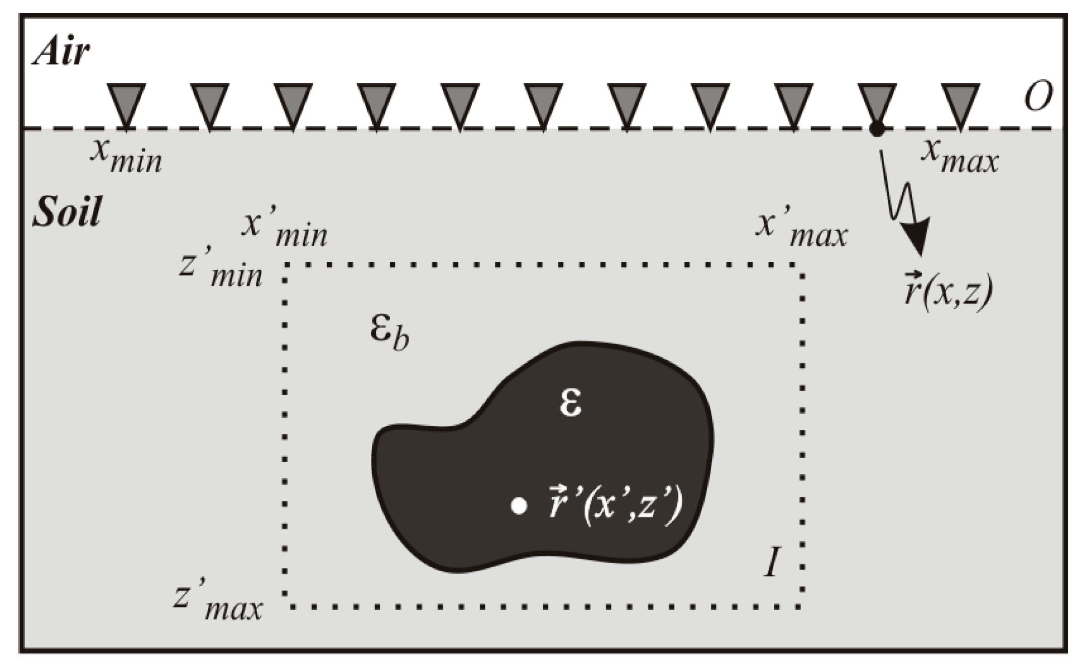
2. Microwave Tomography
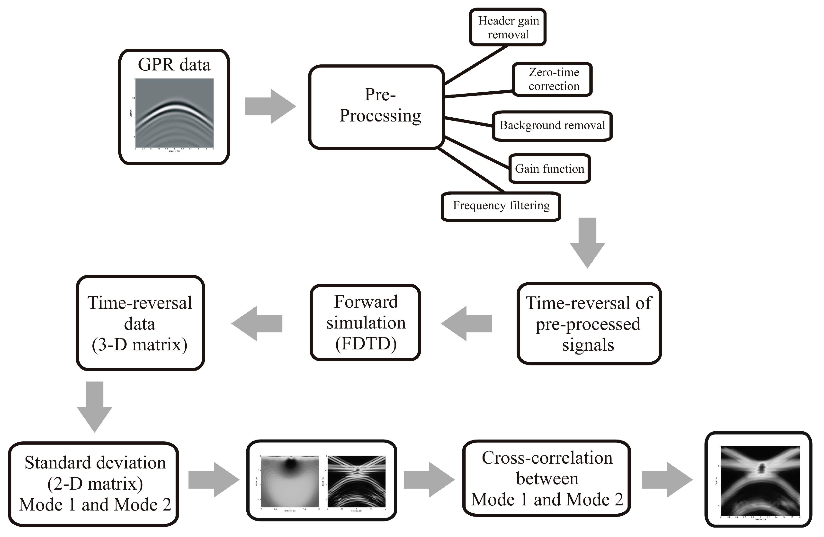
3. Time-Reversal-Based Technique
- (i)
- A short pulse is transmitted from one “or more” transceivers to the region of interest, where it is scattered by one or more targets;
- (ii)
- The scattered signal is registered by the transceivers;
- (iii)
- The received signal waveform is time-reversed (first-in, last-out) and retransmitted (either physically or synthetically) to the region of interest;
- (iv)
- Due to time invariance of the wave equation, the retransmitted waveform will tend to focus around the original target location(s).
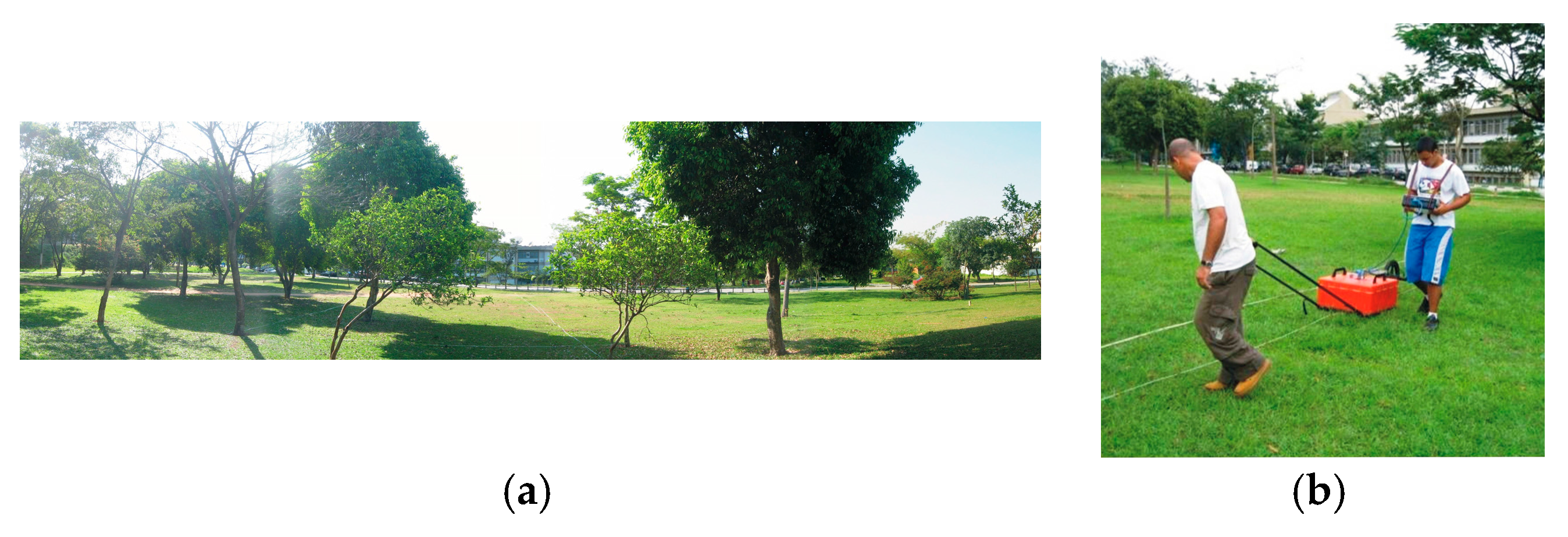
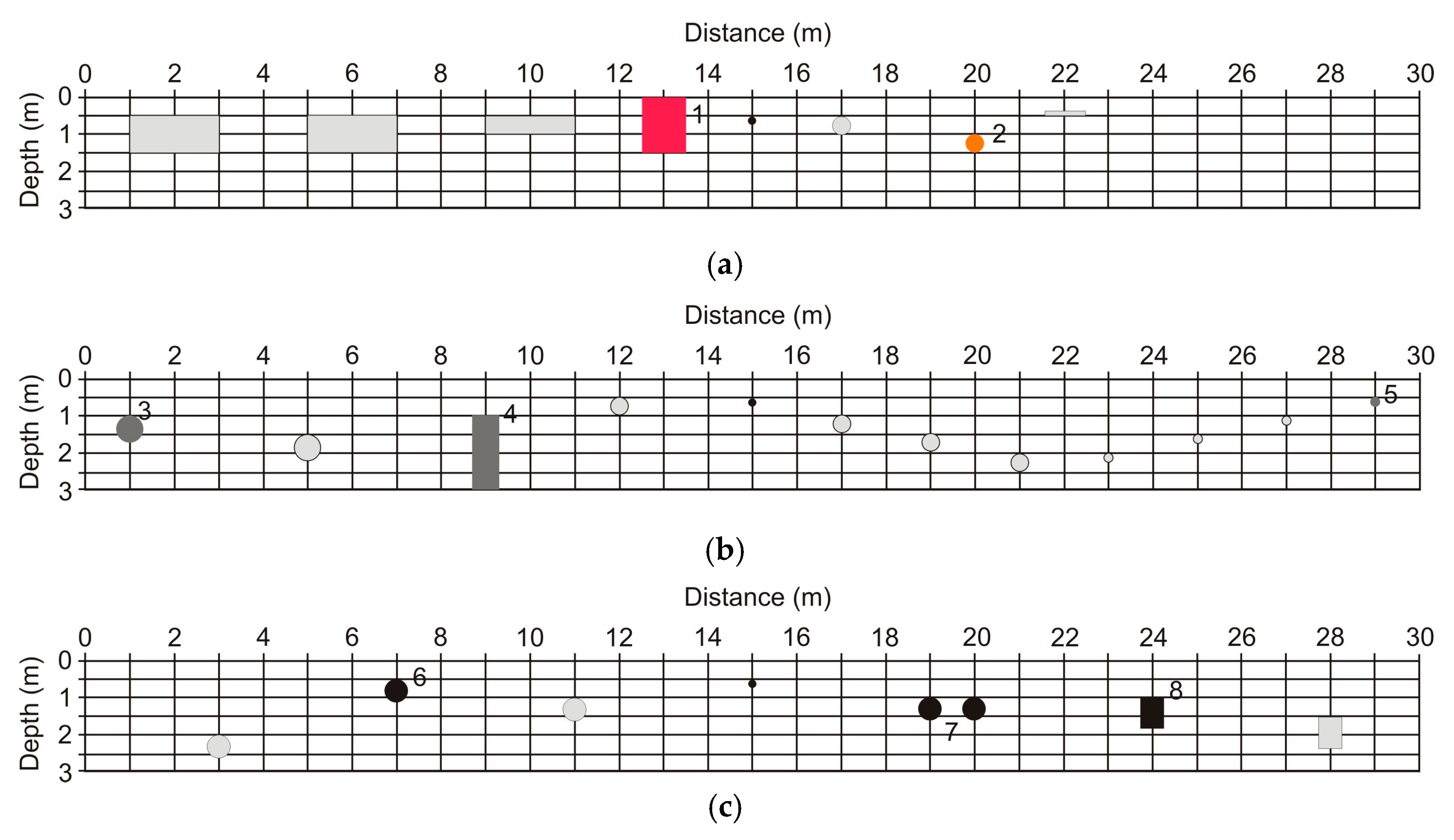
4. Test Site
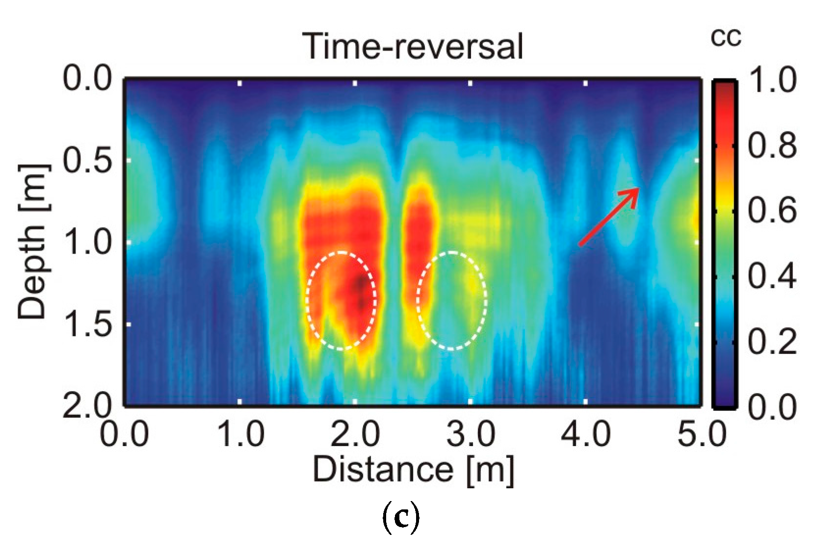
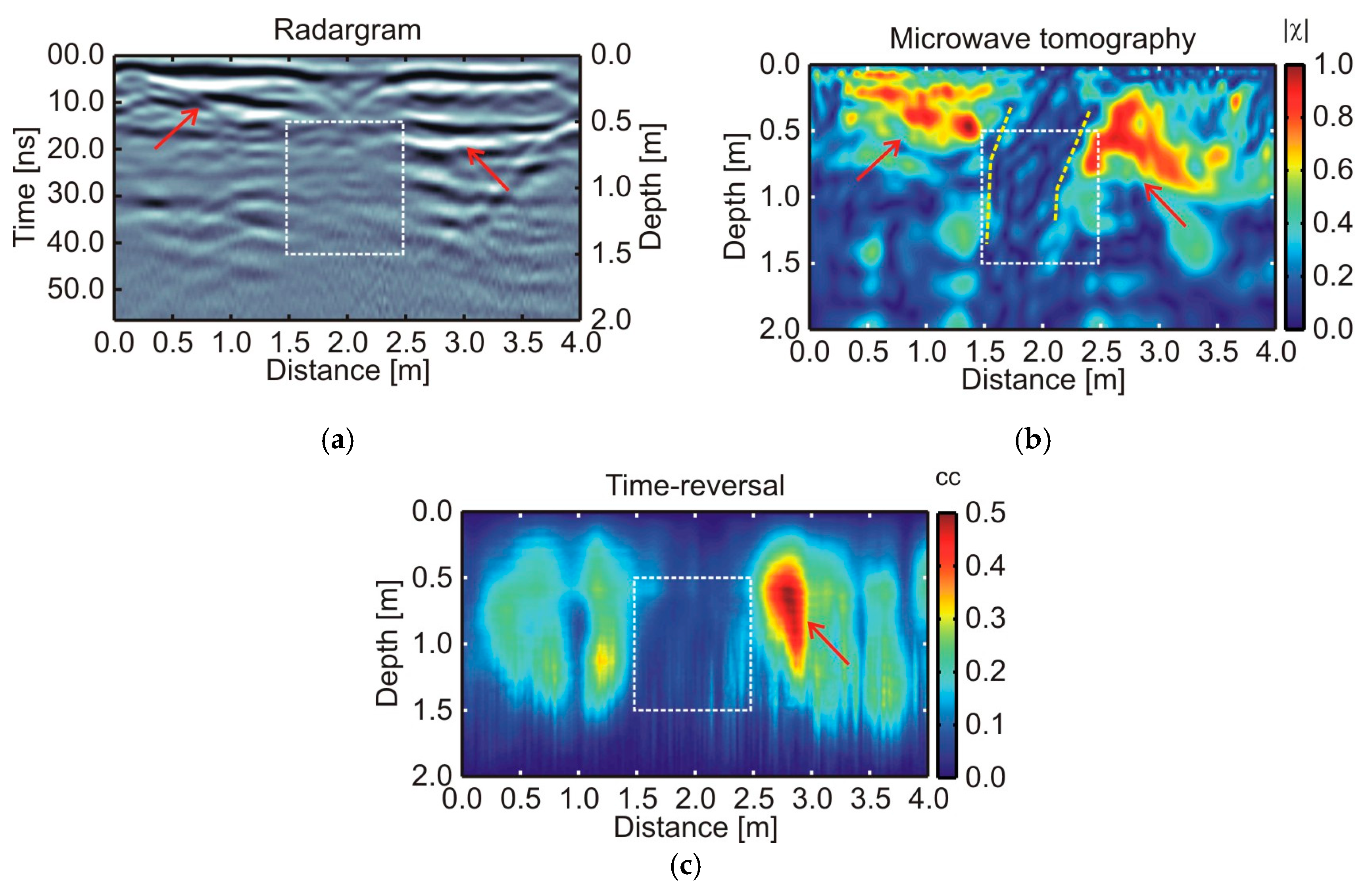
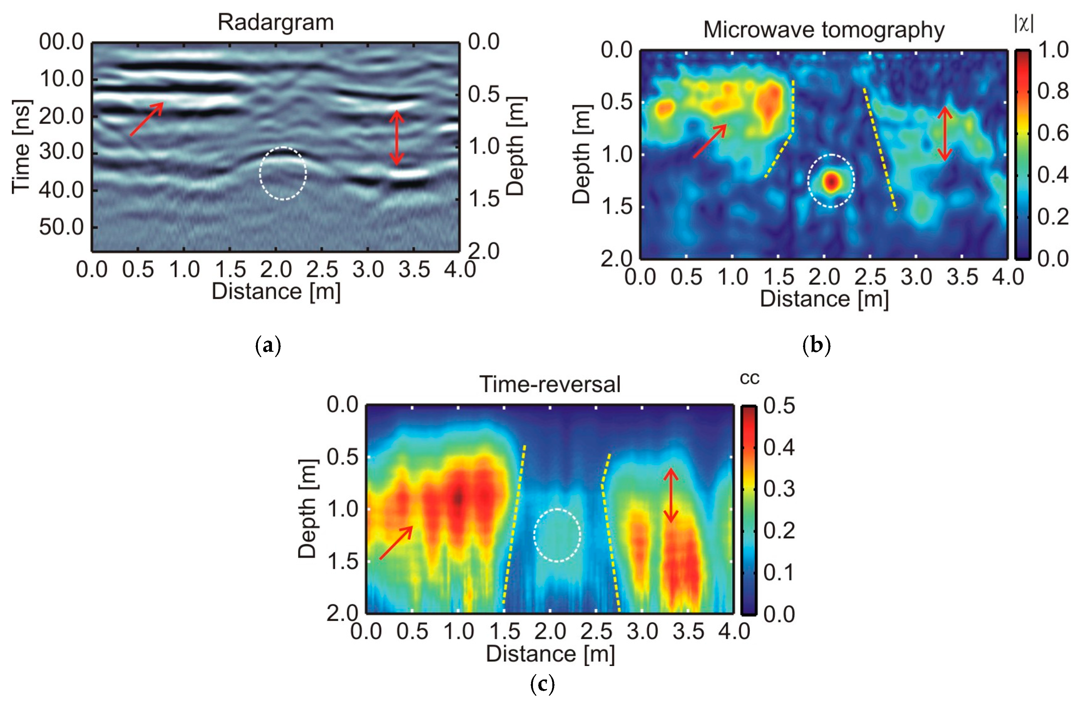
5. Comparative Results
6. Further Discussion
7. Conclusions
Acknowledgments
Author Contributions
Conflicts of Interest
References
- Daniels, D.J. Radar, Sonar, Navigation and Avionics Series 15. In Ground Penetrating Radar, 2nd ed.; IET: Stevenage, UK, 2007; 726p. [Google Scholar]
- Chen, S.Y.; Chew, W.C.; Santos, V.N.; Sainath, K.; Teixeira, F.L. Electromagnetic subsurface remote sensing. In Wiley Encyclopedia of Electrical and Electronics Engineering; Wiley: Hoboken, NJ, USA, 2016. [Google Scholar]
- Shihab, S.; Al-Nuaimy, W. Radius estimation for cylindrical objects detected by ground penetrating radar. Subsurf. Sens. Technol. Appl. 2005, 6, 151–166. [Google Scholar] [CrossRef]
- Alhasanat, M.B.; Hussin, W.M.A. A new algorithm to estimate the size of an underground utility via specific antenna. In Proceedings of the Progress in Electromagnetics Research Symposium (PIERS), Marrakesh, Morocco, 20–23 March 2011; pp. 1868–1870. [Google Scholar]
- Di, Q.; Zhang, M.; Wang, M. Time-domain inversion of GPR data containing attenuation resulting from conductive losses. Geophysics 2006, 71, K103–K109. [Google Scholar] [CrossRef]
- Forte, E.; Dossi, M.; Pipan, M.; Colucci, R.R. Velocity analysis from common offset GPR data inversion: Theory and application to synthetic and real data. Geophys. J. Int. 2014, 197, 1471–1483. [Google Scholar] [CrossRef]
- Babcock, E.; Bradford, J.H. Reflection waveform inversion of ground-penetrating radar data of characterizing thin and ultrathin layers of nonaqueous phase liquid contaminants in stratified media. Geophysics 2015, 80, H1–H11. [Google Scholar] [CrossRef]
- Porsani, J.L.; Sauck, W.A. Ground-penetrating radar profiles over multiple steel tanks: Artifact removal through effective data processing. Geophysics 2007, 72, J77–J83. [Google Scholar] [CrossRef]
- Pettinelli, E.; Di Matteo, A.; Mattei, E.; Crocco, L.; Soldovieri, F.; Redman, J.D.; Annan, A.P. GPR response from buried pipes: Measurement on field site and tomographic reconstructions. IEEE Trans. Geosci. Remote Sens. 2009, 47, 2639–2645. [Google Scholar] [CrossRef]
- Solimene, R.; Cuccaro, A.; Dell’Aversano, A.; Catapano, I.; Soldovieri, F. Ground clutter removal in GPR surveys. IEEE J. Sel. Top. Appl. Earth Obs. Remote Sens. 2014, 7, 792–798. [Google Scholar] [CrossRef]
- Persico, R.; Pochanin, G.; Ruban, V.; Orlenko, A.; Catapano, I.; Soldovieri, F. Performances of a microwave tomographic algorithm for GPR systems working in differential configuration. IEEE J. Sel. Top. Appl. Earth Obs. Remote Sens. 2016, 9, 1343–1356. [Google Scholar] [CrossRef]
- Crocco, L.; Prisco, G.; Soldovieri, F.; Cassidy, N. Early-stage leaking pipes GPR monitoring via microwave tomographic inversion. J. Appl. Geophys. 2009, 67, 270–277. [Google Scholar] [CrossRef]
- Catapano, I.; Affinito, A.; Bertolla, L.; Porsani, J.L.; Soldovieri, F. Oil spill monitoring via microwave tomography enhanced GPR surveys. J. Appl. Geophys. 2014, 108, 95–103. [Google Scholar] [CrossRef]
- Persico, R.; Soldovieri, F. Effects of background removal in linear inverse scattering. IEEE Trans. Geosci. Remote Sens. 2008, 46, 1104–1114. [Google Scholar] [CrossRef]
- Almeida, E.R.; Porsani, J.L.; Catapano, I.; Gennarelli, G.; Soldovieri, F. Microwave tomography-enhanced GPR in forensic surveys: The case study of a tropical environment. IEEE J. Sel. Top. Appl. Earth Obs. Remote Sens. 2016, 9, 115–124. [Google Scholar] [CrossRef]
- Catapano, I.; Soldovieri, F.; Alli, G.; Mollo, G.; Forte, L.A. On the Reconstruction Capabilities of Beamforming and a Microwave Tomographic Approach. IEEE Geosci. Remote Sens. Lett. 2015, 12, 2369–2373. [Google Scholar] [CrossRef]
- Soldovieri, F.; Orlando, L. Novel tomographic based approach and processing strategies for GPR measurements using multifrequency antennas. J. Cult. Heritage 2009, 10, e83–e92. [Google Scholar] [CrossRef]
- Soldovieri, F.; Prisco, G.; Persico, R. A strategy for the determination of the dielectric permittivity of a lossy soil exploiting GPR surface measurements and a cooperative target. J. Appl. Geophys. 2009, 67, 288–295. [Google Scholar] [CrossRef]
- Leucci, G.; Masini, N.; Persico, R.; Soldovieri, F. GPR and sonic tomography for structural restoration: The case of the cathedral of Tricarico. J. Geophys. Eng. 2011, 8, S76–S92. [Google Scholar] [CrossRef]
- Catapano, I.; Crocco, L.; Krellmann, Y.; Triltzsch, G.; Soldovieri, F. A Tomographic Approach for Helicopter-Borne Ground Penetrating Radar Imaging. IEEE Geosci. Remote Sens. Lett. 2012, 9, 378–382. [Google Scholar] [CrossRef]
- Fink, M.A.; Prada, C.; Wu, F.; Cassereau, D. Self-focusing in inhomogeneous media with “time reversal” acoustic mirror. In Proceedings of the Ultrasonics Symposium, Montreal, QC, Canada, 3–6 October 1989; pp. 681–686. [Google Scholar]
- Fink, M.A. Time reversal of ultrasonic field—Part I: Basic principles. IEEE Trans. Ultrason. Ferroelectr. Freq. Control 1992, 39, 555–566. [Google Scholar] [CrossRef] [PubMed]
- Thomas, J.L.; Fink, M.A. Ultrasonic beam focusing through tissue in homogeneities with a time reversal mirror: Application to transskull therapy. IEEE Trans. Ultrason. Ferroelectr. Freq. Control 1996, 43, 1122–1129. [Google Scholar] [CrossRef]
- Tanter, M.; Thomas, J.L.; Fink, M.A. Focusing through skull with time reversal mirrors: Application to hyperthermia. In Proceedings of the IEEE Ultrasonic Symposium, San Antonio, TX, USA, 3–6 November 1996; pp. 1289–1293. [Google Scholar]
- Liu, Z.; Xu, Q.; Gong, Y.; He, C.; Wu, B. A new multichannel time reversal focusing method for circumferential Lamb waves and its applications for detection in thick-wall pipe with large diameter. Ultrasonics 2014, 54, 1967–1976. [Google Scholar] [CrossRef] [PubMed]
- Mora, N.; Rachidi, F.; Rubinstein, M. Application of the time reversal of electromagnetic fields to locate lightning discharges. Atmos. Res. 2012, 117, 78–85. [Google Scholar] [CrossRef]
- Reyes-Rodríguez, S.; Lei, N.; Crowgey, B.; Udpa, L.; Udpa, S.S. Time reversal and microwave techniques for solving inverse problem in non-destructive evaluation. NDT E Int. 2014, 62, 106–114. [Google Scholar] [CrossRef]
- Fink, M.A. Time-reversal acoustics in complex environments. Geophysics 2006, 71, S1151–S1164. [Google Scholar] [CrossRef]
- Artman, B.; Podladtchikov, I.; Witten, B. Source location using time-reverse imaging. Geophys. Prospect. 2010, 58, 861–873. [Google Scholar] [CrossRef]
- Foroozan, F.; Asif, A. Time-reversal ground penetrating radar: Range estimation with Cramér-Rao lower bounds. IEEE Trans. Geosci. Remote Sens. 2010, 48, 3698–3708. [Google Scholar] [CrossRef]
- Yavuz, M.E.; Fouda, A.E.; Teixeira, F.L. GPR signal enhancement using sliding-window space-frequency matrices. Prog. Electromagn. Res. 2014, 145, 1–10. [Google Scholar] [CrossRef]
- Santos, V.R.N.; Teixeira, F.L. Application of time-reversal-based processing techniques to enhance detection of GPR targets. J. Appl. Geophys. 2017, 146, 80–94. [Google Scholar] [CrossRef]
- Santos, V.R.N.; Teixeira, F.L. Study of time-reversal-based signal processing applied to polarimetric GPR detection of elongated targets. J. Appl. Geophys. 2017, 139, 257–268. [Google Scholar] [CrossRef]
- Saillard, M.; Micolau, G.; Tortel, H.; Sabouroux, P.; Geffrin, J.M.; Belkebir, K.; Dubois, A. DORT method and time reversal as applied to subsurface electromagnetic probing. In Proceedings of the 2004 URSI EMTS, International Symposium on Electromagnetic Theory, Pisa, Italy, 23–27 May 2004. [Google Scholar]
- Yavuz, M.E.; Teixeira, F.L. Full time-domain DORT for ultrawideband electromagnetic fields in dispersive, random inhomogeneous media. IEEE Trans. Antennas Propag. 2006, 54, 2305–2315. [Google Scholar] [CrossRef]
- Fouda, A.E.; Teixeira, F.L. Imaging and tracking of targets in clutter using differential time-reversal techniques. Waves Random Complex Media 2012, 22, 66–108. [Google Scholar] [CrossRef]
- Soldovieri, F.; Hugenschmidt, J.; Persico, R.; Leone, G. A linear inverse scattering algorithm for realistic GPR applications. Near Surf. Geophys. 2007, 5, 29–42. [Google Scholar] [CrossRef]
- Leone, G.; Soldovieri, F. Analysis of the distorted Born approximation for subsurface reconstruction: Truncation and uncertainties effects. IEEE Trans. Geosci. Remote Sens. 2003, 41, 66–74. [Google Scholar] [CrossRef]
- Chew, W.C. Electromagnetic Fields in Inhomogeneous Media; IEEE Press: Piscataway, NJ, USA, 1995. [Google Scholar]
- Bertero, M.; Boccacci, P. Introduction to Inverse Problems in Imaging; Institute of Physics: Bristol, UK, 1998. [Google Scholar]
- Harrington, R.F. Field Computation by Moment Methods; Macmillan: New York, NY, USA, 1968; p. 229. [Google Scholar]
- Yavuz, M.E.; Teixeira, F.L. Ultrawideband microwave sensing and imaging using time-reversal techniques: A review. Remote Sens. 2009, 9, 466–495. [Google Scholar] [CrossRef]
- Fink, M.A.; Cassereau, D.; Derode, A.; Prada, C.; Roux, P.; Tamter, M.; Thomas, J.; Wu, F. Time-reversed acoustics. Rep. Prog. Phys. 2000, 63, 1933–1995. [Google Scholar] [CrossRef]
- Papanicolau, G.; Ryzhik, L.; Solna, K. Statistical stability in time reversal. SIAM J. Appl. Math. 2004, 64, 1133–1155. [Google Scholar] [CrossRef]
- Fouda, A.E.; Lopez-Castellanos, V.; Teixeira, F.L. Experimental demonstration of statistical stability in ultrawideband time-reversal imaging. IEEE Geosci. Remote Sens. Lett. 2014, 11, 29–33. [Google Scholar] [CrossRef]
- Fouda, A.E.; Teixeira, F.L. Statistical stability of ultrawideband time-reversal imaging in random media. IEEE Trans. Geosci. Remote Sens. 2014, 52, 870–879. [Google Scholar] [CrossRef]
- Sandmeier, K.J. ReflexW 8.1, Program for the Processing of Seismic, Acoustic or Electromagnetic Reflection, Refraction and Transmission Data; Software Manual: Karlsruhe, Germany, 2016. [Google Scholar]
- Teixeira, F.L.; Chew, W.C.; Straka, M.; Oristaglio, M.L.; Wang, T. Finite-difference time-domain simulation of ground penetrating radar on dispersive, inhomogeneous, and conductive soils. IEEE Trans. Geosci. Remote Sens. 1998, 36, 1928–1937. [Google Scholar] [CrossRef]
- Song, L.P.; Liu, Q.H. Fast three-dimensional electromagnetic nonlinear inversion in layered media with a novel scattering approximation. Inverse Probl. 2004, 20, S171–S194. [Google Scholar] [CrossRef]
- Potter, L.C.; Moses, R.L. Attributed scattering centers for SAR ATR. IEEE Trans. Image Process. 1997, 6, 79–91. [Google Scholar] [CrossRef] [PubMed]
- Trintinalia, L.C.; Bhalla, R.; Ling, H. Scattering center parameterization of wide-angle backscattered data using adaptive Gaussian representation. IEEE Trans. Antennas Propag. 1997, 45, 1664–1668. [Google Scholar] [CrossRef]
- Yavuz, M.E.; Teixeira, F.L. Space–frequency ultrawideband time-reversal imaging. IEEE Trans. Geosci. Remote Sens. 2008, 46, 1115–1124. [Google Scholar] [CrossRef]
- Zhang, T.; Chaumet, P.C.; Mudry, E.; Sentenac, A.; Belkebir, K. Electromagnetic wave imaging of targets buried in a cluttered medium using a hybrid inversion-DORT method. Inverse Probl. 2012, 28. [Google Scholar] [CrossRef]
- Fouda, A.E.; Teixeira, F.L. Bayesian compressive sensing for ultrawideband inverse scattering in random media. Inverse Probl. 2014, 30, 114017. [Google Scholar] [CrossRef]
- Wang, G.L.; Chew, W.C.; Cui, T.J.; Aydiner, A.A.; Wright, D.L.; Smith, D.V. 3D near-to-surface conductivity reconstruction by inversion of VETEM data using the distorted Born iterative method. Inverse Probl. 2004, 20. [Google Scholar] [CrossRef]
- Yu, C.; Yuan, M.; Liu, Q.H. Reconstruction of 3D objects from multi-frequency experimental data with a fast DBIM-BCGS method. Inverse Probl. 2009, 25, 024007. [Google Scholar] [CrossRef]


| Targets | Description | |
|---|---|---|
| 1 | Disturbed soil | Disturbed soil, with 1 m3 volume |
| 2 | Ceramic vase | Empty ceramic vase, with 0.55 m diameter and 1.0 m depth |
| 3 | Concrete tube | Horizontal concrete tube (with iron structure), with 0.7 m diam. and 1.0 m depth |
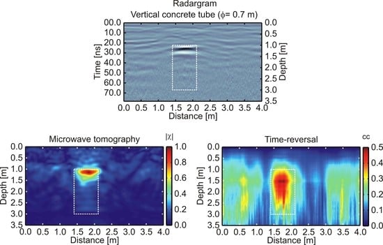
| 4 | Concrete tube | Vertical concrete tube (with iron structure), with 0.7 m diam. and 1.0 m depth |
| 5 | Concrete tube | Horizontal concrete tube, with 0.26 m diameter and 0.5 m depth |
| 6 | Metallic tank | Horizontal metallic tank with 0.59 m diameter and 0.5 m depth |
| 7 | Metallic tank | Double horizontal metallic tanks with 0.59 m diameter and 1.0 m depth |
| 8 | Metallic tank | Vertical metallic tank with 0.86 m height and 1.0 m depth |
| Target | [S/m] | Size (m) | |
|---|---|---|---|
| disturbed soil | 18.0 | 0.007 | 2.85λ18 |
| ceramic vase | 18.0 | 0.007 | 1.57λ18 (φ) |
| horizontal concrete tube | 11.1 | 0.001 | 1.55λ11 (φ) |
| vertical concrete tube | 11.1 | 0.001 | 1.55λ11 (φ) 2.22λ11 (h) |
| horizontal concrete tube | 11.1 | 0.001 | 0.57λ11 (φ) |
| horizontal metallic storage tank | 18.0 | 0.007 | 1.68λ18 (φ) |
| pair of horizontal metallic storage tanks | 18.0 | 0.007 | 1.68λ18 (φ) 2.86λ18 (s) |
| vertical metallic storage tank | 18.0 | 0.007 | 1.68λ18 (φ) 2.46λ18 (h) |
| Target | TSVD Threshold Value [dB] | TSVD Threshold Index |
|---|---|---|
| disturbed soil | −27.5 | 728 |
| ceramic vase | −30.7 | 782 |
| horizontal concrete tube | −25.6 | 630 |
| vertical concrete tube | −25.1 | 626 |
| horizontal concrete tube | −16.3 | 169 |
| horizontal metallic storage tank | −31.5 | 1010 |
| pair of horizontal metallic storage tanks | −42.3 | 1150 |
| vertical metallic storage tank | −24.8 | 643 |
© 2018 by the authors. Licensee MDPI, Basel, Switzerland. This article is an open access article distributed under the terms and conditions of the Creative Commons Attribution (CC BY) license (http://creativecommons.org/licenses/by/4.0/).
Share and Cite
Dos Santos, V.R.N.; Almeida, E.R.; Porsani, J.L.; Teixeira, F.L.; Soldovieri, F. A Controlled-Site Comparison of Microwave Tomography and Time-Reversal Imaging Techniques for GPR Surveys. Remote Sens. 2018, 10, 214. https://doi.org/10.3390/rs10020214
Dos Santos VRN, Almeida ER, Porsani JL, Teixeira FL, Soldovieri F. A Controlled-Site Comparison of Microwave Tomography and Time-Reversal Imaging Techniques for GPR Surveys. Remote Sensing. 2018; 10(2):214. https://doi.org/10.3390/rs10020214
Chicago/Turabian StyleDos Santos, Vinicius Rafael Neris, Emerson Rodrigo Almeida, Jorge Luís Porsani, Fernando Lisboa Teixeira, and Francesco Soldovieri. 2018. "A Controlled-Site Comparison of Microwave Tomography and Time-Reversal Imaging Techniques for GPR Surveys" Remote Sensing 10, no. 2: 214. https://doi.org/10.3390/rs10020214
APA StyleDos Santos, V. R. N., Almeida, E. R., Porsani, J. L., Teixeira, F. L., & Soldovieri, F. (2018). A Controlled-Site Comparison of Microwave Tomography and Time-Reversal Imaging Techniques for GPR Surveys. Remote Sensing, 10(2), 214. https://doi.org/10.3390/rs10020214