1. Introduction
Forests play a key role in the terrestrial ecosystem and have a large amount of economic, ecological, and social benefits because they regulate the water cycle and carbon cycle on the surface of the Earth [
1]. For effective forest management and human activity documentation, the forest inventory for sustainable forest management is usually needed to obtain a great number of single tree-related parameters, such as tree species and tree species distribution, timber volume, increment of timber volume, and mean tree height [
2,
3,
4,
5,
6,
7,
8,
9]. Traditionally, in practice, most single-tree-level parameters are estimated by manually sampling small plots in a field survey, which is time consuming and labor intensive [
10,
11].
In recent years, airborne light detection and ranging (LiDAR) has become an emerging remote sensing technique for performing forest inventory tasks because it can penetrate through tree canopies and acquire three-dimensional (3D) forest structures [
12,
13]. LiDAR technology can improve the accuracy of forest parameter retrieval at the single-tree level because of its capability of providing accurate and spatially detailed information of tree structure elements (such as branches and foliage) [
14]. Currently, airborne LiDAR is considered to be a standard data source for deriving forest spectral and spatial information at the scale of single trees because it provides timely, large-scale, and accurate forest information to support forest management. Matasci et al. [
2] demonstrated that the integration of airborne LiDAR and Landsat-derived reflectance products predicted a total of 10 forest structural attributes by using a nearest neighbor imputation approach based on the random forest framework, with
R2 values ranging from 0.49–0.61 for key response variables such as canopy cover, stand height, basal area, and stem volume. Allouis et al. [
3] estimated stem volume and aboveground biomass from the single-tree metrics derived from full-waveform LiDAR data by using regression models and improved the accuracy of aboveground biomass estimates. Matsuki et al. [
4] obtained a tree species classification accuracy of 82% by integrating spectral features obtained from hyperspectral data and tree-crown features derived from LiDAR data with a support vector machine classifier. However, it is still difficult to detect single trees automatically from airborne LiDAR data due to the various shapes of trees and their periodic changes with the seasons, especially to segment trees with complex and heterogeneous crowns.
With the development of unmanned aerial vehicles (UAV) technologies in weight capacity, durability, and controlling, UAV LiDAR systems have been proposed to be an alternative means for capturing 3D canopy structural information. Compared to airborne LiDAR, UAV LiDAR has been shown to be lower cost, which can monitor key development stages of forest management in a timely manner, such as pruning, thinning, and harvesting [
15]. Moreover, it is more flexible and controllable in terms of flying altitude, viewing angles, and forward and side overlap with fine spatial and temporal resolutions [
16]. Furthermore, UAV LiDAR can avoid some complications, such as plane flight logistics, cloud covers, and atmospheric effects [
17]. Because UAV and airborne LiDAR data show certain similar characteristics, most researchers segmented single trees from UAV LiDAR data by using the algorithms that are usually applied to airborne LiDAR data.
Many methods have been proposed for detecting and delineating single trees from airborne LiDAR points. These methods can be generally categorized into two categories, i.e., raster-based and point-based methods, in terms of data types used [
18]. Raster-based methods first interpolate point clouds into a two-dimensional (2D) canopy height model (CHM), in which potential stem positions are located based on the local maxima, and then, tree crowns are delineated by using the established image processing algorithms, such as watershed segmentation, valley following, template matching, and region growing [
19,
20,
21]. However, raster-based methods heavily rely on the accuracy of the constructed CHM. Moreover, these methods usually fail to detect and delineate some smaller trees under the canopies and closely neighboring trees especially in dense and heterogeneous forests [
22]. Consequently, some improvements have been proposed. For example, a filtering CHM and variable window strategy have been presented to reduce the misclassification of local maxima caused by the noise in CHM [
20,
21]. Wallace et al. [
15] demonstrated that high density UAV LiDAR points contributed to the improvement of the tree extraction accuracy. Hyyppä et al. [
1] detected trees by using the last pulse data, which improved the tree detection accuracy by 6%. However, these raster-based methods use only tree elevation information of the constructed CHM, and 3D spatial information of LiDAR data has been ignored [
23].
To make full use of the 3D structures of point clouds, in recent years, many researchers have identified single trees directly from original LiDAR data [
23,
24,
25]. Morsdorf et al. [
26] segmented trees in a 3D voxel space with a
k-means clustering method by using the local maxima of the CHM as seed points. Gupta et al. [
27] improved Morsdorf’s method by scaling down height values to increase the similarity between point clouds. However, these methods also relied on the local maxima detected in CHM data. Region growing has been widely used in single-tree delineation from airborne LiDAR data. Lee et al. [
21] first defined an optimal moving window size to detect all possible seed points with an overall accuracy of 95.1%. However, it required ground truth data as training data to achieve the optimal results. Li et al. [
22] proposed a top-to-down region-growing algorithm based on the relative tree spacing to detect single trees. The method performed well in conifer forest, but it worked less effectively when applied to a deciduous forest. Lu et al. [
25] segmented single trees with an overall
F-score of 0.9. However, the method required intensity information and could be only applied to leaf-off conditions, which limited the further applications. These clustering methods are unsuitable to deal with forests with overlapped canopies because they can hardly find appropriate parameters for large-scale forest environments or staggered stems in deciduous forests. Moreover, the above single-tree segmentation methods have certain restrictions on tree species and LiDAR data, and their segmentation accuracies on overlapped canopies are usually unsatisfactory.
Ferraz et al. [
28] presented an improved mean shift algorithm, considering both density and height factors to detect tree apices in multi-layered forests. Dai et al. [
29] improved the tree detection accuracy by using multispectral airborne LiDAR. A mean shift method is capable of locating tree apices according to the density and height maxima of point clouds without prior knowledge of the number of clusters or depending on the interpolated 2D CHM data. To delineate small trees under canopies from airborne LiDAR data, Reitberger et al. [
30] introduced normalized cut (NCut), originally proposed for 2D image segmentation, and achieved a recognition rate of 12%, which is higher than conventional watershed segmentation methods. Zhong et al. [
31] improved the algorithm to segment overlapped trees with a correctness of above 90% by means of terrestrial and mobile LiDAR data. NCut has shown great potential in 3D segmentation and works very well when separating two overlapping objects [
32,
33]. However, the traditional NCut has difficulty in accurately locating tree stems in airborne/UAV LiDAR data due to the lack of understory information in severely-overlapped forests.
The objective of this study aims to propose an automated hierarchical single-tree delineation approach, as well as applying and assessing the feasibility of the proposed algorithm using high-density UAV LiDAR data. The remainder of the paper is organized as follows:
Section 2 describes the study area and UAV LiDAR data acquired from a Velodyne 16E system.
Section 3 details the proposed single-tree segmentation method using UAV LiDAR data. The method starts with the normalization and segmentation of non-ground points from the Velodyne 16E UAV LiDAR data. After that, to improve data processing efficiency, a voxel-based mean shift algorithm is used to roughly obtain well-detected and under-segmentation clusters. Finally, to delineate overlapped trees effectively, an improved normalized cut (NCut) segmentation method is proposed to segment under-segmentation clusters iteratively into single trees with a tree apex detection strategy. The conducted tests are described and analyzed in
Section 4. Finally, concluding remarks are given in
Section 5.
2. Test UAV LiDAR Data
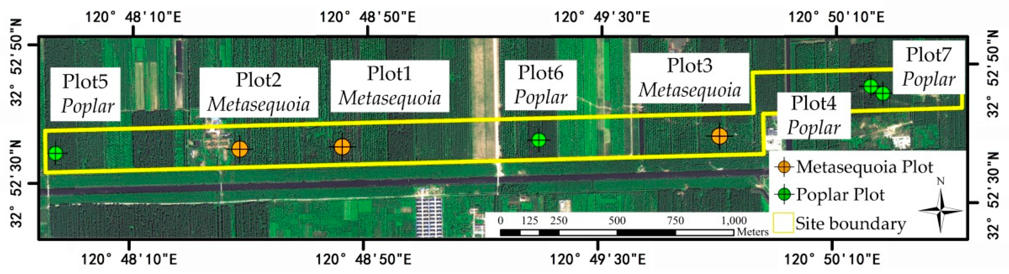
The study area (marked by a large yellow frame in
Figure 1) is about 54.67 hectares and located in Dongtai forest farm with relatively flat terrain, Yancheng City, Jiangsu, China. The specific location of the study area is detailed in
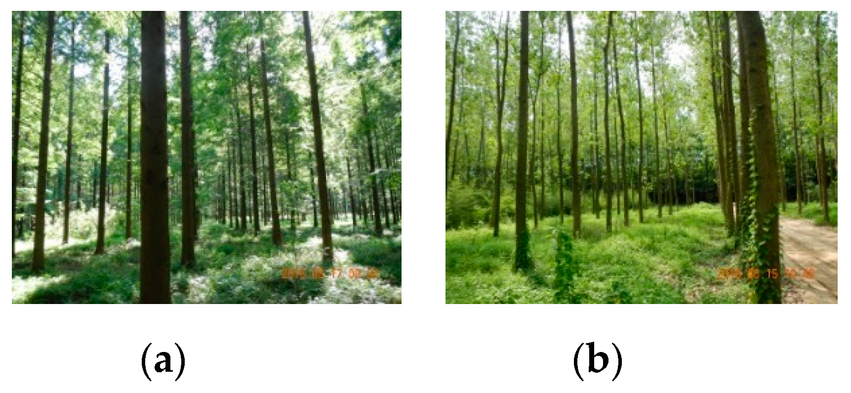
Figure 1. The trees in the forest farm were planted in almost the same period of time, leading to approximate similarities of these trees in shape and size. The test site dominantly covers two tree species:
Metasequoia and
Poplar.
Metasequoia, a fast-growing, deciduous tree, and the sole living species, has a cone-shaped canopy with sparse branches and leaves, as shown in
Figure 2a.
Poplar, a genus of 25–35 species of deciduous flowering plants, is among the most important boreal broadleaf trees in northern cities of China.
Poplar has an irregular shape (see
Figure 2b) with spirally-arranged leaves that vary in shape from triangular to circular or lobed, and with a long petiole.
The research data were collected by a laser scanner system mounted on a GV1300 multi-rotor UAV produced by Green Valley International. The serial number of the UAV LiDAR system is LA2016-003. The UAV platform is composed of the following components: eight brushless motors, a Novatel initial measurement unit (IMU-IGM-S1), a dual-frequency GPS (global positioning system) produced by Novatel, and a ground control system to track the aircraft, control the UAV-LiDAR system, and continuously monitor UAV flying parameters. The main components of the UAV platform can be seen in
Figure 3. Lin et al. [
34] demonstrated the advantages of these sensors integrated on a UAV platform and the feasibility of the UAV development. Besides, a Novatel global navigation satellite system ground base station was used to ensure GPS accuracies. The real-time UAV LiDAR data were transferred to the ground data terminals through a long-range Wi-Fi system connected to the UAV [
35]. The parameters of the UAV platform are listed in
Table 1.
The UAV LiDAR data were acquired with a point density of 40.57 points/m
2 on 24–26 July 2017, by a VLP16 (Velodyne 16E) laser scanner system produced by Velodyne LiDAR. The full specifications of VLP16 are listed in
Table 2. Note that, in this study, the LiDAR data accuracy, which usually requires being evaluated based on the ground control points measured by a total station and creating a reference dataset [
36,
37], was unavailable; therefore, the data accuracy was directly reflected by the system’s ranging accuracy.
To evaluate the single-tree segmentation accuracy, the reference data were collected in July 2017, by field measurements and a backpack laser scanning system produced by Green Valley International. The full specifications of the backpack laser scanning system are listed in
Table 3. According to the producer, the data accuracy was about 5 cm. Seven reference plots were selected to evaluate the single-tree segmentation accuracy in the study site, as shown in
Figure 1, including three samples of
Metasequoia (Plots 1, 2, and 3) and four samples of
Poplar (Plots 4, 5, 6, and 7). Each tree within the plots was located by the backpack laser scanning system. Each plot was 30 m × 30 m in size. The numbers of the reference trees for Plots 1–7 were 29, 54, 54, 18, 20, 21, and 42, respectively. Accordingly, their forest densities were 0.032, 0.060, 0.060, 0.020, 0.022, 0.023, and 0.047 trees/m
2, respectively. Within each plot, the location and the diameter at breast height (DBH) of each tree were recorded.
3. Methodology
To obtain single trees segmented from UAV LiDAR data, our proposed approach includes the following steps: (1) data preprocessing, which first separates ground points from non-ground points and normalizes the UAV LiDAR data according to the produced DTM from the filtered ground points, (2) a voxel-based mean shift method, which voxelizes and roughly segments non-ground points into well-detected and under-segmentation clusters, and (3) an improved normalized cut segmentation method, based on a tree apex detection strategy, which iteratively identifies single trees from the under-segmentation clusters that contain multiple overlapped trees.
3.1. Data Pre-processing
In the data preprocessing procedure, to reduce computational complexity, a ground filtering method based on cloth simulation (CSF), developed by Zhang et al. [
38], was utilized to classify UAV LiDAR points into ground and non-ground points because it needs a few parameters that are easy to set and adapts to various terrains without tedious parameter setting. The CSF algorithm first turns the terrain upside down and places a cloth on the inverted surface from above, then determines the final shape of the cloth to separate ground from non-ground points by analyzing the interaction between the nodes of the cloth and the corresponding LiDAR points. The CSF algorithm consists of four user-defined parameters: rigidness (
FRI), steep slope fit factor (
FST), grid resolution (
FGR), and time step (
FDT). The first two parameters are the key parameters, which control the filtering results, and vary with terrain types. The last two parameters are usually fix-valued and universally applicable to all LiDAR datasets. The detailed description of the CSF algorithm can be found in [
38]. The ground points were then interpolated into a digital terrain model (DTM) by linear interpolation. Afterward, to reduce the influence of undulating terrain on single-tree recognition and tree height extraction, the non-ground points were normalized according to the produced DTM with a spatial resolution of 0.5 m. Moreover, low-rise shrubs in the forests were removed by a given height threshold (
Γh).
3.2. Voxel-Based Mean Shift
The point cloud data, acquired by a UAV LiDAR system, contained a considerable number of points; however, point-wise processing methods are usually time consuming and computationally complex. To reduce data redundancy and improve data processing efficiency, a voxelization strategy was introduced in this study. The non-ground points were segmented into a number of voxels with a given voxel size (Vs). The voxel size depends on the point density of the UAV LiDAR points to be processed. We statistically counted the number of points and determined the center of all the points for each voxel. The voxelization for UAV LiDAR points contributes to improving the computational efficiency and maintaining feature details of objects, which has been widely used for point cloud registration, surface reconstruction, shape recognition, etc.
After voxelization, mean shift, proposed by Ferraz et al. [
28], was used to segment single trees roughly with the local maxima based on the density function. All non-ground UAV LiDAR points in the form of voxels can be regarded as a multimodal distribution, where each mode, here defined as a local maximum in both density and height, corresponds to a crown apex [
28].
The algorithm starts with selecting the highest voxel,
Xc = (
xc,
yc,
zc), in the non-ground voxels and obtaining all its neighboring voxels,
Xi = (
xi,
yi,
zi) (
i = 1, 2, 3, …,
n), where
n is the number of voxels within a given radius,
R. Next, we calculated the offset vector by summing the vectors between the voxel and its neighboring voxels. To converge voxels within each crown toward the corresponding crown apex, a 3D space was separated into horizontal and vertical directions. The horizontal kernel was defined for searching local density maxima, and the vertical one for local height maxima [
29]. Therefore, the offset vector of voxel
Xi to voxel
Xc is defined by:
where the superscripts
s and
r refer to the horizontal and vertical directions, respectively.
xcs and
xcr are the horizontal and vertical vector components of voxel
Xc, respectively.
xis and
xir are the horizontal and vertical vector components of voxel
Xi, respectively. The horizontal and vertical bandwidths (
hs,
hr) represent the width and depth of a canopy.
gs is the horizontal kernel function that follows a Gaussian function:
The vertical kernel,
gr, is specially-designed for assigning a larger weight to the highest voxel:
where
mask(
xcr,
xir) represents a mask of foreground object;
dist(
xcr,
xir) is the distance between
Xi and the boundary of the mask. They are defined by,
Then, voxel Xc moves along the offset vector until it reaches the density and height maxima and labels all voxels visited during this process as the same cluster. The proposed voxel-based mean shift method repeats the above steps until all voxels in the non-ground points are visited and labeled into specific clusters. Afterward, the nearby clusters, whose distances are less than a given distance threshold, Γd, are merged together. In the study, to increase the similarity of all voxels belonging to a single tree, the proposed method compresses (m, a multiple of height compression) the point height to improve the clustering results.
With the voxel-based mean shift method, the non-ground voxels were roughly segmented into a set of local clusters. For each cluster, we projected all voxels onto the XOY plane and calculated the diameters in the x- and y-directions (d1 and d2). According to the ratio of d1 to d2, the clusters will be classified into two groups: well-detected and under-segmentation clusters. Here, we defined that a well-detected cluster is a single tree with circular-shaped canopy, while an under-segmentation cluster is an irregularly-shaped one containing more than two trees. Thus, if the ratio of d1 to d2 was close to 1, the cluster was labeled as well-detected (i.e., a single tree), otherwise the cluster was labeled as under-segmentation.
3.3. Improved Normalized Cut Single-Tree Segmentation
To delineate single trees from the under-segmentation clusters that contain multiple overlapped trees and objects, an improved NCut segmentation algorithm was introduced.
3.3.1. Normalized Cut
NCut aims to solve the graph partitioning problem in 2D image segmentation [
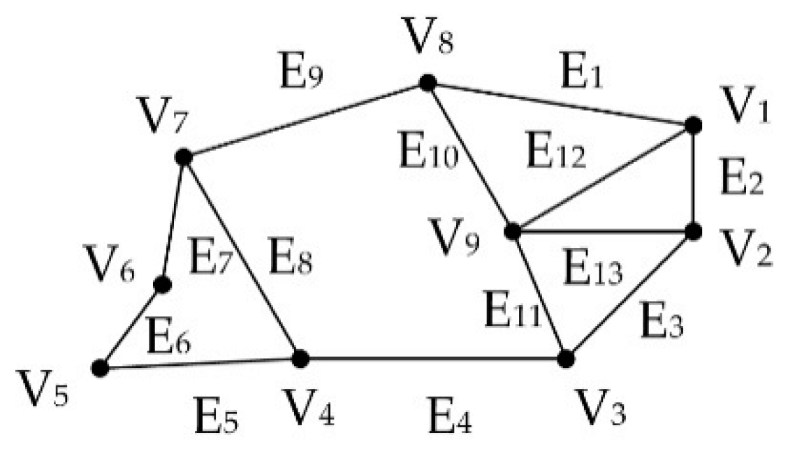
39]. It works on a weighted connected graph. The idea behind the algorithm is that, by using dynamic programming, a given object is segmented by minimizing the cost for cutting the weighted connected graph into two sub-graphs. The algorithm has been extended to 3D space. The non-empty voxels were used to construct a weighted graph
G = {
V,
E} (see
Figure 4), where
V is a set of graph nodes representing the voxels and
E is the set of graph edges that connect the nodes.
Denote weight
wij as the similarity between a pair of nodes {
i,
j} ϵ
V. It is computed as follows:
where
DijXY,
DijZ, and
DijS represent the horizontal, vertical, and shortest distances, respectively, between nodes
i and
j.
σXY,
σZ, and
σS are coefficients, set to be 0.05-times the maximum of
DijXY,
DijZ, and
DijS, for controlling the sensitivity of the impact factors, respectively.
ΓR represents the maximum horizontal distance threshold between nodes.
wij = 0, if the horizontal distance between nodes {
i,j} exceed the threshold,
ΓR. NCut aims to divide the graph
G into two disjoint voxel groups
A and
B by maximizing the similarity within each voxel group and minimizing the similarity between two voxel groups
A and
B. The corresponding cost function is as follows:
where
is the sum of weights between voxel groups
A and
B.
and
represent the sums of weights of all edges ending in the voxel groups
A and
B, respectively. To segment voxel groups
A and
B exactly,
is minimized and solved by the corresponding generalized eigenvalue equation:
where
W is an
n ×
n weighting matrix representing the weights between all nodes of graph
G.
D is an
n × n diagonal matrix, and
.
λ is an eigenvalue, and
y represents the eigenvector corresponding to the generalized eigenvalue. The minimum solution,
y1, to Equation (8) corresponds to the second smallest eigenvalue,
λ1 [
23].
3.3.2. Improved NCut
The traditional NCut algorithm has difficulty in accurately locating tree stems in airborne/UAV LiDAR data due to the lack of understory information in severely-overlapped forests. NCut requires the specific number of single trees in point cloud data to be processed. Therefore, in the study, to segment single trees from the under-segmentation clusters containing multiple overlapped objects, we improved the NCut algorithm by adopting a tree apex detection strategy, which is capable of automatically determining the number of single trees in the clusters. The tree apex detection strategy starts with profile generation, which sections the cluster into a set of profiles both in the x- and y-direction with a user-defined profile size,
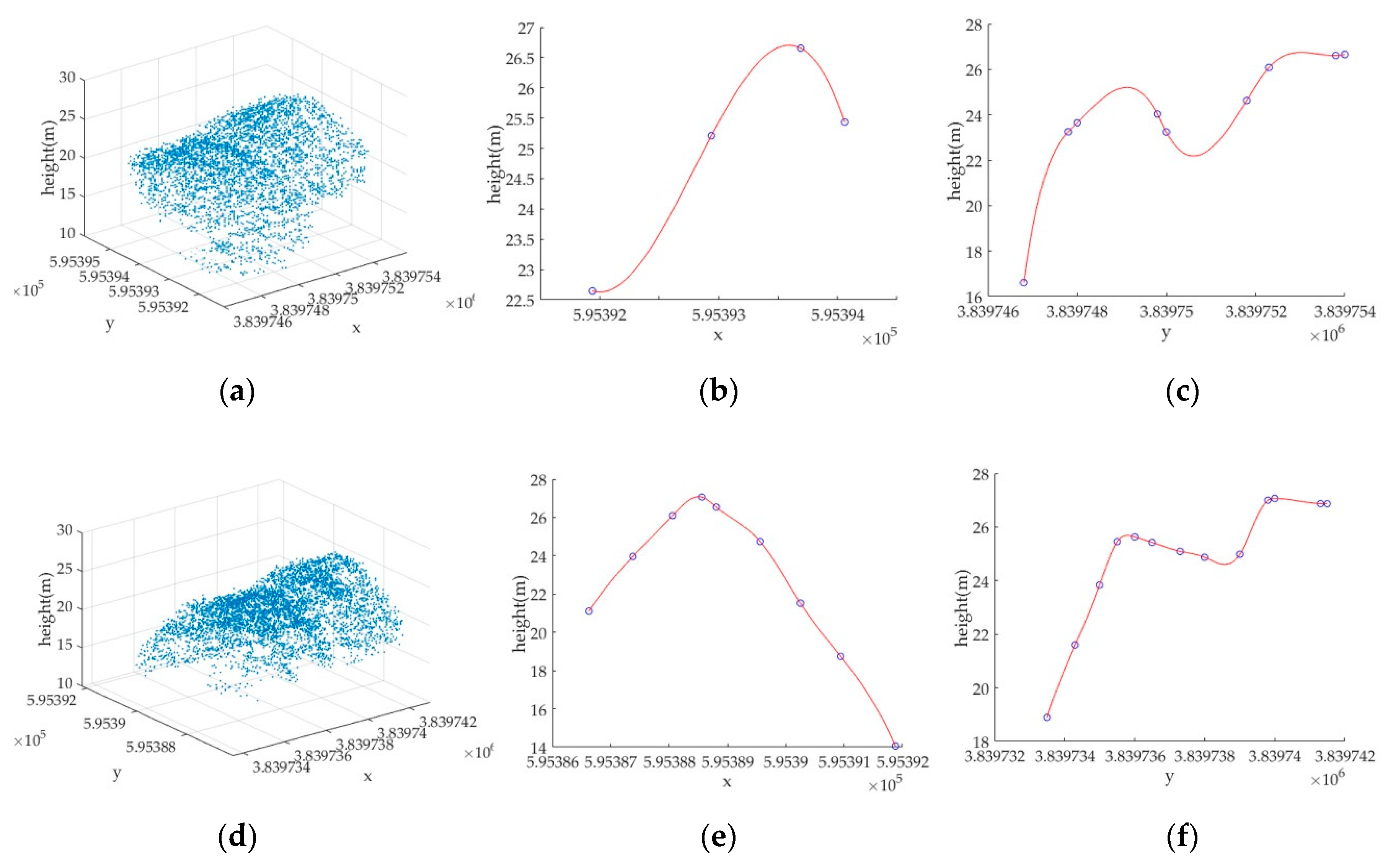
Γs. The profiles generated both in the x- and y-direction help reduce the occlusions. For each profile in the x- and y-direction, respectively, we calculate the maximum height for generating shape curves by cubic spline data interpolation.
Figure 5 shows two clusters and their corresponding shape curves.
Figure 5a,d show two clusters in the form of 3D points,
Figure 5b,e their corresponding shape curves in the x–direction and
Figure 5c,f the shape curves in the y-direction. The peaks of the generated shape curves both in the x- and y-direction are found to determine tree apices, which means the number of peaks in the shape curves determines the number of potential single trees to be segmented in the under-segmentation cluster.
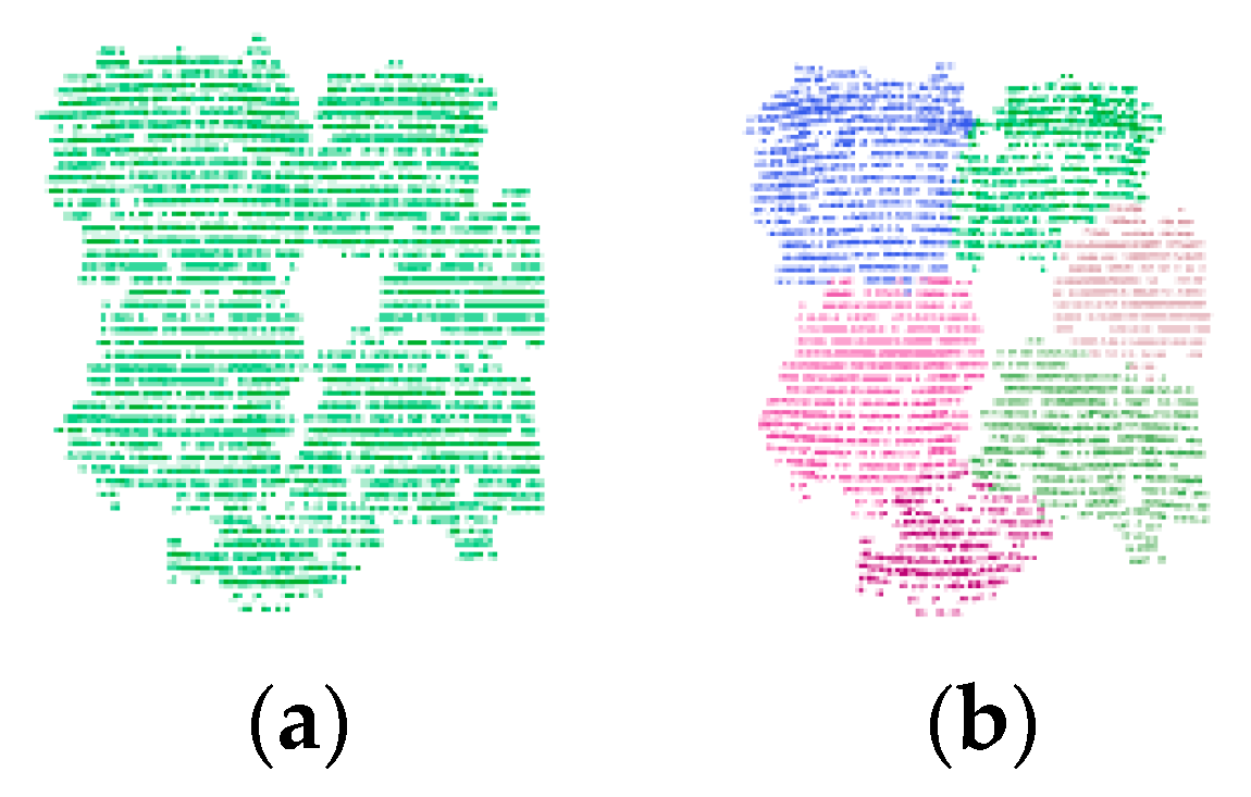
With the determined number of potential tree apices, the NCut iteratively segments the cluster into the specified number of single trees.
Figure 6a shows an example of an under-segmentation cluster with multiple overlapped trees. As seen in
Figure 6b, the cluster is further segmented into six potential single trees.
4. Experimental Results and Discussion
The proposed single-tree segmentation method was performed using Microsoft Visual Studio 2013 (programed using C++) and MATLAB 2016a and tested on an HP Z820 eight-core-16-thread workstation. To evaluate the proposed single-tree segmentation method qualitatively and quantitatively, we conducted a set of experiments on seven reference plots. In this study, we segmented single trees based on tree apices, which might lead to an identification error between the location of the segmented single tree and the reference data. If the identification error was within a certain range or the majority of points (over 80%) belonging to the segmented single tree were correctly identified, we considered that the single tree was correctly identified.
Before we investigated the applicability and feasibility of the proposed single-tree segmentation method, several parameters were empirically selected in advance, according to prior acknowledge of the UAV LiDAR data and the test site. As seen in
Table 4, in the data preprocessing, five parameters—
FRI,
FST,
FGR,
FDT, and
Γh—were used.
FRI represented the terrain type and was set to three according to the flat terrain.
FST decided whether the post-processing of steep slopes was required.
FGR and
FDT were respectively set to 0.5 and 0.65, which were adapted to most of the scenes.
FGR represented the horizontal distance between two neighboring points, and
FDT controlled the displacement of points from gravity during each iteration. Low-rise shrub height threshold,
Γh, was set to 5.0 m according to the tree height in the test site. In the voxel-based mean shift algorithm, six parameters—
Vs,
m, R,
Γd,
hs, and
hr—were used to obtain a set of clusters. The voxel size,
Vs, was set according to the point density. To increase the similarity in vertical distance,
m was set to four. The search radius,
R, and the minimum distance between clusters,
Γd, were both set to 2.0 m according to the average width of canopies in the study
. hs and
hr were two bandwidths of the horizontal and vertical kernels, which represented the range where the local density and local maxima existed.
hs and
hr were set to 1.5 m and 5.0 m, respectively, according to the average width and depth of the tree canopies in the test site. In the improved NCut-based single-tree segmentation stage,
Γs, the profile size in the x- and y-direction was set to 0.5 m based on the defined voxel size. The maximum horizontal distance threshold between the cluster nodes,
ΓR, was empirically set to 4.5 m according to the average width of tree canopies.
The accuracy of the proposed method was evaluated by the following three measurements: correctness (
Ecor), completeness (
Ecpt), and
F-score (
Ef).
Ecor indicates what percentage of the segmented single trees were valid, whereas
Ecpt describes how complete the detected single trees were.
Ecor is defined as
Ecor =
Cp/
Ep, and
Ecpt is expressed as
Ecpt =
Cp/
Rf, where
Cp denotes the number of real single trees,
Rf is the number of single trees in the reference data, and
Ep represents the number of single trees segmented by our method.
Ef evaluates the overall accuracy, which is defined as:
4.1. Overall Performance
To evaluate the performance of our proposed single-tree segmentation method, we applied it to the UAV LiDAR data set. Two tree species,
Metasequoia and
Poplar, were tested. The parameters involved in this study were set according to
Table 4. The UAV LiDAR data in the test site were first preprocessed to obtain the normalized non-ground points. The ground points were compared with the reference DTM, which was manually processed by means of a Terrasolid© software (
http://www.terrasolid.com/home.php). The root mean squared error (RMSE) was 0.23 m, referring to the evaluation method in [
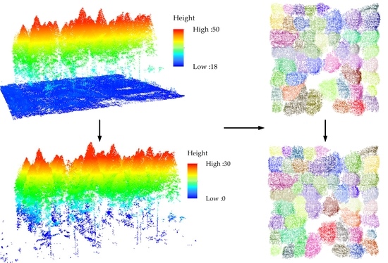
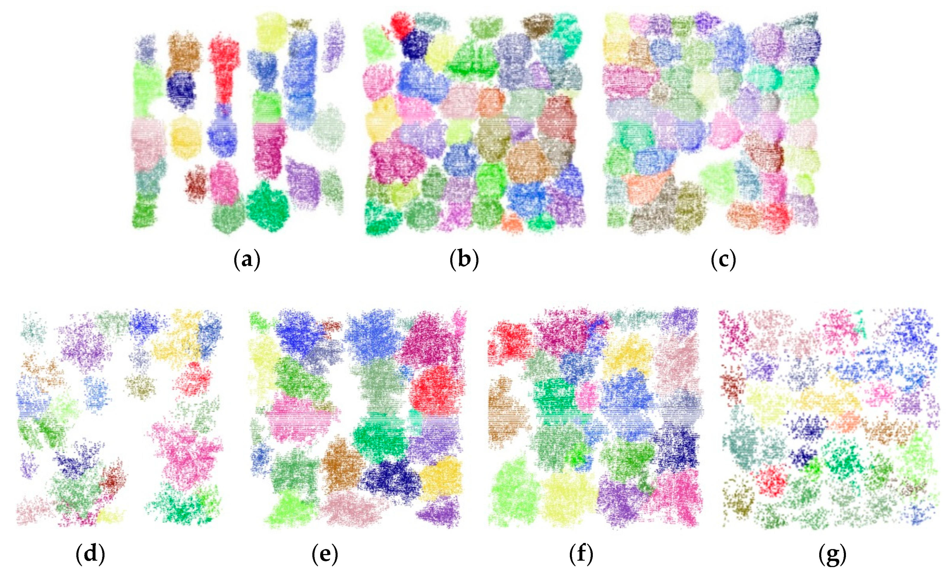
40]. Then, with the voxel-based mean shift algorithm, the non-ground UAV points were compressed and roughly segmented into a set of clusters (See
Figure 7). As shown in
Figure 7, visual inspection demonstrated that the voxel-based mean shift algorithm roughly classified the non-ground UAV voxels into well-detected and under-segmentation clusters. According to the calculated mean shift vectors that always pointed to the local density and height maxima in the non-ground UAV voxels, the clusters with distinct tree apices were classified as well detected. The well-detected clusters were then directly labeled as single trees. However, the clusters without distinct tree apex structures, labeled as under-segmentation, needed to be further processed. An under-segmentation cluster contains multiple, overlapped tree canopies or small trees. As seen in
Figure 7, the segmentation results of
Metasequoia outperformed those of
Poplar. This is because
Poplar has complex tree structures with staggered stems and irregularly-shaped canopies. On the contrary, over-segmentation phenomena existed for Poplar, as seen in
Figure 7d–g.
To further detect single trees from the under-segmentation clusters, the improved NCut segmentation method was performed. For each under-segmentation cluster, tree apices, based on the tree shape curves generated by the vertical profile information both in the x- and y-directions, were found and input to the NCut method to obtain single trees by iteratively segmenting the cluster.
Table 5 shows the single-tree segmentation results by our proposed approach. As seen in
Table 5, most single trees have been correctly segmented with an average correctness of 0.90, completeness of 0.88, and
Ef value of 0.89, respectively. For
Metasequoia (Plots 1, 2, and 3), the
Ecor values were greater than 0.96, the
Ecpt values were higher than 0.88, and the
Ef values ranged from 0.93–0.94. The quantitative results indicate that the proposed method was greatly suitable for detecting the deciduous
Metasequoia with the cone-shaped canopies, sparse branches, and leaves. For
Poplar (Plots 4, 5, 6, and 7) with the irregularly-shaped canopies and staggered-like stems, the values of
Ecor,
Ecpt, and
Ef ranged from 0.81–0.9, slightly lower than those of the
Metasequoia trees. Overall, the experiments indicate that our approach was robust to different tree species.
Moreover, according to the forest density statistics in
Table 5, we found that for
Metasequoia, slight improvements of the
Ecor values were achieved for Plots 2 and 3 with the highest forest densities of 0.060 trees/m
2 when compared to Plot 1 with a forest density of 0.032 trees/m
2. On the contrary, the
Ef values of Plots 2 and 3 were slightly lower than that of Plot 1. For
Poplar, Plots 4–6 with little differences in forest density achieved
Ef values ranging from 0.83–0.87. Compared to Plot 4 with the lowest forest density of 0.020, an improvement of the
Ecor,
Ecpt, and
Ef values of Plot 7 was achieved by 0.05, 0.02, and 0.03, respectively. This indicates that our approach was capable of processing dense forests with overlapped canopies.
4.2. Comparative Tests
A comparative test was carried out to compare our method with the marker-controlled watershed segmentation [
12]. The method was performed using LiDAR360 produced by Green Valley International (
https://www.lidar360.com/archives/5135.html), and
Figure 8 was drawn by Arcgis10.2 produced by the Environmental Systems Research Institute (ESRI).
Figure 8 and
Table 6, qualitatively and quantitatively, show the watershed segmentation results for the seven plots.
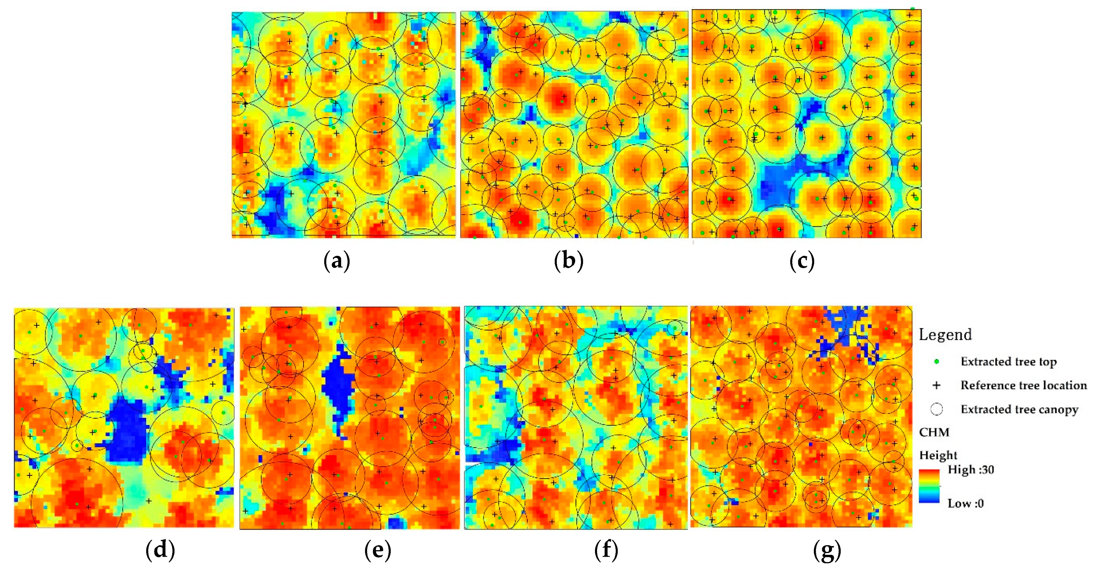
As seen in
Figure 8a–c, for the cone-shaped, orderly-arranged
Metasequoia trees, the watershed segmentation method performed very well. Accordingly, as seen in
Table 6, the values of
Ef were 0.98, 0.92, and 0.92, respectively. A few trees were over-segmented or missed. The average
Ef value of the marker-controlled watershed segmentation algorithm was slightly lower than that of our approach. This is because the watershed segmentation algorithm was sensitive to noise, which leads to staggered stems probably being misclassified into tree seed points. Moreover, the watershed segmentation algorithm detects single trees from the 2D CHM data interpolated from 3D points, which means data interpolation might decrease the accuracies of canopy segmentation and cause the unreliability of delineating crown diameters. For the
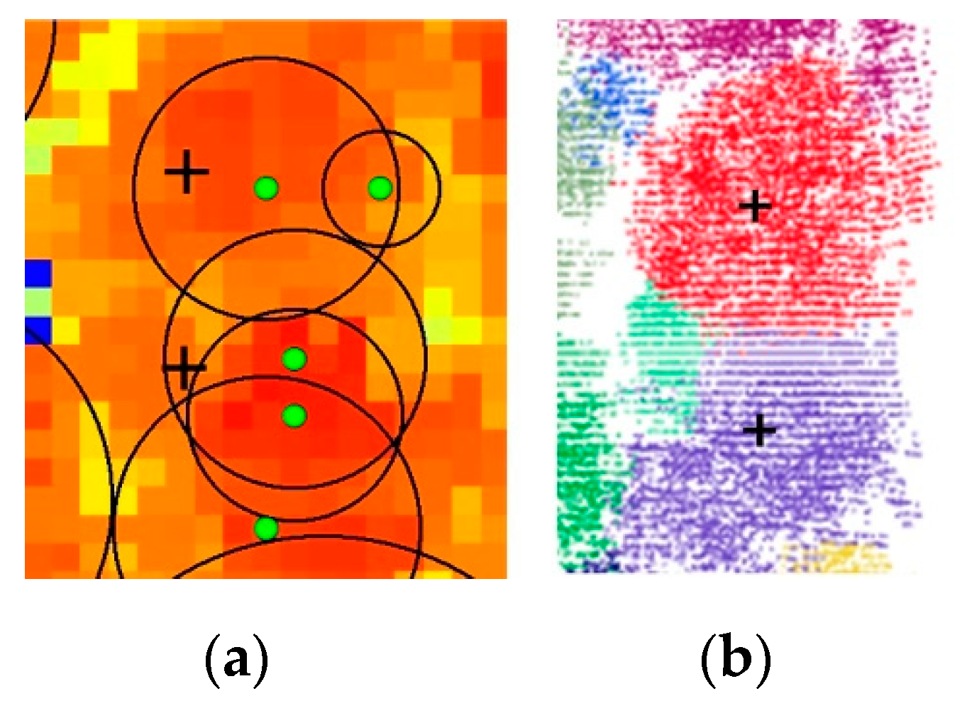
Poplar trees (Plots 4, 5, 6, and 7),
Figure 9a,b shows a close segmentation example of Plot 5 by the watershed segmentation and our proposed approach. Green dots and black circles represent tree locations and canopy radii derived from watershed segmentation, respectively, and black crosses represent reference tree locations. As seen in
Figure 9a, the single trees detected by local maxima in CHM data were over-segmented, which was mainly caused by staggered stems, and tree canopies were still overlapped with each other, indicating that the segmentation results were unsatisfactory. Quantitatively, as seen in
Table 6, the
Ecor values greatly ranged from 0.75–0.91, the
Ecpt values changed from 0.83–0.90, and the values of
Ef for the four
Poplar plots only attained 0.79, 0.80, 0.85, and 0.84, respectively. This is because the local maxima detection in 2D CHM data, which only contain height difference information, is unreliable for dealing with the trees with irregularly-shaped canopies and staggered-like branches, and thus, many
Poplar trees were over-segmented and missed.
For the Metasequoia test plots (i.e., Plots 1, 2, and 3), our proposed approach and the marker-controlled watershed segmentation method achieved similar single-tree delineation performances, both satisfactorily at delineating single trees from the cone-shaped, orderly-arranged Metasequoia forest. Moreover, for Poplar trees with irregularly-shaped canopies and staggered-like branches, the 2D CHM-based watershed segmentation method achieved unreliable results due to the loss of some tree-related information in the data interpolation. Compared to the marker-controlled watershed segmentation method, our approach was robust to forests with different tree species and forest densities by finding both local density and height maxima directly from 3D point clouds.


