Article

Modeling the Census Tract Level Housing Vacancy Rate with the Jilin1-03 Satellite and Other Geospatial Data

1
College of Resources Environment and Tourism, Capital Normal University, Beijing 100048, China
2
Beijing Advanced Innovation Center for Imaging Technology, Capital Normal University, Beijing 100048, China
3
Agricultural Information Institute, Chinese Academy of Agricultural Sciences, Beijing 100081, China
4
Department of Geography, University at Buffalo, The State University of New York, Buffalo, NY 14261, USA
*
Author to whom correspondence should be addressed.
Remote Sens. 2018, 10(12), 1920; https://doi.org/10.3390/rs10121920
Submission received: 16 October 2018 / Revised: 20 November 2018 / Accepted: 23 November 2018 / Published: 30 November 2018
(This article belongs to the Special Issue Remote Sensing of Night Lights – Beyond DMSP)

Abstract

:
The vacant house is an essential phenomenon of urban decay and population loss. Exploration of the correlations between housing vacancy and some socio-environmental factors is conducive to understanding the mechanism of urban shrinking and revitalization. In recent years, rapidly developing night-time remote sensing, which has the ability to detect artificial lights, has been widely applied in applications associated with human activities. Current night-time remote sensing studies on housing vacancy rates are limited by the coarse spatial resolution of data. The launch of the Jilin1-03 satellite, which carried a high spatial resolution (HSR) night-time imaging camera, provides a new supportive data source. In this paper, we examined this new high spatial resolution night-time light dataset in housing vacancy rate estimation. Specifically, a stepwise multivariable linear regression model was engaged to estimate the housing vacancy rate at a very fine scale, the census tract level. Three types of variables derived from geospatial data and night-time image represent the physical environment, landuse (LU) structure, and human activities, respectively. The linear regression models were constructed and analyzed. The analysis results show that (1) the HVRs estimating model using the Jilin1-03 satellite and other ancillary geospatial data fits well with the Census statistical data (adjusted R2 = 0.656, predicted R2 = 0.603, RMSE = 0.046) and thus is a valid estimation model; (2) the Jilin1-03 satellite night-time data contributed a 28% (from 0.510 to 0.656) fitting accuracy increase and a 68% (from 0.359 to 0.603) predicting accuracy increase in the estimate model of the housing vacancy rate. Reflecting socio-economic conditions, the luminous intensity of commercial areas derived from the Jilin1-03 satellite is the most influential variable to housing vacancy. Land use structure indirectly and partially demonstrated that the social environment factors in the community have strong correlations with residential vacancy. Moreover, the physical environment factor, which depicts vegetation conditions in the residential areas, is also a significant indicator of housing vacancy. In conclusion, the emergence of HSR night light data opens a new door to future microscopic scale study within cities.

1. Introduction

The phenomenon of urban shrinkage in the Great Lakes watershed region from the 1970s to 2000s in the U.S. was associated with depopulation deindustrialization [1,2,3,4]. The traditional industrial cities in this region suffered a rapid decline in industry and population, leaving behind thousands of abandoned residential houses [5,6,7,8]. As estimated by the American Community Survey (ACS), 16,842,710 vacant properties existed in the United States in 2016 [9]. In this study, we only focus on the vacant residential buildings, also called vacant houses. The causes of vacant houses are complicated and contain factors from policy, economy, and society [8]. As a typical central city in the US, Buffalo lost more than 70% of manufacturing jobs and more than 50% of the population since industry declined around the mid-1970s. As a result [10], such a large amount of abandonment properties brought serious social security and economic problems [9]. These vacant houses act as a neighborhood safety threat by creating conditions for crime. High vacancy rates reduce a city’s tax base and result in dysfunctional economy and housing markets [11,12]. Thus, vacant houses served as a symbol of city shrinkage and an indicator of community security and mental health. Relevant studies are beneficial to understanding socio-economic impact drivers and managing community revitalization.
Vacant houses are an expression of landuse (LU) change in the urban shrinkage. In previous studies, land cover (LC) and LU change are widely used to monitor the human-induced changes in the environment [13,14,15,16,17,18], especially urbanization, as the increasing impervious surface and decreasing agriculture and natural vegetated lands [19,20,21]. However, the LC change from vegetated lands to urban infrastructures in the urban expansion period is much easier to be detected from remote sensing than the minor LU change in the urban shrinking period, such as housing vacancy. Physical change in LC is reflectance-sensitive, while the LU change, such as vacancy status, makes little difference in remote sensing images. Different from developing countries, the immigration in suburbanization in developed countries is from urban to suburban instead of from rural areas, although they have similar suburban expansion phenomena. Thus, studying the inner-city areas, the origin of immigration is very essential to understanding the urban shrinking phenomenon, although detecting this minor LU change, housing vacancy, is challenging in remote sensing. In this case, we are focusing on the housing vacancy occurring at the origin of immigration in the United States, instead of LULC change in developing countries.
Putting a high priority on the vacant houses, the Census Bureau of United States started sampling field surveys to collect demographic characteristics with the housing vacancy rate (HVR), and this has occurred every 10 years since 1956. The statistical data, HVR, were annually estimated and updated based on the master address file (MAF) and the sampling field survey [22]. Although they are based on a costly door-to-door field survey, census data are still the primary data source for a variety of demographic research. However, beyond the Census statistical data, a series of studies tried to derive HVR from other data sources. Based on the relationship between vacant housing and the housing market, Lu et al. [23] calculated the commercial housing vacancy rate in Wuhan, China, using a mathematical method based on the housing price data. Rosen et al. [24] developed a cross-section model to explain natural vacancy rates, which are generated from a price-adjust model using rental price variables in 17 cities in the U.S. Using geographic information analysis, researchers simulated the housing occupancy status by integrating surrounding environmental factors. Bentley et al. [25] performed spatial distribution analysis and factor analysis in housing vacancy estimation in Detroit, MI. Wang et al. [26] measured the relationship between vacancy rate and central business district (CBD), then used a logit regression model to predict the vacancy rate, and reached the maximum value of R2, 81.5%. Huuhka et al. [9] used both geographical and statistical methods, which showed that several characteristics help in our understanding of vacancy. Silverman et al. [8] estimated the vacancy and abandonment in Buffalo, NY, using a linear regression model with various socioeconomic characteristics, and reached a maximum R2 56.8%. Although many studies have been done on HVR estimation, data in these mathematical simulation methods are from out-of-date statistical sources. Thus, they cannot meet the demand of real-time monitoring for changing cities.
As the only data source that is objective, real-time, low-cost, and easily connective with spatial data, remote sensing provides a new view from the sky and a series of real time observation datasets [27]. Emmanuel et al. [28] and Ryznar et al. [29] found that the mean value of the normalized difference vegetation index (NDVI) of residential areas was significantly correlated with HVR. Deng et al. [30] explained and modeled residential vacancy by incorporating high spatial resolution (HSR) multispectral aerial photographs and geospatial landuse datasets. The accuracy at census block and parcel level is 47.4% and 80.44%, respectively. Notably, with the development of new sensors, which are able to detect anthropogenic luminosity at night, the capability of remote sensing on human activities and associated applications has been greatly extended. Since the vacancy status of houses is caused by a lack of human activities, the night-time light (NTL) data have been used as a proxy to derive the vacancy rates. Yao et al. [31] assessed the housing vacancy in urban areas in China using nocturnal light data from the Defense Meteorological Satellite Program’s Operational Linescan System (DMSP-OLS) in 2011, and Chen et al. [32] used the same dataset to calculate HVR in 15 metropolitan areas in the U.S. with an R2 of 0.734 in 2015. However, due to the coarse spatial resolution of these datasets, existing studies have only been carried out on the national or metropolitan scale, not finer scales.
Most night-time remote sensing data in previous studies are from DMSP/OLS, and the Suomi National Polar-Orbiting Partnership’s Visible Infrared Imaging Radiometer Suite (S-NPP/VIIRS). The OLS sensor generates the low-light imaging data with a 2.7 km ground resolution. The ground instantaneous field of view at nadir is approximately 5 km and has two broad spectral bands: visible–near infrared (VNIR) and thermal infrared (TIR). With detecting clouds as the original destination, the spatial and spectral resolution of OLS-derived night-time images could not meet the requirement of diverse applications. As another valuable data source, S-NPP/VIIRS is a relatively new space-borne detector that was launched in 2012. The VIIRS images have about a 750 m ground sample distance, a 45–88-fold finer spatial resolution than DMSP, and a 14 bit radiation resolution, compared to a 6 bit digitization in DMSP [33]. Having a goal similar to DMSP/OLS, VIIRS was designed to detect moonlit clouds [34]. The byproducts of these sensors are the nocturnal images in cloud-free days. The low-light sources at night are lamps from streets, block buildings, auto headlights, public service areas, and industrial areas. These nocturnal images have been widely used for various purposes, such as socio-economic condition evaluation [35,36,37,38,39,40], GDP estimation [41,42,43,44,45], energy use and electricity consumption estimation [46,47,48,49,50], urbanization mapping [51,52,53], dynamic monitoring [54,55,56], impervious surface measurement [57,58,59], density simulation and population estimation [60,61,62,63,64,65], biogeochemical cycles and CO2 emissions simulation [66,67,68], ecological environmental impact assessment [69,70], light pollution estimation [71,72], fishery lighting detection [73,74,75,76], and fire and flammable areas mapping [77,78]. It should be noted that Ge et al. recently estimated the ghost city rate at the national scale using NPP/VIIRS [79].
Previous studies on HVR estimation using NTL remote sensing are all at very coarse scales, such as the national or metropolitan scale. However, practically, from the city manager’s perspective, studies at finer scales, such as dynamics monitoring at the urban micro level and estimating socio-economic differences within the city, are more important in urban planning to understand the mechanism of urban environment change and to make detailed city management decisions. As known, NTL can reflect urban social-economy from an objective way. Thus, finer resolution NTL sensors become pressing requirements in urban remote sensing studies. The Jilin1-03 commercial satellite, which was launched by China Changguang Satellite Technology Co., Ltd. in 2017, carried HSR night-time imaging camera and provided a new supportive data source. Equipped with sensors running at 535 km of the sun-synchronous orbit, the Jilin1-03 satellite has the capacity of video imaging, push-broom imaging, and night-time imaging. Its revisit cycle is 4.5 days when under 30 degrees sideways running. The night time imaging mode of the Jilin1-03 produces images with 12,000 × 5000 pixels, a 0.92 m spatial resolution, and three visible bands: blue, green, and red. The sub-meter level spatial resolution of this satellite imagery provides an epoch-making opportunity to research at sub-city scales. Comparison of basic information of DMSP/OLS, NPP/VIIRS, and the Jilin1-03 NTL imageries see Table 1.
With Jilin1-03 satellite night-time imagery, studies on the housing vacancy status have a chance to be performed at a finer scale. However, as a cutting-edge image data source, no HVR studies using Jilin1-03 NTL images have been explored before. The feasibility of exploring urban social-economic environment using HSR NTL images is unknown. Corresponding to these research questions, the objectives in this study, the first of its kind, is to (1) assess the feasibility of HVR estimation at the census tract level using Jilin1-03 satellite images and other ancillary geospatial data and to (2) evaluate the improvement in HVR estimation from adding fine spatial resolution (0.92 m) night-time images.

2. Study Area and Data
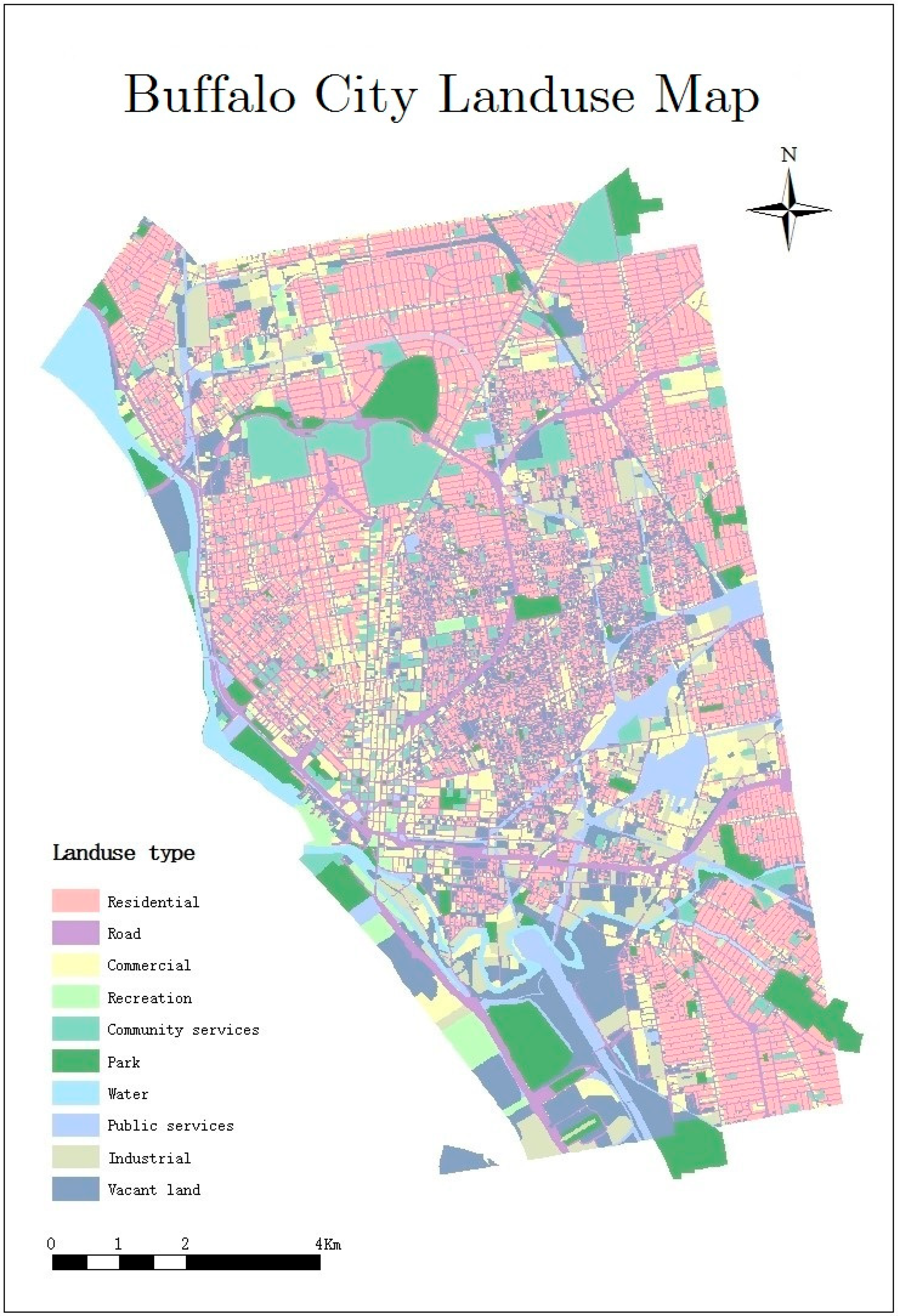
2.1. Study Area

Our study area is the City of Buffalo, a representative shrinking city located on the shores of Lake Erie in Western New York State, US. Buffalo began its decline more than a half-century ago. Based on the U.S. Census data from 1950 to 2010, the population in the city of Buffalo shrank from 580,132 to 261,310. A population loss of 318,822 amounted to about 55% of the population in 1950. Population loss and housing unaffordability forced thousands of instances of housing abandonment and housing vacancy. The city of Buffalo ranked at the third highest percentage of vacant housing in the nation, following Detroit and New Orleans. The percentage of vacant housing units reached a peak as 22.8% in 2006, when the vacant houses number was 32,637 units [80]. After that, the HVR in Buffalo decreased slightly due to the implement of revitalization policy [10]. In 2016, Buffalo ranked sixth, with an HVR of 15% [80]. This study covers 105.2 km2 of land area, including the total 77 census tracts in the city of Buffalo in 2016 [8] (Figure 1).

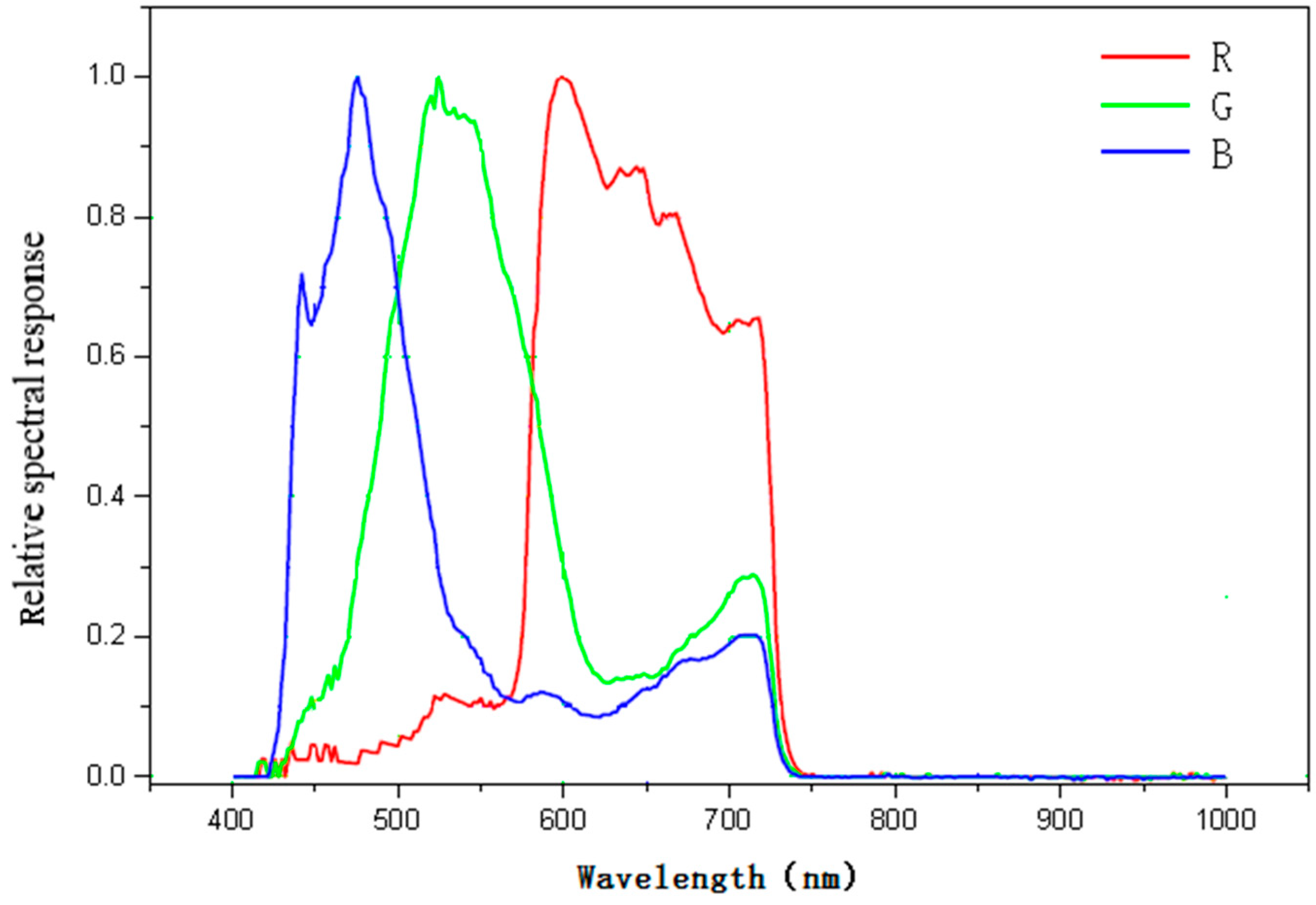
2.2. The Jilin1-03 Satellite Night-Time Image

In this study, we used a Jilin1-03 satellite night-time image with a 0.92 m spatial resolution and an 8-bit quantitative level. This image was obtained at a local time of 23:06:45 on 25 September 2017. The size of the field is 11 × 4.6 km, and our whole study area can be covered through this one shooting. The image product has been orthorectified, geometrically corrected, and mosaicked. The image was projected into the North American Datum of the 1983 Contiguous U.S.A. Albers coordinates system, which has less distortion in this area.

2.3. Other Geospatial Data

The geospatial data used include the daytime aerial digital orthoimages, parcel data, and statistical housing vacancy data from the U.S. Census Bureau five-year estimates.
The digital orthoimage product released by New York State High Resolution Statewide Digital Orthoimagery Program, New York State GIS Clearinghouse. The products for a certain county are updated once every three years. For example, for Erie County, the product was updated in 2002, 2005, 2008, 2011, 2014, and 2017. Orthoimages with a 1 ft. (30.48 cm) spatial resolution and 4 bands (natural color and near infrared) in 2017 were employed in this study. We projected orthoimages to the same coordinate system as that of Jilin1-03 satellite night-time imagery.
The parcel data are used to make landuse maps. The Buffalo parcel data contain detailed landuse information and geometric parcel boundaries in a vector format that are compiled and provided by the Office of Geographic Information Services. The newest version of parcel data is from 2016 and includes 10 landuse types in the Buffalo city: commercial, recreation, community services, residential, road, industrial, public services, vacant land, park, and water. A landuse map was derived (shown in Figure 2). Some parcels that has missing landuse data were labeled artificially by referencing Google Maps’ Street View.
The U.S. Census Bureau estimates the rental and homeowner vacancy annually, as well as the characteristics of units available for occupancy. The statistical HVR data in 2016 for census tract areas in Buffalo, Erie County, were downloaded from the U.S. Census Bureau website [80].

3. Methodology

For the purpose of HVR estimating at the census tract level, we adopted a stepwise multivariate linear regression model. Information extracted from the Jilin1-03 satellite night-time imagery, digital orthoimages, and landuse datasets is used in the modeling as explanatory variables, including three types of driving factors: the physical environment, landuse structure, and human activity. The true value of the predictive variable is the statistical housing vacancy data from the U.S. Census Bureau, which is used to construct the model.
The detailed method is in the following steps. First, the Jilin1-03 satellite night-time imagery is pre-processed. Then, explanatory variables from the Jilin1-03 satellite night-time image and other auxiliary geospatial data are extracted. Finally, the multivariate linear regression model with the above variables is used, and the accuracy is assessed. A workflow chart is shown below. (Figure 3)

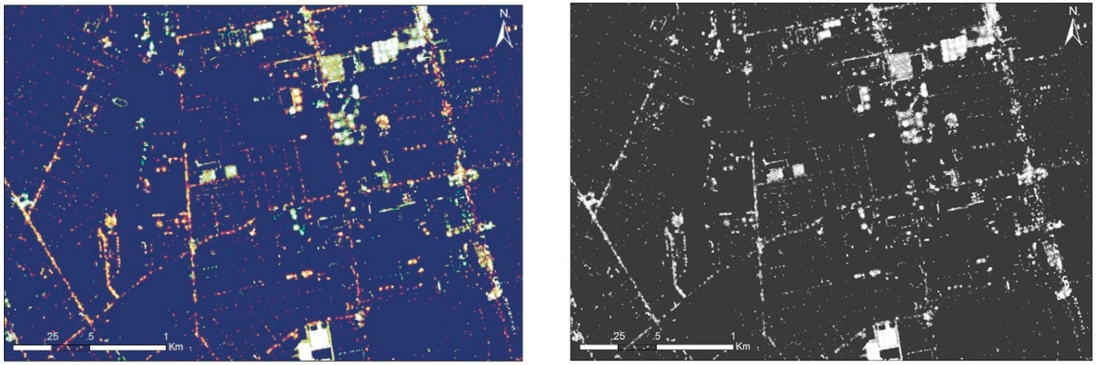
3.1. Pre-Processing of the Jilin1-03 Satellite Night-Time Image

The pre-processing of the image includes three steps: the removal of background noises, the reversion from DN value to radiance, and the conversion from RGB images to the grayscale layer. Pixels with all DN values not greater than 1 were regarded as background pixels and were set to 0, while the others were lit areas. According to the document provided by Changguang Satellite Technology Co., Ltd, which includes the spectral respond curve (Figure 4) and the conversion parameters (Table 2) from the DN value to the radiance. The conversion equation between the DN value to the radiance of three bands under the condition of a 5.6× gain and a 100 ms exposure time is
D N = a L + b
where L is the radiance in Watts m−2 sr−1 as the unit, and a and b are corresponding parameters. RGB images (Figure 5a) were converted into the radiance value of three bands. Then, we derived a single grayscale layer (Figure 4b) representing the brightness, which can reflect the emergence of human activity.

3.2. Extracting Variables from the Multi-Source Data

Three types of factors—physical environmental factors, landuse structure factors, and human activity factors—were extracted from daytime remote sensing data, geospatial landuse data, and night-time remote sending data, separately.
Physical environmental factors represent the residential physical environmental qualities during the daytime. According to Deng et al. [30], the mean lot NDVI is a consistently effective measurement both at the block group and parcel level that has a significant positive relation to the residential vacancy. Similar findings were reported at the census tract level in formal studies carried out in Detroit, MI [28,29]. To attempt to expend the usage of daytime remote sensing data in this case, we calculated the mean value and the standard deviation of NDVI, as well as the reflectance of red and near infrared bands for all residential areas in each census tract. The NDVI can be expressed as follows:
N D V I = N I R R N I R + R
where R and NIR are the reflectance of red and near infrared band.
Landuse structure factors were derived from the landuse map by calculating the following variables in each census tract: (1) the area of each landuse class, (2) the total area of each census tract, and (3) the percentage area of residential and the number of residential housing units of each census tract. Variables are involved because we consider the potential impact from the surrounding landuse types on the occupancy status of residential areas.
As urban nocturnal landscape reflects human settlements and activities, the human activity factors were proposed. For each census tract, we calculated the sum of the brightness and lit areas for each landuse type directly from the night-time image. We then obtained the average brightness and the average luminous intensity for each landuse type in a census tract, using the sum of brightness divided by the total area, and the sum of brightness divided by the lit areas, respectively.

3.3. Establishing an HVR Regression Model with Multivariate Explanatory Variables

In order to evaluate the performance of the Jilin1-03 satellite night-time data in the HVR model, we first established Model 1 without explanatory variables from the night-time imagery. Physical environmental factors and landuse structure factors were used to construct Multivariate Linear Ordinary Least Square (OLS) Regression Model 1. The processing is at the census tract level. A stepwise regression method was used. The model formula is as follows:
H V R = β j E j + γ k S k + b
where H V R is the housing vacancy rate at the census tract level, the dependent variable of the regression model; E j and S k are the physical environment and the landuse structure variables, respectively; β j and γ k are model coefficients of the physical environment and landuse structure variables, respectively; b is the constant.
For Model 2, human activity factors extracted from the Jilin1-03 satellite night-time imagery were added to Model 1. Therefore, the Model 2 formula with HSR NTL remote sensing data is
H V R = α i H i + b
where H V R is the housing vacancy rate at the census tract level, the dependent variable of the regression model; H i is the newly added human activity variable; α i is the model coefficient of the human activity variable, respectively; b is the constant. Details of all explanatory variables and their data sources are described in Table 3.

4. Results

4.1. Results of the HVR Estimation Regression Model

In this paper, combining the Jilin1-03 satellite and other geospatial data, two multivariate linear regression models at the census tract level are expressed. Model 1 has an adjusted R2 of 0.51 and an RMSE of 0.055, and Model 2, which has the factors extracted from the Jilin1-03 satellite night-time data, achieves an adjusted R2 of 0.656 and an RMSE of 0.046. Specially, the predicted R2 of Model 1 is 0.359, whereas Model 2 is 0.603. Predicted R2 is calculated by systematically removing each observation from the data set, estimating the regression equation and determining how well the model predicts the removed observation. Larger values of predicted R2 indicate models of greater predictive ability for new observations [81].
Table 4 shows the analysis result of Model 1, in which seven significant explanatory variables were selected. Three selected physical environmental variables in Model 1 were the mean value, the standard deviation of the NIR band, and the standard deviation of NDVI. Six selected landuse structure variables were the percentage area of residential in a census tract and the sum of parkland area, vacant land area, and industry area. The normalized coefficients suggest that the sum of vacant land area in a census tract has the most significant influence on residential vacancy, followed by the sum of parkland area and the mean value of the NIR band in the residential area. The p-value indicates that the mean value of NIR band, the standard deviation of NDVI, the percentage area of residential in a census tract, and the sum of parkland area and vacant land area have a significant correlation with HVR at a confidence level of 99.9%. The collinearity statistics result shows that there is no significant multicollinearity among all variables in this regression model (i.e., all with a tolerance >0.1 and a VIF < 10). Moreover, a sensitivity analysis, which can evaluate the effect from different ranges of factors on model simulation results was also carried out (see Figure 6). The sum of vacant land area and the sum of parkland area ranked as the top two. Their total ordered sensitivity index values are 0.328 and 0.282, WHICH indicated their greatest impact on the model simulation results.
The results of Model 2, which involved the Jilin1-03 satellite night-time data, are shown in Table 5. Ten significant explanatory variables selected in this model include two physical environmental variables (the mean value of NIR band and the standard deviation of NDVI), four landuse structure factors (the percentage area of residential in a census tract and the sum of parkland area, vacant land, and industry area), and four human activity variables (the average brightness of residential area, the sum brightness of residential area and vacant land, and the luminous intensity of commercial area). The normalized coefficients suggest that the luminous intensity of commercial area derived from night-time imagery ranked as the most influential variable, followed by the sum of vacant land area and parkland area derived from the landuse map. The p-value indicates that all variables are significant, above a 99% confidence level. Additionally, the collinearity statistics result shows that there is no significant multicollinearity among all variables in this regression model (i.e., all with a tolerance >0.1 and a VIF <10). Sensitivity analysis for this model (see Figure 7) shows that the luminous intensity of commercial area has the highest total ordered sensitivity index value of 0.465, the second is the sum of vacant land area (0.171), which means that the variation of these two variables has significant impacts on HVR.

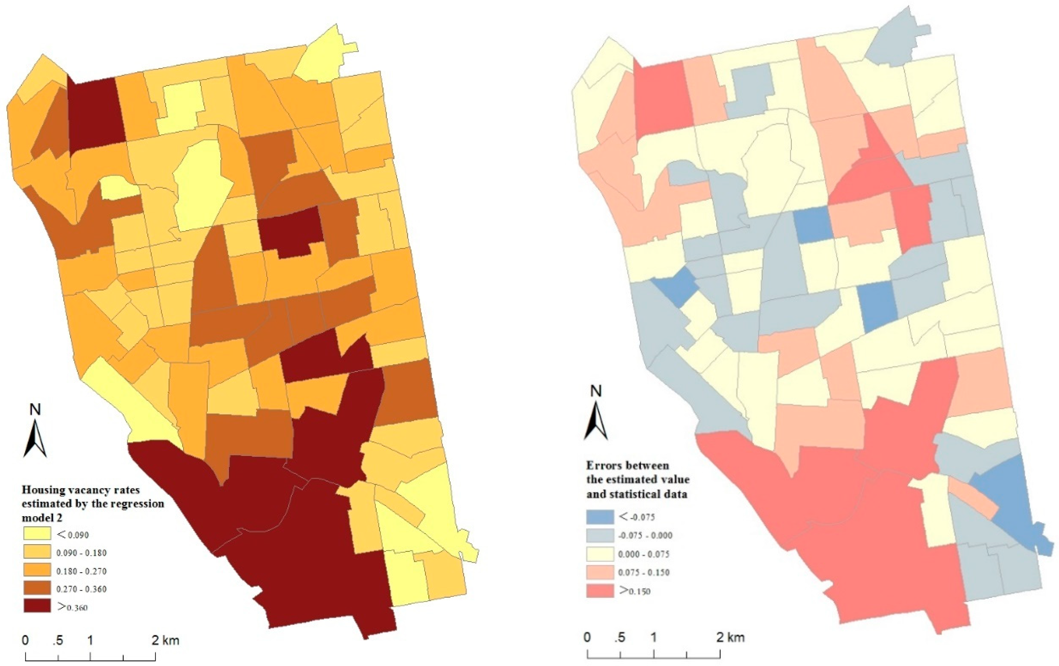
4.2. Distribution of Estimated HVR

The HVR for each census tract was estimated using Stepwise Regression Model 2 with the Jilin1-03 satellite night-time data (Equation (4)). We mapped the spatial pattern of the HVR of Buffalo (see Figure 8a). Figure 6 illustrates that the majority of the vacant houses are concentrated on the east side and in the southwest area of the city.
The spatial pattern of error was also mapped to visually examine the distribution of the error between the estimated value and the statistical data from U.S. Census Bureau (see Figure 8b). Most overestimations locate at the due east, northwest, and southwest of the city, whereas underestimations take place in the middle and southeast part. Comparing the distribution of estimated HVR, we find that overestimations mainly occur in areas with higher estimates, while underestimations are associated with lower estimates. This underfitting is probably caused by the impact from factors that are not taken into account in our model. Only linear relationships are presented in our models.

5. Discussion

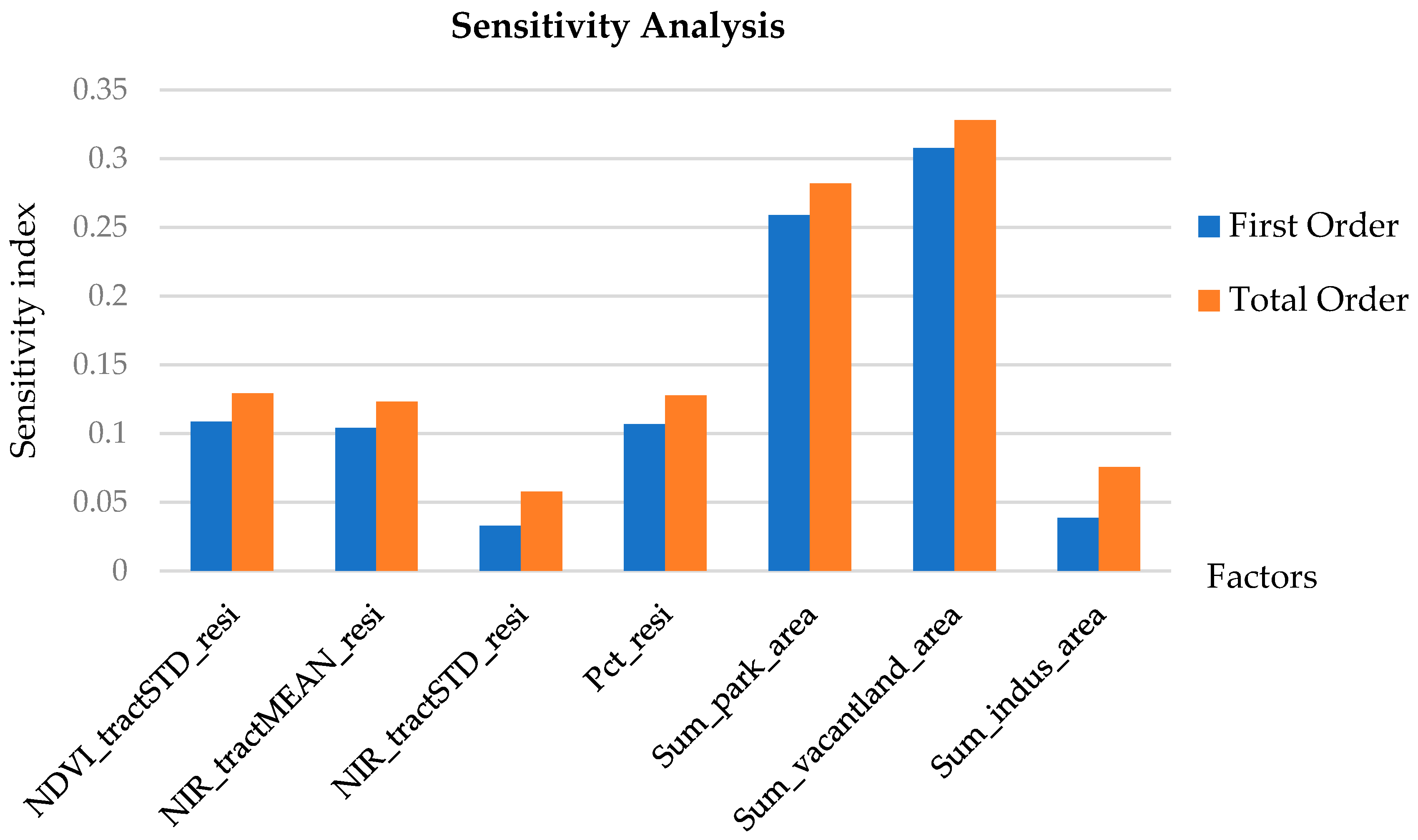
5.1. Significant Variable Analysis of the Regression Models

Among physical environmental factors derived from orthoimages, two variables were significant in both Model 1 and Model 2. The mean value of the NIR band and the standard deviation of the NDVI are negatively related to residential vacancy. Both of these represent vegetation conditions. The lawns of residential areas in the high-vacancy-rate census tracts are out of maintenance, and thus withered, and spread to impervious surfaces such as sidewalks (Figure 9b). As we know, the spectral reflectance of green plants in the near-infrared band is dramatically high. The negative relationship between the mean value of the NIR band and the housing vacancy as is expected. Similarly, vegetation withering leads to the reduction of high NDVI values, and covered impervious surfaces can cause a rise in low NDVI values. Thus, the standard deviation of the NDVI shows a negative correlation with HSR. These results prove that the physical environmental factor at the census-tract scale can express the difference in HVR. Moreover, the mean value of NIR bands and the standard deviation of NDVI can be significant indicators of housing vacancy.
Among landuse structure factors from the landuse map, which can express the social environmental characteristics of residential areas, such as infrastructure construction and the life quality of local residents, three were selected in our model. Deng et al. [30] utilized the distance from residential parcels to facilities such as nearby commercial services to study how the geospatial distribution of different landuse types affects the occupancy status of houses. In this paper, we use only the landuse type distribution within a census tract and the residential parcels characteristics (the parcel areas and housing units), to explore the relationship between landuse structures and housing vacancy. From Table 4 and Table 5, the percentage area of residential in a census tract and the sum of parkland area and industry area were negatively correlated with the residential vacancy, whereas the sum of vacant land area shows a positive correlation. These observations can partly be explained by the community attraction. A larger area of parkland and a higher percentage area of residential mean more infrastructures and better living environments. Thus, these communities are more attractive to residents. Fewer houses in this community are likely to be abandoned and left vacant. From another perspective, deindustrialization and industrial and residential suburbanization made industrial and commercial areas decline in downtown Buffalo [9]. Thousands of manufacturing jobs were lost, and thousands of people left, as industry moved out. A large amount of properties were then abandoned and became vacant. The same findings were reported by Silverman et al. [8] and Troy et al. [82].
Among the human activity factors extracted from the Jilin1-03 satellite night-time imagery, the average brightness of residential areas, the sum brightness of residential areas and vacant land, and the luminous intensity of commercial areas have significant correlations with HVR. The luminous intensity of commercial areas is the most influential variable based on the normalized coefficients in Table 5, which implies that HVRs are low in developed regions. Generally, large commercial areas are associated with economic development and higher incomes in a region [11]. Better housing affordability leads to higher housing prices and fewer vacant houses. The second significant variable is average brightness in residential areas. The higher average brightness in residential areas implies a lower HVR in the census tract. This is in line with our general knowledge that houses where no one lives are dark. The smaller sum of brightness of vacant land can be with an unsafe public security condition, hence the higher HVR in this region.

5.2. Improvements, Limitations, and Further Implications

Comparing Model 2 to Model 1, the adjusted R2 increases from 0.510 to 0.656, and the predicted R2 from 0.359 to 0.603. RMSE decreases from 0.055 to 0.046 due to the participation of the Jilin1-03 satellite night-time data. Although Model 1 has a good fitting result, an adjusted R2 of 0.510, and its predicted R2 is 0.359. This indicates a possible over-fitting problem, and the model will not predict new observations as accurately as existing data. Considering both the adjusted R2 and predicted R2, Model 2 is much better than Model 1 in fitting and predicting accuracy. Using the same training data and model complexity, explanatory variables in Model 2 have more significant and reasonable correlations with HVR. Thus, a reduced prediction bias results from adding the human activity factors.
Comparing with previous studies, the result of Model 2 is better than another HVR estimation model at the census tract level [8] and a model using daytime remote sensing data at the block group level [30]. As proven in many studies, NTL images can reflect the intensity of human activity at a large scale. Furthermore, night-time lighting information can also represent socio-economic development at the local scale. One significant phenomenon of human activities in Buffalo worth mentioning is population segregation. The African American population is highly clustered in the middle south, while population in the northwest and mid-south of Buffalo have a lower income [83]. As Buffalo lost over 70% manufacturing jobs in the 1980s, workers were not able to afford the loan and tax of their houses anymore. Thus, housing unaffordability became a serious social problem, especially for poor people in African American communities [84]. A large amount of residents moved out and their houses were taken back by banks [8,10]. On the other hand, no residents or housing buyers were available at that time, especially for the houses in lower-level communities associated with social security threats and undeveloped community services. Usually, low-income communities have less infrastructure and worse security conditions that make them unattractive [12]. Even though the housing prices are quite low in these communities, there are still many vacant houses that are difficult to sell due to a lack of attraction. Thus, the HVR is an expression of the social-economic development in a region [11] as well as night-time light. The distribution of vacant houses is highly related to the segregation and social injustice in Buffalo. Although there is only a weak relationship between a vacant house and the reflectance of its particular parcel on an NTL image, we can still find some clues from contextual information that can help to estimate the aggregated HVR on a local scale.
Since this is the first time HSR NTL imagery was used in HVR estimation, it is worth pointing out limitations in this study. First, the Jilin1-03 satellite night-time data contain two weaknesses. One is the limitation of light detection ability. Since the low light detection limit is set to 7E-7 Watt/cm2/Sr, weak lights are undetectable and useful information can be lost. Moreover, the Jilin1-03 satellite night-time imagery is not free and need to be ordered. Images of Buffalo are not archived, so the data need to be obtained through reprogramming and have a higher price. A scene of Buffalo costs about 20,000 renminbi, which equals to 2870 USD. Thus, purchasing a bunch of Jilin1-03 images for a large–area study or a multitemporal study is costly. In this study, we only used one scene, but housing vacancy is a long-term phenomenon. With a limited budget, this is the best data we could obtain in our study area. Additionally, the HVR in Buffalo is not changing rapidly. Most night-time lights, such as road lamps and parking lot lamps, are consistent during the night. Although a single image is used in this study, we can still extract useful information from it. Second, the framework regression model is simple, and some useful factors may not be included. As a linear model, the limitations of this method can cause a misinterpretation of the practical meaning of the selected variables. Furthermore, it is still a challenge to infer human–activity parameters through remote sensing. Although 54 influential factors were involved in our models, housing vacancy is highly uncertain as the consequence of human activity prediction. Additionally, our method was designed and tested in the urban area in developed countries. In developing countries, a lack of open detailed landuse maps and different driving mechanisms of housing vacancy imply that our method may not adapt to study areas in developing countries.
Future research should seek to (1) involve more variables when inversing HVR, (2) conduct multi-spectral information from the Jilin1-03 satellite data, (3) employ long-term series images of the Jilin1-03 satellite, (4) test more models and develop advanced methods to extract information from NTL images, and (5) expand the employment of the Jilin1-03 NTL data to other social applications.

6. Conclusions

To our knowledge, this is the first time HSR night-time remote sensing in HVR modeling at a sub-city scale has been performed. As a brand new dataset, Jilin1-03 was explored in a typical urban social application: HVR estimation. In a stepwise multivariate linear regression model, three driving factors derived from Jilin1-03 and other data were analyzed. The results of this study show two conclusions.
First, the HVR estimating model using the Jilin1-03 satellite and other ancillary geospatial data fits well with census statistical data. Data used to extract variables in this study can be easily obtained and updated on time. Independent from ground surveys and statistical data, the established model using remote sensing and geospatial landuse data provides an alternative method for analyzing or even predicting HVRs, especially for the census year that has no recent HVR data or reliable statistical data.
Second, the Jilin1-03 satellite night-time data contribute a 28% fitting accuracy increase to the estimation model and a 68% predicting accuracy increase, by involving night-time data in the model. The luminous intensity of commercial areas derived from the Jilin1-03 satellite was found to be the most influential variable for housing vacancy, through reflecting socio-economic conditions. The landuse structure indirectly and partially demonstrated that the social environment factors have strong correlations with residential vacancy. Moreover, the physical environment depicting vegetation conditions in the residential areas is also found to be a significant indicator of housing vacancy.
Our study is conducive to urban community management and revitalization policy formulation. The emergence of HSR night light data opens a new door to future studies on a microscopic scale. It is highly important to explore the potential of Jilin1-03 satellite HSR NTL remote sensing data.

Author Contributions

M.D. designed and completed the experiments and the draft. L.W. initiated the overall research question and fund for this project. S.Z. helped to complete the manuscript. C.S. provided research suggestions of this paper.

Acknowledgments

This work was supported by “Capacity Building for Sci-Tech Innovation—Fundamental Scientific Research Funds (025185305000/199; 025185305000/211)” and “National Natural Science Foundation of China (41828102, 41601363)”. We would like to thank the anonymous reviewers for helpful insights in improving this paper.

Conflicts of Interest

The authors declare no conflict of interest.

References

  1. Häußermann, H.; Siebel, W. Die Schrumpfende Stadt und die Stadtsoziologie; VS Verlag für Sozialwissenschaften: Wiesbaden, Germany, 1988; pp. 78–94. [Google Scholar]
  2. Martinez-Fernandez, C.; Audirac, I.; Fol, S.; Cunningham-Sabot, E. Shrinking Cities: Urban Challenges of Globalization. Int. J. Urban Reg. Res. 2012, 36, 213–225. [Google Scholar] [CrossRef] [PubMed]
  3. Pallagst, K.; Aber, J.; Audirac, I.; Cunningham-Sabot, E.; Fol, S.; Martinez-Fernandez, C.; Moraes, S.; Mulligan, H.; Vargas-Hernandez, J.; Wiechmann, T.; Wu, T. The Future of Shrinking Cities: Problems, Patterns and Strategies of Urban Transformation in a Global Context; Sae Technical Papers; University of California: Oakland, CA, USA, 2009. [Google Scholar]
  4. Nassauer, J.I.; Raskin, J. Urban vacancy and land use legacies: A frontier for urban ecological research, design, and planning. Landsc. Urban Plan. 2014, 125, 245–253. [Google Scholar] [CrossRef]
  5. Haase, D.; Haase, A.; Rink, D. Conceptualizing the nexus between urban shrinkage and ecosystem services. Landsc. Urban Plan. 2014, 132, 159–169. [Google Scholar] [CrossRef]
  6. Rall, E.L.; Haase, D. Creative intervention in a dynamic city: A sustainability assessment of an interim use strategy for brownfields in Leipzig, Germany. Landsc. Urban Plan. 2011, 100, 189–201. [Google Scholar] [CrossRef]
  7. Logan, J. Greening the Rust Belt: A Green Infrastructure Model for Right Sizing America’s Shrinking Cities. J. Am. Plan. Assoc. 2008, 74, 451–466. [Google Scholar]
  8. Silverman, R.M.; Yin, L.I.; Patterson, K.L. Dawn of the Dead City: An Exploratory Analysis of Vacant Addresses in Buffalo, NY 2008–2010. J. Urban Affairs 2013, 35, 131–152. [Google Scholar] [CrossRef]
  9. Huuhka, S. Vacant residential buildings as potential reserves: A geographical and statistical study. Build. Res. Inf. 2016, 44, 816–839. [Google Scholar] [CrossRef]
  10. Schilling, J. Blueprint Buffalo—Using Green Infrastructure to Reclaim America’s Shrinking Cities. In The Future of Shrinking Cities: Problems, Patterns and Strategies of Urban Transformation in a Global Context; The Shrinking Cities International Research Network: Leipzig, Germany, 2009. [Google Scholar]
  11. Huuhka, S.; Lahdensivu, J. Statistical and geographical study on demolished buildings. Build. Res. Inf. 2016, 44, 73–96. [Google Scholar] [CrossRef]
  12. Accordino, J.; Johnson, G.T. Addressing the Vacant and Abandoned Property Problem. J. Urban Affairs 2000, 22, 301–315. [Google Scholar] [CrossRef]
  13. Bauer, M.E.; Yuan, F.; Sawaya, K.E. Multi-temporal landsat image classification and change analysis of land cover in the twin cities (minnesota) metropolitan area. Remote Sens. Environ. 2005, 98, 317–328. [Google Scholar]
  14. Sleeter, B.M.; Sohl, T.L.; Loveland, T.R.; Auch, R.F.; Acevedo, W.; Drummond, M.A.; Sayler, K.L.; Stehman, S.V. Land-cover change in the conterminous United States from 1973 to 2000. Glob. Environ. Chang. 2013, 23, 733–748. [Google Scholar] [CrossRef]
  15. Wu, S.-S.; Qiu, X.; Wang, L. Using Semi-variance Image Texture Statistics to Model Population Densities. Am. Cartogr. 2006, 33, 127–140. [Google Scholar] [CrossRef]
  16. Wu, S.-S.; Qiu, X.; Wang, L. Population Estimation Methods in GIS and Remote Sensing: A Review. Map. Sci. Remote Sens. 2005, 42, 17. [Google Scholar] [CrossRef]
  17. Silván-Cárdenas Jose, L.; Wang, L.; Rogerson, P.; Wu, C.S.; Feng, T.T.; Kamphaus, B.D. Assessing fine-spatial-resolution remote sensing for small-area population estimation. Int. J. Remote Sens. 2010, 31, 5605–5634. [Google Scholar] [CrossRef]
  18. Deng, C.; Wu, C.; Wang, L. Improving the housing-unit method for small-area population estimation using remote-sensing and GIS information. Int. J. Remote Sens. 2010, 31, 5673–5688. [Google Scholar] [CrossRef]
  19. Pawe, C.K.; Saikia, A. Unplanned urban growth: Land use/land cover change in the Guwahati Metropolitan Area, India. Geografisk Tidskrift 2018, 118, 88–100. [Google Scholar] [CrossRef]
  20. Dewan, A.M.; Yamaguchi, Y. Land use and land cover change in Greater Dhaka, Bangladesh: Using remote sensing to promote sustainable urbanization. Appl. Geogr. 2009, 29, 390–401. [Google Scholar] [CrossRef]
  21. Acheampong, M.; Yu, Q.; Enomah, L.D.; Anchang, J.; Eduful, M. Land use/cover change in Ghana’s oil city: Assessing the impact of neoliberal economic policies and implications for sustainable fevelopment goal number one—A remote sensing and GIS approach. Land Use Policy 2018, 73, 373–384. [Google Scholar] [CrossRef]
  22. Weinberg, D.H. How the United States measures well-being in household surveys. J. Off. Stat. Stockholm 2006, 22, 113. [Google Scholar]
  23. Lu, H.; Lv, J. The research of Wuhan commercial housing vacancy rate. In Proceedings of the 2012 International Conference on Information Management, Innovation Management and Industrial Engineering, Sanya, China, 20–21 October 2012. [Google Scholar]
  24. Rosen, K.T.; Smith, L.B. The Price-Adjustment Process for Rental Housing and the Natural Vacancy Rate. Am. Econ. Rev. 1983, 73, 779–786. [Google Scholar]
  25. Bentley, G.C.; Mccutcheon, P.; Cromley, R.G.; Hanink, D.M. Race, class, unemployment, and housing vacancies in Detroit: An empirical analysis. Urban Geogr. 2015, 37, 1–16. [Google Scholar] [CrossRef]
  26. Wang, H.; Chang, C.J. Simulation of housing market dynamics: Amenity distribution and housing vacancy. In Proceedings of the 2013 Winter Simulations Conference (WSC), Washington, DC, USA, 8–11 December 2013; pp. 2749–2770. [Google Scholar]
  27. Wang, L.; Shi, C.; Diao, C.; Ji, W.; Yin, D. A survey of methods incorporating spatial information in image classification and spectral unmixing. Int. J. Remote Sens. 2016, 37, 3870–3910. [Google Scholar] [CrossRef] [Green Version]
  28. Emmanuel, R. Urban vegetational change as an indicator of demographic trends in cities: The case of Detroit. Environ. Plan. B 1997, 24, 415–426. [Google Scholar] [CrossRef]
  29. Ryznar, R.M.; Wagner, T.W. Using Remotely Sensed Imagery to Detect Urban Change: Viewing Detroit from Space. J. Am. Plan. Assoc. 2001, 67, 327–336. [Google Scholar] [CrossRef]
  30. Deng, C.; Ma, J. Viewing urban decay from the sky: A multi-scale analysis of residential vacancy in a shrinking U.S. city. Landsc. Urban Plan. 2015, 141, 88–99. [Google Scholar] [CrossRef]
  31. Yao, Y.; Li, Y. House vacancy at urban areas in China with nocturnal light data of DMSP-OLS. In Proceedings of the 2011 IEEE International Conference on Spatial Data Mining and Geographical Knowledge Services, Fuzhou, China, 29 June–1 July 2011. [Google Scholar]
  32. Chen, Z.; Yu, B.; Hu, Y.; Huang, C.; Shi, K.; Wu, J. Estimating House Vacancy Rate in Metropolitan Areas Using NPP-VIIRS Nighttime Light Composite Data. IEEE J. Sel. Top. Appl. Earth Obs. Remote Sens. 2017, 8, 2188–2197. [Google Scholar] [CrossRef]
  33. Kyba, C.C.M.; Garz, S.; Kuechly, H.; de Miguel, A.S.; Zamorano, J.; Fischer, J.; Hölker, F. High-Resolution Imagery of Earth at Night: New Sources, Opportunities and Challenges. Remote Sens. 2015, 7, 1–23. [Google Scholar] [CrossRef] [Green Version]
  34. Hillger, D.; Kopp, T.; Lee, T.; Lindsey, D.; Seaman, C.; Miller, S.; Solbrig, J.; Kidder, S.; Bachmeier, S.; Jasmin, T.; Rink, T. First-Light imagery from SuomiNPP VIIRS. Bull. Am. Meteorol. Soc. 2013, 94, 1019–1029. [Google Scholar] [CrossRef]
  35. Elvidge, C.D.; Sutton, P.C.; Ghosh, T.; Tuttle, B.T.; Baugh, K.E.; Bhaduri, B.L.; Bright, E.A. A global poverty map derived from satellite data. Comput. Geosci. 2009, 35, 1652–1660. [Google Scholar] [CrossRef]
  36. Ghosh, T.; Anderson, S.J.; Elvidge, C.D.; Sutton, P.C. Using Nighttime Satellite Imagery as a Proxy Measure of Human Well-Being. Sustainability 2013, 5, 4988–5019. [Google Scholar] [CrossRef] [Green Version]
  37. Ghosh, T. Estimation of Mexico’s Informal Economy and Remittances Using Nighttime Imagery. Remote Sens. 2009, 1, 418–444. [Google Scholar] [CrossRef] [Green Version]
  38. Doll, C.N.H.; Muller, J.P.; Morley, J.G. Mapping regional economic activity from night-time light satellite imagery. Ecol. Econ. 2006, 57, 75–92. [Google Scholar] [CrossRef]
  39. Zhou, Y.; Ma, T.; Zhou, C.; Xu, T. Nighttime Light Derived Assessment of Regional Inequality of Socioeconomic Development in China. Remote Sens. 2015, 7, 1242–1262. [Google Scholar] [CrossRef] [Green Version]
  40. Wu, R.; Yang, D.; Dong, J.; Yang, D.; Dong, J.; Zhang, L.; Xia, F. Regional inequality in China based on NPP-VIIRS night-time light imagery. Remote Sens. 2018, 10, 240. [Google Scholar] [CrossRef]
  41. Doll, C.N.H. CIESIN Thematic Guide to Night-Time Light Remote Sensing and Its Applications; Center for International Earth Science Information Network (CIESIN), Columbia University: Palisades, NY, USA, 2008. [Google Scholar]
  42. Yue, W.; Gao, J.; Yang, X. Estimation of Gross Domestic Product Using Multi-Sensor Remote Sensing Data: A Case Study in Zhejiang Province, East China. Remote Sens. 2014, 6, 7260–7275. [Google Scholar] [CrossRef] [Green Version]
  43. Qi, K.; Hu, Y.; Cheng, C.; Chen, B. Transferability of Economy Estimation Based on DMSP/OLS Night-Time Light. Remote Sens. 2017, 9, 786. [Google Scholar] [CrossRef]
  44. Zhu, X.; Ma, M.; Yang, H.; Bo, C. Modeling the Spatiotemporal Dynamics of Gross Domestic Product in China Using Extended Temporal Coverage Nighttime Light Data. Remote Sens. 2017, 9, 626. [Google Scholar] [CrossRef]
  45. Doll, C.N.H.; Muller, J.P.; Elvidge, C.D. Nighttime Imagery as a Tool for Global Mapping of Socioeconomic Parameters and Greenhouse Gas Emissions. Ambio 2000, 29, 157–162. [Google Scholar] [CrossRef]
  46. Elvidge, C.D.; Baugh, K.E.; Kihn, E.A.; Kroehl, H.W.; Davis, E.R.; Davis, C.W. Relation between satellite observed visible-near infrared emissions, population, economic activity and electric power consumption. Int. J. Remote Sens. 1997, 18, 1373–1379. [Google Scholar] [CrossRef]
  47. Letu, H.; Hara, M.; Yagi, H.; Naoki, K.; Tana, G.; Nishio, F.; Shuhei, O. Estimating energy consumption from night-time DMPS/OLS imagery after correcting for saturation effects. Int. J. Remote Sens. 2010, 31, 4443–4458. [Google Scholar] [CrossRef]
  48. Amaral, S.; Câmara, G.; Monteiro, A.M.V.; Quintanilha, J.A.; Elvidge, C.D. Estimating population and energy consumption in Brazilian Amazonia using DMSP night-time satellite data. Comput. Environ. Urban Syst. 2005, 29, 179–195. [Google Scholar] [CrossRef]
  49. Welch, R.; Zupko, S. Urbanized area energy utilization patterns from DMSP data. Photogramm. Eng. Remote Sens. 1980, 46, 201–207. [Google Scholar]
  50. Welch, R. Monitoring urban population and energy utilization patterns from satellite data. Remote Sens. Environ. 1980, 9, 1–9. [Google Scholar] [CrossRef]
  51. Imhoff, M.L.; Lawrence, W.T.; Stutzer, D.C.; Elvidge, C.D. A technique for using composite DMSP/OLS “City Lights” satellite data to map urban area. Remote Sens. Environ. 1997, 61, 361–370. [Google Scholar] [CrossRef]
  52. Lo, C.P. Urban Indicators of China from Radiance-Calibrated Digital DMSP-OLS Nighttime Images. Ann. Assoc. Am. Geogr. 2015, 92, 225–240. [Google Scholar] [CrossRef]
  53. Li, K.; Chen, Y. A Genetic Algorithm-Based Urban Cluster Automatic Threshold Method by Combining VIIRS DNB, NDVI, and NDBI to Monitor Urbanization. Remote Sens. 2018, 10, 277. [Google Scholar] [CrossRef]
  54. Small, C.; Pozzi, F.; Elvidge, C.D. Spatial analysis of global urban extent from DMSP-OLS night lights. Remote Sens. Environ. 2005, 96, 277–291. [Google Scholar] [CrossRef]
  55. Zhang, Q.; Seto, K.C. Mapping Urbanization Dynamics at Regional and Global Scales Using Multi-temporal DMSP/OLS Nighttime Light Data. Remote Sens. Environ. 2011, 115, 2320–2329. [Google Scholar]
  56. Xue, X.; Zheng, Q.; Wang, K. Delineating Urban Boundaries Using Landsat 8 Multispectral Data and VIIRS Nighttime Light Data. Remote Sens. 2018, 10, 799. [Google Scholar] [CrossRef]
  57. Elvidge, C.D.; Tuttle, B.T.; Sutton, P.C.; Baugh, K.E.; Howard, A.T.; Cristina, M.; Cristina, B.; Nemani, R. Global Distribution and Density of Constructed Impervious Surfaces. Sensors 2007, 7, 1962–1979. [Google Scholar] [CrossRef] [PubMed] [Green Version]
  58. Shao, Z.; Liu, C. The Integrated Use of DMSP-OLS Nighttime Light and MODIS Data for Monitoring Large-Scale Impervious Surface Dynamics: A Case Study in the Yangtze River Delta. Remote Sens. 2014, 6, 9359–9378. [Google Scholar] [CrossRef] [Green Version]
  59. Guo, W.; Lu, D.; Kuang, W. Improving Fractional Impervious Surface Mapping Performance through Combination of DMSP-OLS and MODIS NDVI Data. Remote Sens. 2017, 4, 375. [Google Scholar] [CrossRef]
  60. Doll, C.N.H. Population detection profiles of DMSP-OLS night-time imagery by regions of the world. Proc. Asia-Pac. Adv. Netw. 2010, 30, 190–206. [Google Scholar] [CrossRef]
  61. Sutton, P.C.; Elvidge, C.; Obremski, T. Building and Evaluating Models to Estimate Ambient Population Density. Photogramm. Eng. Remote Sens. 2003, 69, 545–553. [Google Scholar] [CrossRef]
  62. Amaral, S.; Monteiro, A.M.V.; Camara, G.; Quintanilha, J.A. DMSP/OLS night-time light imagery for urban population estimates in the Brazilian Amazon. Int. J. Remote Sens. 2006, 27, 855–870. [Google Scholar] [CrossRef]
  63. Sutton, P.; Roberts, D.; Elvidge, C.; Baugh, K. Census from Heaven: An estimate of the global human population using night-time satellite imagery. Int. J. Remote Sens. 2001, 22, 3061–3076. [Google Scholar] [CrossRef]
  64. Zeng, C.Q.; Zhou, Y.; Wang, S.X.; Yan, F.L.; Zhao, Q. Population Spatialization in China Based on Nighttime Imagery and Land Use Data. Int. J. Remote Sens. 2011, 32, 9599–9620. [Google Scholar] [CrossRef]
  65. Briggs, D.J.; Gulliver, J.; Fecht, D.; Vienneau, D. Dasymetric modelling of small-area population distribution using land cover and light emissions data. Remote Sens. Environ. 2007, 108, 451–466. [Google Scholar] [CrossRef]
  66. Milesi, C.; Running, S.W.; Elvidge, C.D.; Dietz, J.B.; Tuttle, B.T.; Nemani, R.R. Mapping and Modeling the Biogeochemical Cycling of Turf Grasses in the United States. Environ. Manag. 2005, 36, 426–438. [Google Scholar] [CrossRef] [PubMed]
  67. Meng, X.; Han, J.; Huang, C. An Improved Vegetation Adjusted Nighttime Light Urban Index and Its Application in Quantifying Spatiotemporal Dynamics of Carbon Emissions in China. Remote Sens. 2017, 9, 829. [Google Scholar] [CrossRef]
  68. Zhang, X.; Wu, J.; Peng, J.; Cao, Q. The Uncertainty of Nighttime Light Data in Estimating Carbon Dioxide Emissions in China: A Comparison between DMSP-OLS and NPP-VIIRS. Remote Sens. 2017, 9, 797. [Google Scholar] [CrossRef]
  69. Sutton, P.C. An Empirical Environmental Sustainability Index Derived Solely from Nighttime Satellite Imagery and Ecosystem Service Valuation. Popul. Environ. 2003, 24, 293–311. [Google Scholar] [CrossRef]
  70. He, C.Y.; Liu, Z.F.; Tian, J.; Ma, Q. Urban Expansion Dynamics and Natural Habitat Loss in China: A Multiscale Landscape Perspective. Glob. Chang. Biol. 2015, 20, 2886–2902. [Google Scholar] [CrossRef] [PubMed]
  71. Falchi, F.; Cinzano, P.; Duriscoe, D.; Kyba, C.C.M.; Elvidge, C.D.; Baugh, K.; Portnov, B.A.; Rybnikova, N.A.; Furgoni, R. The new world atlas of artificial night sky brightness. Sci. Adv. 2016, 2, e1600377. [Google Scholar] [CrossRef] [PubMed] [Green Version]
  72. Jiang, W.; He, G.; Long, T.; Wang, C.; Ni, Y.; Ma, R. Assessing Light Pollution in China Based on Nighttime Light Imagery. Remote Sens. 2017, 9, 135. [Google Scholar] [CrossRef]
  73. Rodhouse, P.G.; Elvidge, C.D.; Trathan, P.N. Remote sensing of the global light-fishing fleet: An analysis of interactions with oceanography, other fisheries and predators. Adv. Mar. Biol. 2001, 39, 261–278. [Google Scholar]
  74. Cho, K.; Ito, R.; Shimoda, H.; Sakata, T. Technical note and cover Fishing fleet lights and sea surface temperature distribution observed by DMSP/OLS sensor. Int. J. Remote Sens. 1999, 20, 3–9. [Google Scholar] [CrossRef]
  75. Waluda, C.M.; Trathan, P.N.; Elvidge, C.D.; Hobson, V.R.; Rodhouse, P.G. Throwing light on straddling stocks of Illex argentinus: Assessing fis. Can. J. Fish. Aquat. Sci. 2010, 59, 592–596. [Google Scholar] [CrossRef]
  76. Zhang, X.; Saitoh, S.I.; Hirawake, T. Predicting potential fishing zones of Japanese common squid (Todarodes pacificus) using remotely sensed images in coastal waters of south-western Hokkaido, Japan. Int. J. Remote Sens. 2016, 38, 1–18. [Google Scholar] [CrossRef]
  77. Theobald, D.M.; Cova, T.J.; Sutton, P.C. Exurban Change Detection in Fire-Prone Areas with Nighttime Satellite Imagery. Photogramm. Eng. Remote Sens. 2004, 70, 1249–1257. [Google Scholar]
  78. Elvidge, C.D.; Hobson, V.R.; Baugh, K.E.; Dietz, J.B.; Shimabukuro, Y.E.; Krug, T.; Novo, E.M.L.M.; Echavarria, F.R. DMSP-OLS estimation of tropical forest area impacted by surface fires in Roraima, Brazil: 1995 versus 1998. Int. J. Remote Sens. 2001, 22, 2661–2673. [Google Scholar] [CrossRef]
  79. Ge, W.; Yang, H.; Zhu, X.; Ma, M.; Yang, Y. Ghost City Extraction and Rate Estimation in China Based on NPP-VIIRS Night-Time Light Data. ISPRS Int. J. Geo-Inf. 2018, 7, 219. [Google Scholar] [CrossRef]
  80. Housing Vacancies and Homeownership (CPS/HVS). Available online: https://www.census.gov/housing/hvs (accessed on 28 September 2017).
  81. The Minitab 17 Support Website. Available online: http://support.minitab.com/en-us/minitab/17/topic-library/modeling-statistics/regression-and-correlation/goodness-of-fit-statistics/r-squared/#what-is-predicted-r-squared (accessed on 30 October 2018).
  82. Troy, A.R.; Grove, J.M.; O’Neildunne, J.P.; Pickett, S.T.; Cadenasso, M.L. Predicting opportunities for greening and patterns of vegetation on private urban lands. Environ. Manag. 2007, 40, 394–412. [Google Scholar] [CrossRef] [PubMed]
  83. Daniel, T. The persistence of segregation in Buffalo, New York: Comer vs. Cisneros and geographies of relocation decisions among low-income black households. Urban Geogr. 2006, 27, 20–44. [Google Scholar]
  84. Li, Y. The dynamics of residential segregation in Buffalo: An agent-based simulation. Urban Stud. 2009, 46. [Google Scholar]
Figure 1. Study area.
Remotesensing 10 01920 g001
Figure 2. Landuse map of Buffalo derived from parcel data.
Remotesensing 10 01920 g002
Figure 3. Methodology flowchart.
Remotesensing 10 01920 g003
Figure 4. The RGB relative spectral response of the camera on the Jilin1-03 satellite.
Remotesensing 10 01920 g004
Figure 5. The Jilin1-03 satellite night-time image with (a) RGB bands and the (b) grayscale layer.
Remotesensing 10 01920 g005
Figure 6. Sensitivity analysis of Stepwise Multivariate Linear Regression Model 1 (without Jilin1-03 satellite NTL data).
Remotesensing 10 01920 g006
Figure 7. Sensitivity analysis of Stepwise Multivariate Linear Regression Model 2 (with Jilin1-03 satellite NTL data).
Remotesensing 10 01920 g007
Figure 8. A distribution map of (a) the estimated HVR in Buffalo; (b) differences between the estimated value from our model and the Census Bureau statistical data.
Remotesensing 10 01920 g008
Figure 9. (a) An occupied house in Buffalo, NY. (b) A vacant house in Buffalo, NY. Photos were taken in 2016 by Shengyuan Zou.
Remotesensing 10 01920 g009
Table 1. Basic information of DMSP/OLS, NPP/VIIRS, and the Jilin1-03 NTL imageries.
ParametersDMSP/OLSNPP/VIIRSJilin1-03 Commercial Satellite
Platform operatorU.S. Air ForceNOAA/NASAChangguang Satellite Technology Co., Ltd
Data producer NOAA/NCEI (former NGDC)NOAA/NCEIChangguang Satellite Technology Co., Ltd
Launch year197620112017
Orbital height/km850827535
Spatial resolution/m10003750.94
Grey quantization level/bit8148
UnitDNWatt/m2/Sr for swath data, nano-Watt/cm2/Sr for composite dataWatt/m2/Sr
Data availabilityAnnual average NTL products can be downloaded for free. Monthly average and daily products need to be ordered.Annual and Monthly average NTL products, and some daily mosaic can be downloaded for free.Need to pay for the order.
Table 2. The Jilin1-03 satellite parametric for converting DN value to radiance (Watts m−2 sr−1).
Parametersab
R9681.000−4.730
G5455.000−3.703
B2997.000−4.471
Table 3. Explanatory variables of the multivariate linear regression models.
Factor TypeExplanatory VariablesDescription
Physical environmental factors from digital orthoimageNDVI_tractMEAN_resiMean NDVI in residential area
NDVI_tractSTD_resiStandard deviation NDVI in residential area
NIR_tractMEAN_resiMean value of NIR band in residential area
NIR_tractSTD_resiStandard deviation of NIR band in residential area
R_tractMEAN_resiMean value of R band in residential area
R_tractSTD_resiStandard deviation of R band in residential area
Landuse structure factors from parcel dataSumarea_landusetypeArea of residential/commercial/recreation/
road/community services/public services/industrial/park/vacant land
CensusTract_areaArea of the census tract
Pctarea_resiPercentage area of residential in a census tract
Countparcel_resiHousing units in residential area
Human activity factors from Jilin1-03 satellite NTL image (new added in model 2)Sum_landuse typeSum brightness of residential/commercial/recreation/
road/community services/public services/industrial/park/vacant land
Avg_landusetypeAverage brightness of residential/commercial/recreation/
road/community services/public services/industrial/park/vacant land
Litarea_landuse typeLit areas of residential/commercial/recreation/
road/community services/public services/industrial/park/vacant land
Intensity_landuse type luminous intensity of residential/commercial/recreation/
road/community services/public services/industrial/park/vacant land
Table 4. Stepwise Multivariate Linear Regression Model 1 (without Jilin1-03 satellite NTL data).
Factor TypeExplanatory VariablesCoefficientNormalized Coefficientp-ValueToleranceVIF
Physical environmental factorsConstant1.023
NDVI_tractSTD_resi−0.100−0.4523.403 × 10−5 ***0.6201.613
NIR_tractMEAN_resi−0.002−0.5442.069 × 10−6 ***0.5861.707
NIR_tractSTD_resi−0.004−0.2161.711 × 10−2 *0.8261.211
Landuse structure factorsPct_resi−0.191−0.4184.033 × 10−5 ***0.7091.411
Sum_park_area−0.000−0.7259.853 × 10−8 ***0.4342.303
Sum_vacantland_area0.0000.8606.414 × 10−6 ***0.2084.804
Sum_indus_area−0.000−0.3641.209 × 10−2 **0.3233.092
R2 = 0. 556; Adjusted R2 = 0.510; Predicted R2 = 0.359; Standard error = 0.055. * p < 0.05, ** p < 0.01, *** p < 0.001.
Table 5. Stepwise Multivariate Linear Regression Model 2 (with Jilin1-03 satellite NTL data).
Factor TypeExplanatory VariablesCoefficientNormalized Coefficientp-ValueToleranceVIF
Physical environmental factorsConstant0.896
NDVI_tractSTD_resi−1.128−0.5114.860 × 10−7 ***0.5681.762
NIR_tractMEAN_resi−0.002−0.3921.786 × 10−4 ***0.4872.055
Landuse structure factorsPct_resi−0.349−0.7471.103 × 10−9 ***0.4322.315
Sum_park_area−0.000−0.7744.496 × 10−10 ***0.4272.339
Sum_vacantland_area0.0001.0958.960 × 10−8 ***0.1446.963
Sum_indus_area−0.000−0.5892.670 × 10−5 ***0.2793.582
Human activity factorsAvg_resi−3338.169−0.5169.146 × 10−5 ***0.3093.234
Sum_resi0.0050.3488.501 × 10−3 **0.2873.348
Sum_vacantland0.000−0.3013.376 × 10−3 **0.4822.077
Intensity_commercial−16.135−2.0009.192 × 10−3 **0.8521.174
R2 = 0. 703; Adjusted R2 = 0.656; Predicted R2 = 0.603; Standard error = 0.046. * p < 0.05, ** p < 0.01, *** p < 0.001.

