Article

Inversion of Nearshore X-Band Radar Images to Sea Surface Elevation Maps

School of Mechanical Engineering, Tel Aviv University, Tel Aviv 6997801, Israel
*
Author to whom correspondence should be addressed.
Remote Sens. 2018, 10(12), 1919; https://doi.org/10.3390/rs10121919
Submission received: 28 September 2018 / Revised: 14 November 2018 / Accepted: 28 November 2018 / Published: 30 November 2018
(This article belongs to the Section Ocean Remote Sensing)

Abstract

:
A new method to invert X-band radar images for linear shoaling conditions is proposed. The commonly used approach for this type of inverse problems is the Fourier transform. Unlike in deep water conditions, in the shoaling region, waves are modulated both in terms of wavelength and amplitude. However, Fourier analysis assumes spacial and temporal periodicity, and homogeneity limiting its applicability to this region. In order to overcome these limitations, a wavelet based technique is developed. The proposed technique treats every spatial radar image within the time sequence individually, so no information on the dispersion relation is required. For validation purposes, surface elevation range-time shoaling realizations based on the mild slope equation are prepared. A radar imaging model including tilt and shadowing modulations, speckle noise, and the radar equation is applied to these realizations to provide modeled grazing incidence radar images. The inversion process starts with the application of the continuous wavelet transform independently for each spacial image. The procedure continues with employing a successive range independent modulation transfer function to the wavelet spectra in the wavenumber domain. Then, after a phase shift correction, an inverse continuous wavelet transform is applied. The procedure is finalized by a calibration of the retrieved maps. After the calibration, a thorough comparison between the original and the reconstructed surface elevations is performed. It shows high efficiency of the proposed method in treating wave number and amplitude modulated signals, as well as in addressing local phase shifts due to tilt modulation and noise contamination. The new inversion method is proven to have high accuracy in inhomogeneous conditions. It shows high potential to be implemented for individual wave reconstruction using real aperture radars.

Graphical Abstract

1. Introduction

Incoherent nautical X-band radars have been increasingly used for oceanographic measurements in the last decades. They have several advantages with respect to other measurement tools. First, their use is not limited by daylight conditions, as the use of some optical remote sensing instruments is. Second, radar measurement costs are generally lower than in-situ measurement ones. Finally, nautical radars are multipurpose tools that can be used simultaneously for navigational needs and for the determination of sea state parameters. As remote sensing tools, radar images provide significant coverage. Their ability to probe continuously in time enables the study of both the spatial and temporal evolution of the sea surface elevation with reasonably good resolution.
Historically, navigational radars were constructed to detect solid objects whilst the signals from the sea surface were just attributed to the sea clutter and hence, considered to be noise. Later, it was understood that this clutter contains useful information, and the related signals can be interpreted to retrieve sea state parameters, such as directional wave spectra [1,2], currents [3], and local bathymetry [4], as well as some meteorologic conditions, such as rain intensity [5], and sea surface winds [6].
By following a two-scale model of the radar backscatter [7,8], long energy-carrying waves become distinguishable on the radar images due to the hydrodynamical and geometrical modulations of the radar signal caused by the rough sea surface. Shadowing and tilt geometrical modulations are considered to be the main imaging mechanisms for grazing incidence [9,10]. Shadowing manifests as a partial occultation in long wave profiles. Tilt modulation arises as a result of changes in the local effective incidence angle, whilst hydrodynamic modulation is due to an uneven distribution of the resonating ripples density along the long wave profiles.
Due to the above mechanisms, a reconstruction procedure is required to obtain the original surface elevation from a radar image. Surface elevation maps are commonly inverted from radar image sequences using the technique proposed in [9]. In this paper, we refer to this work as the conventional method of radar image inversion. Their main idea was to use a dispersion relation shell filter in a 3D Fourier space and to subsequently apply an empirical modulation transfer function in order to fit the spectrum of modulations to the actual wave spectrum. In addition, imaging mechanisms shift the measured sea wave phases. For the abovementioned geometric modulations, the phase shift between the original surface elevation and its radar image is constant and equal to π / 2 [11]. In [12], the accuracy of the method for 2D radar images was analyzed and found to be approximately 15 % of the significant wave height for a wide range of wind sea states. In [13], a novel successive cancellation based method was proposed to avoid leakage in the spectral domain. It was also pointed out there that, due to the uniform sampling of the sea surface in radar images, the correspondent components in a wave number-frequency domain cannot always strictly satisfy the dispersion relation, which results in inaccurate wave retrieval.
As for the signal processing approach for non-stationary or non-homogeneous data, several methods have been developed in the past few decades, such as the windowed Fourier transform and, more recently, the wavelet transform [14]. The latter enables localization in the space or time-frequency domain through translation and dilation of the so-called mother wavelet. It is recognized as a powerful tool for non-homogeneous signal and image processing. Lately, it has been used for accurate local directional spectra estimation in the transition from deep to intermediate waters (e.g., [15,16,17,18]). However, although a number of attempts to improve the performance of the conventional method have been done (see e.g., [19]), little attention has been paid to the validation and cross-verification of the method in inhomogeneous nearshore environments.
The focus of this paper is to give an alternative to the existing inversion techniques in order to account for the inhomogeneity of the wavefield nearshore, in particular, due to wave shoaling effects and shadowing, and to validate its quality by means of stochastic simulations. Here, only linear shoaling, which results in wavelength shortening and amplitude modulation, is considered. The new technique can increase the quality of radar-derived surface elevations in comparison to in-situ point measurements, both for mean parameters and for individual waves. Among the advantages of the new method, is its ability to treat the whole image of the nearshore area as is, without the need to apply windowing or a dispersion relation shell filter. To simplify the validation and visualization purposes, only 1D spatial cases are presented. Additionally, considering that all of the inhomogeneous properties, both of wavefields and radar imaging, are much stronger in range than in azimuth, it is important to start from 1D cases and investigate them separately. It is also important to notice that the conventional method’s performance in 1D has not been attentively investigated so far. Some considerations about this topic, together with adaptation of the algorithm to 1D shoaling cases, are given in Appendix B.
The paper is organized as follows: Section 2 describes the realization of a wavy surface for linear shoaling conditions, both for monochromatic waves and for a JONSWAP (JOint North Sea WAve Project) spectra. Section 3 introduces the wavelet analysis used in the work. Section 4 briefly describes imaging mechanisms that are important for nearshore X-band radar imaging, including tilt and shadowing modulation, radar equations, and speckle noise, while, in Section 5, the application of those imaging mechanisms to simulated data is presented. The novel inversion procedure is given in Section 6. An error analysis depending on the shadowing probability and noise levels is performed in Section 7. The paper is finalized by some conclusions and future improvements of the proposed inversion technique in Section 8.

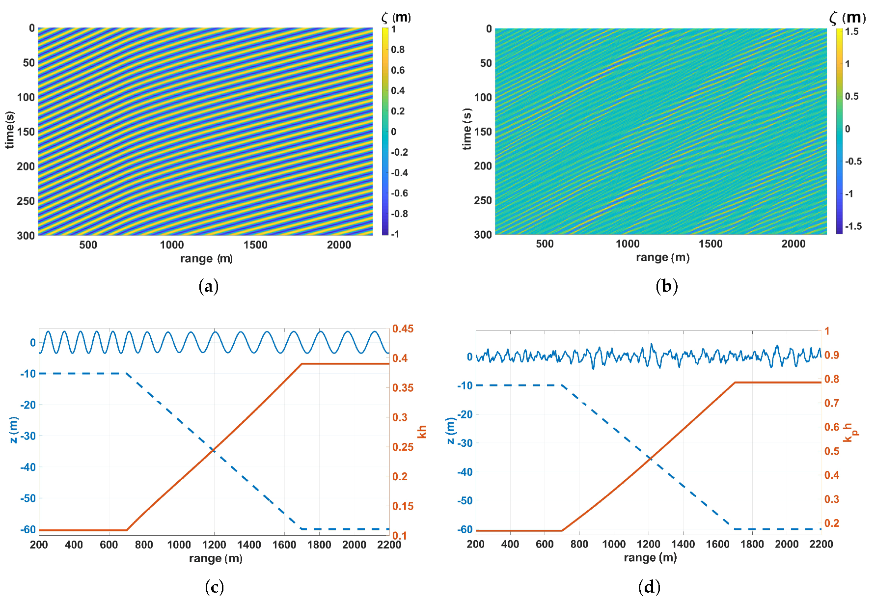
2. Inhomogeneous Sea Surface Simulation

In this section, simulations of the sea surface are described, and the information regarding bathymetry and initial conditions for every simulation is presented. First, it is necessary to discretize the wavefield into a number of bins, set the initial amplitude values, and define the bathymetry used in the simulation. It is also necessary to specify the discretization in space and time, Δ x and Δ t , to define the sea surface elevation. All of the simulation parameters are summarized in Table 1. The 1D sea surface for linear shoaling conditions can be expressed as a function of time and space in the following manner:
ζ x , t = j = 1 N a j x e i ω j t 0 x k j ξ d ξ + φ j ,
where ζ ( x , t ) is the surface elevation, a j is the amplitude of the wave component with angular frequency ω j and wave number k j that is uniformly distributed over [ 0 , 2 π ) initial random phase φ j . Throughout the paper, the units for the angular frequency and the wave number are fixed to r a d / s and r a d / m , respectively, unless otherwise stated. The angular frequency and wave number satisfy the dispersion relation
ω j 2 = g k j ( x ) tanh k j ( x ) h ( x ) ,
which is used to define the wave number k j x as a solution of Equation (2) at every point in the spatial domain. It is important to notice that, within the linear theory framework, the angular frequency of a monochromatic wave remains constant in space by virtue of the wave conservation law [20].
In order to describe linear shoaling of the wave field, the one dimensional mild slope equation [21] is used:
a j ( x ) a j ( x ) = C g , j ( x ) 2 C g , j ( x ) ,
where C g , j is the corresponding group velocity, which, in linear theory, is expressed as
C g , j ( x ) = 1 2 C j ( x ) 1 + 2 k j ( x ) h ( x ) sinh ( 2 k j ( x ) h ( x ) )
with C j ( x ) = ω j / k j ( x ) describing the phase velocity. Equation (3) can be solved for the wave amplitude
a j ( x ) = a j ( 0 ) C g , j ( 0 ) C g , j ( x ) ,
where a j ( 0 ) = 2 ω j 1 / 2 Δ ω ω j + 1 / 2 Δ ω S ( ω ) d ω 1 / 2 is the initial value of the amplitude for a JONSWAP spectrum [22] or just a fixed value of the monochromatic wave amplitude. Equation (5) is a direct consequence of the energy flux conservation.
Wolfram Mathematica software was used to simulate the sea surface as a function of space and time. Wave number values for certain depths were obtained using Equation (2). Integrals of the wave number in space 0 x k j ξ d ξ were obtained numerically. Examples of sea surface elevation realizations both for monochromatic wave and JONSWAP spectrum are shown in Figure 1.
For shoaling waves simulations, it is convenient to define the origin of the spatial coordinates in deep water at sea level. For radar image simulations, it is more common to work with the range coordinates, which correspond to the distance between the radar antenna projection to the plane z = 0 and a point of interest on the sea level. This distance is denoted as “range” in the figures below, whilst in formulas, the standard notation of x-coordinate is employed.

Linear Shoaling for Monochromatic Waves and Spectra

In the shoaling region, as a first approximation, the energy flux in the direction of the wave propagation E C g is conserved with the wave energy E a 2 . When the wave field propagates into intermediate waters, wavelengths start shortening, the group velocity changes, and therefore, the wave amplitude evolves in order to conserve the energy flux (see Figure 2). It can be seen that the monochromatic wave amplitude (Figure 2a) initially decreases as a consequence of the increase in group velocity in intermediate waters before entering shallower waters. The significant wave height depends on the wave amplitudes at all frequencies, which start shoaling in different depths; therefore, the peak wave amplitude and H s behave differently (Figure 2b).

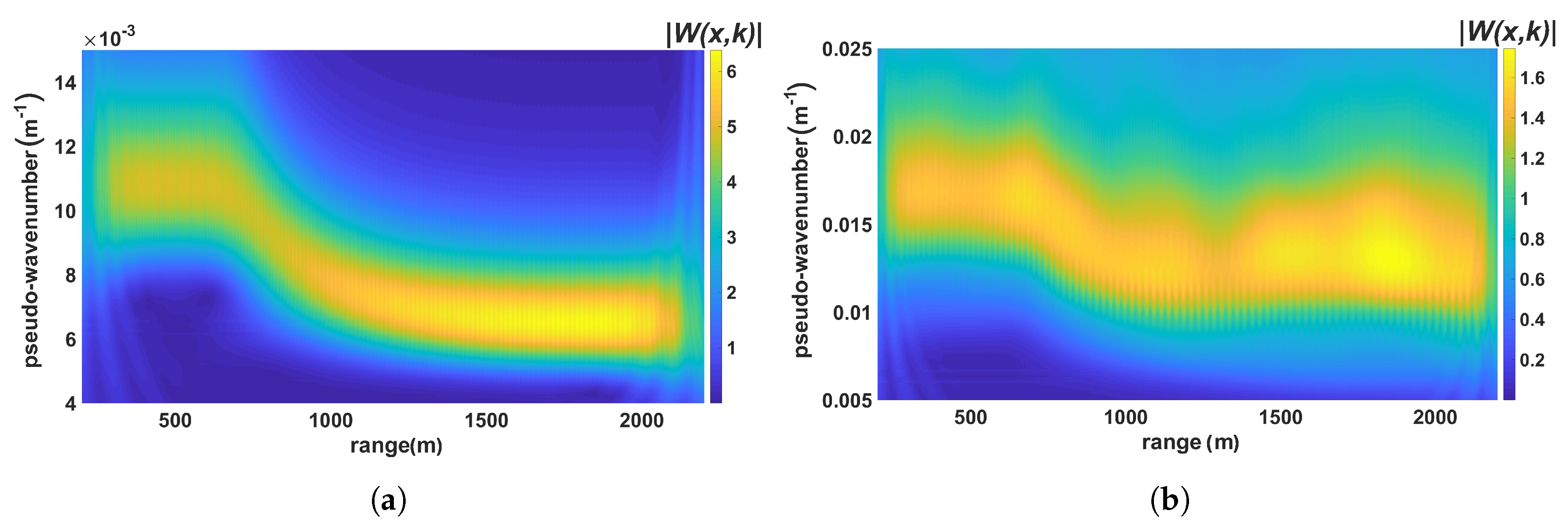
3. Wavelet Analysis of the Simulated Data

The continuous wavelet transform (CWT) can represent a signal, not only in frequency/wave number but also in the time/space domain. The CWT is defined as follows [23]:
W [ f ( x ) , ψ ( x ) ] ( a , b ) = a 1 / 2 R f ( x ) ψ * x b a d x .
Here, f ( x ) L 2 ( R ) is an initial signal, ψ is the mother wavelet, b is a coordinate shift, a is a scaling factor ( a > 0 ), and the asterisk denotes the complex conjugate. The mother wavelet is defined by assuming that ψ L 2 ( R ) and that the admissibility condition is satisfied:
2 π R | ξ | 1 | ψ ^ ( ξ ) | d ξ < ,
or, equivalently, R ψ ( ξ ) d ξ = 0 . To generate doubly indexed families of wavelets from the mother wavelet ψ , dilations and translations are added:
ψ a , b ( x ) = a 1 / 2 ψ x b a .
The normalization of the wavelet is chosen so that ψ a , b L 2 ( R ) = ψ L 2 ( R ) = 1 for all a and b.
In the water wave applications, the Morlet mother wavelet ψ ( x ) = π 1 / 4 e i ξ 0 x e ξ 0 2 / 2 e x 2 / 2 is usually used. The constant ξ 0 is chosen so that the ratio of the highest to the second highest maximum of ψ is approximately 1 / 2 , i.e., ξ 0 = π [ 2 / ln 2 ] 1 / 2 5 . 3364 ; in practice, ξ 0 = 5 is often taken. In other words, the Morlet wavelet is a complex wavelet whose real part is simply the harmonic function cos ( 5 x ) with a Gaussian envelope.
Traditionally, wavelet spectra are plotted as functions of the scaling factor a. For the following analysis, a definition of the pseudo wave number is needed. So, if K c is the central wave number of the mother wavelet, then the pseudo-wave number is defined as
K a = K c a · Δ x .
Here, K c = ξ 0 5 . To reduce the computational costs, the traditional definition of the CWT is slightly changed to rewrite Equation (6) using the identity W ( a , b ) = F 1 F { W ( a , b ) } ( F is a Fourier transform), which results in the following:
W [ f ( x ) , ψ ( x ) ] ( a , b ) = a 2 π R f ^ ( ω ) ( ψ ^ ) * ( a ω ) e i ω b d ω .
Formula (9) is widely used in different types of software and is called the Continuous Wavelet Transform with Fourier Transform (CWTFT) and is the one used in this paper. The results of the CWTFT application to the original images in Figure 1 are given in Figure 3.

4. Basic Imaging Mechanisms—A Literature Summary

As mentioned in the introduction, geometrical modulations are considered to be dominant in incoherent X-band radar imaging. For the grazing incidence, some additional imaging mechanisms start to be important. For nearshore radars, the local incident angle ψ also changes from a fairly small angle to almost π / 2 , adding significant inhomogeneity to the resulting image due to the radar equation and a range-dependent shadowing effect.
The hydrodynamic modulation is weaker than the other two [7,24]; therefore, it is not considered in this work.

4.1. The Radar Equation

The classical form of the radar equation (see, e.g., [25]) gives the received power P r as
P r = P t G t A e σ 16 π 2 R 4 ,
where P t is the transmitted power (W), G t is the antenna gain coefficient, R is the distance (m), A e is the antenna effective aperture area (m2), and σ is the target cross-section (m2).
When the same antenna is used to both transmit and receive, the transmitting gain G t and the effective receiving aperture A e are related by G t = 4 π A e / λ e m 2 , where λ e m is the length of the radar electromagnetic wave. Hence, everything on the right-hand-side of the Equation (10), except for σ and R 4 , can be included as a constant.
For our purposes, Equation (10) is represented in terms of the intensity I ( r ) I 0 / R 3 (here, I 0 is a reference intensity), since the pixel size is equal to R Δ r Δ ϕ and grows with R ( Δ r and Δ ϕ are the range and the azimuthal resolution, respectively). However, for the 1D case the range dependence on the pixel size can be disregarded.

4.2. Shadowing

Shadowing modulation is a partial occultation in long wave profiles. This is due to the fact that the tangent electromagnetic rays cannot penetrate significantly into the area of a long wave profile situated under the ray between the tangent point and next intersection points (Figure 4). Generally speaking, shadowing can not be considered a purely geometrical effect, especially for the vertical polarization of electromagnetic signals [26]. For horizontal ones, geometric shadowing is assumed to be a rather good approximation.
There are several ways to calculate the shadowing mask for a given realization of the surface elevation and probing geometry. For a discretized sea surface, an approach based on the comparison of the local incidence angles is employed. For a given realization of the surface elevation ζ ( x , t ) , the local incidence angles are defined as β ( x , t ) = arctan x H r ζ ( x , t ) , where H r is the radar installation height. Then, for a fixed time instance t , the shadowing condition depicted in Figure 4 is applied to each range point x i : β ( x k , t ) β ( x i , t ) , k : i < k N x . If, for any point x k , the condition is satisfied, the corresponding surface point ζ ( x k , t ) is marked as shadowed using an indicator (shadowing mask):
χ ( x , t ) = 1 , if ζ ( x , t ) is shadowed , 0 , otherwise .
The shadowing probability (shadowing frequency) can be estimated empirically as
P s h ( x ) = 1 N t i = 1 N t χ ( x , t i ) ,
where N t is the number of successive time steps in the realization; the actual value used in the simulation is given in Table 1. The shadowing probability may be estimated more rigorously for a random function z = ζ ( x ) with a known joint probability density function of heights and slopes w ( ζ , ζ x ) (see Appendix A).
For an incoherent X-band radar at the grazing incidence, the shadowed area and its spatial distribution are the only values that are directly related to the wave height field. Due to the fact that such radars are uncalibrated—there is no direct relation between measured intensity and wave heights—shadowing mask retrieval is one of the methods used for radar calibration either in the framework of individual wave inversion [27] or for significant wave heights estimation [28].

4.3. Speckle Noise

Speckle noise is a granular noise that is inherently present in images and degrades their quality. Rough surface images obtained by coherent systems such as lasers, SAR (Synthetic Aperture Radar), or ultrasound are affected by speckle noise. Due to the finite resolution, signal forms are received as reflections from scatterers within a resolution cell. These scattered signals sum coherently, depending on the relative phase of each scattered waveform [29]. The noise resulting from these patterns of constructive and destructive interference manifests as bright and dark dots in the image; hence, they are sometimes called “salt and pepper” patterns or speckle noise.
If the radar antenna with the biggest overall dimension D is assumed to be in the far (Fraunhofer) zone with respect to the current resolution cell of the radar (the correspondent range is defined by inequality r 2 D 2 / λ e m ), the complete spatio-temporal auto-correlation function of the backscattered radar signal intensity can be defined as
C ( ρ , τ ) = I ( x , t ) · I ( x + ρ , t + τ ) ,
where ρ and τ are the range and time lag respectively, and the angular brackets denote the ensemble averaging.
In [7] it was shown that, assuming statistical independence of the resonating ripples and the long waves, C ( ρ , τ ) can be decomposed into the sum of two terms, C ( ρ , τ ) = C 1 ( ρ , τ ) + C 2 ( ρ , τ ) , corresponding to the slow and fast fluctuations of the backscattered signal, respectively. The slow fluctuations describe the mild changes in the radar’s cross-section due to tilt and hydrodynamic modulations, and the fast fluctuations appear due to speckle noise. The peculiarity of this noise is that it has a multiplicative nature. This is due to the fact that the signal backscattered from different parts of the long wave within the resolution cell arrives at the antenna having already been modulated by the corresponding orbital velocities.
By denoting the effective signal as I, the speckle-noise affected signal can be modeled as
I s n = ( I + c ) · ( 1 + G ) ,
where G is a realization of the 2D Gaussian noise. A positive offset value c is added to account for the speckle, not only in the signal but also in shadowed areas, which originally have zero intensity ( c = 0 . 2 was used in this paper). This offset can be used as an additional parameter to control the signal-to-noise ratio.

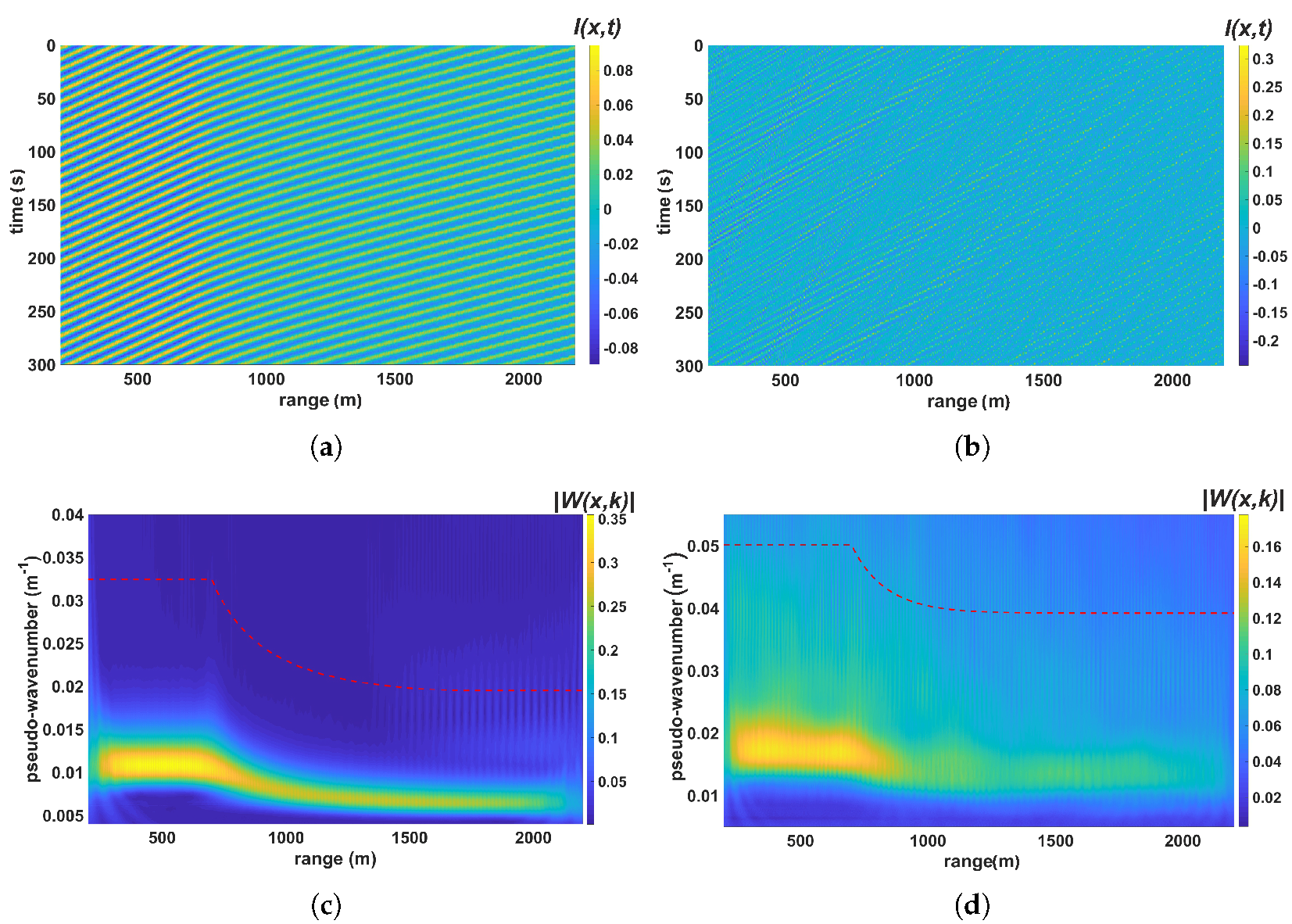
5. Simulation of the Sea Clutter Images and Their Wavelet Analysis

The creation of modeled radar images from original surface elevation maps requires several steps. First, a shadowing mask is applied to define the shadowing modulation: I s h ( x , t ) = ζ ( x , t ) · κ ( x , t ) . The function κ = 1 χ is an indicator of the illuminated (not shadowed) area with χ , as defined in Equation (11). Second, the tilt modulation should be introduced. For this purpose, the surface elevation slope ζ x is required. It can be defined either analytically or with finite differences from Equation (1). The joint tilt and shadowing modulation are calculated as follows:
I t i l t + s h = ( n · u ) , if ( n · u ) > 0 and κ = 1 , 0 , otherwise .
Here, u is the unitary vector starting at point ζ ( x , t ) and pointing to the radar (see Figure 4), ( · ) is the scalar product in a 2D Euclidean space, and n is the external unitary normal vector to the surface point ζ ( x , t ) . It is calculated as n = ρ x × ρ z / | ρ x × ρ z | , where only the first two components of the resulting vector are considered, ρ x = ( 1 , ζ x , 0 ) , and ρ z = ( 0 , 0 , 1 ) .
Third, the speckle noise model presented by Equation (14) is applied using a realization of the random 2D Gaussian noise with zero mean and dispersion n l ( 0 n l < 1 ). For convenience, the noise level is given as a percentage.
It is important to note that all imaging mechanisms are range dependent as they use the local incident angle in their definitions. In coastal probing, this angle changes significantly within the radar footprint. To ensure the requirement of working in the far zone in the modeled sea clutter image, a constant range offset of R 0 = 200 m is added. Finally, the range trend due to the radar equation is added using Equation (10).
To start working with simulated images constructed using the above procedure or a real X-band radar image, the time-averaged range trend first needs to be subtracted using the radar equation. In real radars, the backscattered signal is further amplified, usually with a logarithmic amplifier. This amplification trend should also be treated before applying the inversion procedure. Implementation examples of the described technique for a monochromatic wave and for a JONSWAP spectrum together with their corresponding wavelet spectra are given in Figure 5.

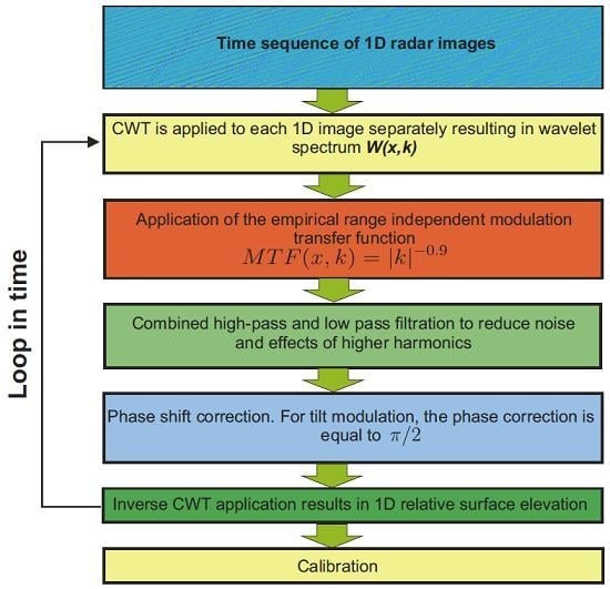
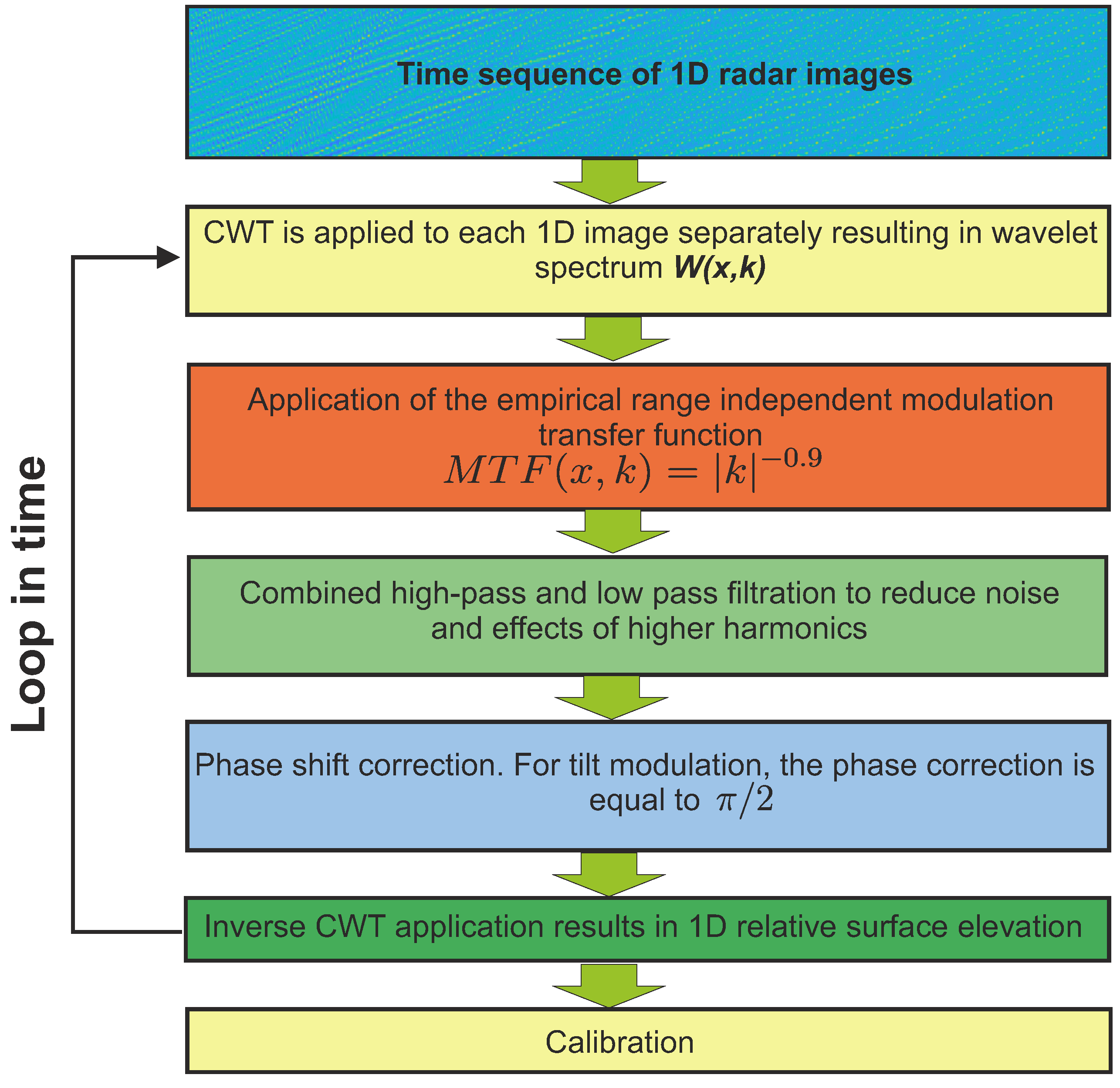
6. Inversion of the Simulated Radar Images into Surface Elevations (Wavelet Analysis)

In this section, a wavelet method for radar image inversion to surface elevation maps is introduced. One of the strengths of the proposed approach is that the procedure is applied to each time instant independently. This allows to the inversion to be performed without information on the dispersion relation. Normally, filters are applied to account for the dispersion relation information. In case of shoaling over a sloping bottom, the dispersion relation can only be defined locally as a function of depth. Here, since it is not possible to account for dispersion relation information in a global image, a higher harmonic filtration is performed in the wave number domain only by means of a special low-pass (LP) filter. In order to avoid the limitations of the conventional method while working with spatially inhomogeneous data, the CWTFT is used as a basis for a new radar image processing method.
The new image inversion method consists of the following procedure (also see the block diagram in Figure 6):
  • Estimation of the CWTFT coefficients of a radar image W [ I ( x , t i ) , ψ ( x ) ] ( x , k ) at a fixed time instance t i and calculation of the correspondent pseudo-wave numbers.
  • Application of the empirical Modulation-Transfer Function (MTF) in a wave number-coordinate domain MTF ( x , k ) = | k | β . The empirical power β is set to 0.9 for all applications. The wavelet-based technique allows the β to vary with the range; nevertheless, a range independent MTF is employed as a first approximation. The details of the MTF’s choice are discussed in Appendix C.
  • Use of combined high-pass (HP) and LP filters F to reduce noise and influence of higher harmonics. The corresponding filter in the wave number-coordinate domain is defined as F ( x , k ) = X { ( x , k ) | k 0 < k < l k p ( x ) , x m i n x x m a x } , where X denotes a characteristic function of a set of points, k 0 is constant in space (0.001 m 1 used in this paper), k p ( x ) is the line of maximum energy in a wavelet spectral domain as a function of space, and l is an empirical constant. Here, the value l = 3 is used for both monochromatic wave and spectrum cases. The filtered wavelet spectrum is further defined as W F [ I ( x , t i ) , ψ ( x ) ] ( x , k ) = W [ I ( x , t i ) , ψ ( x ) ] ( x , k ) · F ( x , k ) .
  • Phase shift correction: As geometrical mechanisms are used, a phase shift equal to π / 2 is applied to every complex spectral wavelet component.
  • Calculation of the inverse CWTFT and calibration: Denoting the ICWTFT as ζ ˘ , the calibrated surface elevation is defined as ζ ˜ = ζ ˘ σ a l l [ ζ ] / σ a l l [ ζ ˘ ] , where σ a l l is the time averaged standard deviation of a 2D array denoted as A in the range defined in Equation (16).
    σ a l l [ A ] = 1 N t i = 1 N t 1 N x 1 j = 1 N x A ( x j , t i ) 1 N x j = 1 N x A ( x j , t i ) 2 1 / 2 .
In order to analyze the obtained results, the absolute error of the reconstruction Δ a ( x , t ) = | ζ ( x , t ) ζ ˜ ( x , t ) | is calculated. Together with Equation (16), some other statistics are useful for the error analysis. To estimate the error on specific time sections, its standard deviation and mean value are introduced by Equations (17) and (19) respectively. To estimate the overall mean value of the error, expression (18) is used, whilst, for a time averaged absolute value as a function of range, Equation (20) is employed.
σ s e c t 0 [ A ] = 1 N x 1 j = 1 N x A ( x j , t 0 ) 1 N x j = 1 N x A ( x j , t 0 ) 2 1 / 2 ,
M a l l [ A ] = 1 N x N t i = 1 N t j = 1 N x A ( x j , t i ) ,
M s e c t 0 [ A ] = 1 N x i = 1 N x A ( x i , t 0 ) ,
M t [ A ] ( x ) = 1 N t i = 1 N t A ( x , t i ) .
The cross-correlation coefficient is defined by the following equation
C s e c t 0 [ A , B ] = 1 ( N x 1 ) σ s e c t 0 [ B ] σ s e c t 0 [ A ] i = 1 N x A ( x i , t 0 ) M s e c t 0 [ A ] B ( x i , t 0 ) M s e c t 0 [ B ] .
In Equations (16)–(21), letters A and B denote 2D arrays of equal sizes, for which the corresponding statistics are calculated. In the cases mentioned hereafter, A and B are substituted with specific notations of the array they are applied to (e.g., ζ , ζ ˘ , ζ ˜ , Δ , or Δ a ). For brevity, the correlation coefficient notation C ζ , ζ ˜ might be used instead of C s e c t 0 [ ζ , ζ ˜ ] when it is clear which cross-section is taken.
In Figure 7 the range–time diagram of the original reconstructed map difference Δ = ζ ( x , t ) ζ ˜ ( x , t ) for the monochromatic wave and the JONSWAP spectrum together with M t [ Δ a ] ( x ) values and the corresponding shadowing probability (refer to the Equation (12)) are given both for the conventional method and for the new one.
From the difference maps, it is clear that the new method shows much better performance in the reconstruction of the surface elevation. Some local extreme values of the corresponding differences for the new method appear only in strongly shadowed troughs.
Since the Fourier transform based CWT is used, the first and last 200 m in the reconstructed image are not taken into account in the estimation of the error statistics (summarized in Table 2) in order to disregard edge effects. A comparison between the original and reconstructed instantaneous surface elevation profiles is presented in Figure 8. The corresponding statistical parameters are given in the last three columns of Table 2, showing a high correlation between the original and reconstructed signals on the section with a comparatively small mean error and dispersion. Unlike the conventional method, the results of the present method demonstrate a very high correlation between the original and reconstructed surface elevations. The speckle noise, which is clearly seen, especially in the shadowed troughs on the cross-section of the corresponding radar images (orange curves in Figure 8a,c), is filtered out in the resulting image due to the use of the corresponding LP filter in the wave number-coordinate domain. The present method also grasps the individual wave heights and crest/trough locations significantly better.

7. Analysis of the Results

In this section, the accuracy of the new wavelet based method is evaluated extensively with respect to various geometric (antenna height), environmental (bathymetry and speckle-noise level), and sea state parameters. The shadowing probability is a function of several parameters, e.g., the incident angle and variation of the surface slopes ε R M S , which are functions of the range (for details refer to Appendix A). For simplification, the mean amount of shadowing is controlled solely using the radar installation height H r . In Figure 9a, the error ( Δ a ( x , t ) ) mean value and its standard deviation averaged over time and space are given using Equations (16) and (18), respectively. They are given as functions of the radar installation height H r both for the entire range–time map and an arbitrarily chosen cross-section. The dependence of the cross-correlation coefficient (Equation (21)) of the original and reconstructed surface elevations is also presented with respect to H r . The results are averaged over the nine bathymetry profiles given in Appendix B and three JONSWAP spectra (for simulation parameters details, refer to Table 1).
In Figure 9a, it can be clearly seen that as the shadowing probability increases (antenna height decreases), the accuracy of the inversion method decreases. This behavior is expected as the shadowed patches contain no backscatter information from the surface elevation for the inversion procedure. The calculated values relate to an averaging over the complete image with respect to H r ; nevertheless, the argument H r does not necessarily relate to the actual antenna height but serves as a measure of shadowing. Parts of the image area can have a local shadowing probability which corresponds to very high antenna installations, and other parts of the image correspond to very low antenna installations. This implies that there is quite a high accuracy level as long as the shadowing probability is low at a certain range.
Figure 9b shows the influence of the speckle noise level on the accuracy of the inversion procedure. As expected, a higher noise percentage reduces the accuracy. Still, typical speckle noise contamination values (≈10%) do not affect the inversion significantly.

8. Conclusions

A new wavelet-based algorithm for the inversion of inhomogeneous radar images was presented. It enables a thorough analysis of shoaling processes, including wave amplitude and length changes, taking the whole image in space as is. The proposed method shows high efficiency in filtering speckle noise and in treating local wave phase shifts due to tilt effects. For the grazing incidence ( H r 20 m), the new method indicates the same level of accuracy for inhomogeneous shoaling conditions as the conventional one in homogeneous sea states (compare [12]). Despite the fact that 1D and 2D cases are compared, the lack of a broader accuracy analysis of the conventional method performance in 1D makes it possible to use this result as reference. As the probability of shadowing decreases ( H r increases), the corresponding accuracy of the new method improves significantly.
The new method addresses the intrinsic limitation of conventional FFT-based methods of accounting for the inhomogeneous conditions common to wave shoaling. In such cases, the conventional method cannot apply the phase shift correctly which can be easily overcome by the localized wavelet-based technique. In this paper, the effect of linear shoaling was taken into account. This kind of process deals with a significant wave number modulation and mild amplitude changes. In cases with strong amplitude modulations, such as in wave grouping and rogue waves, additional investigation of the method performance is needed.
The range resolution used in this paper is finer than that provided by typical nautical radars and ensures a sufficient sampling rate, accounting for wavelength shortening. When working with a typical nautical radar’s range resolution of 4.5–10 m, it is important to limit the analysis to a certain wavelength range, remembering the limitation of 10 sample points per peak wavelength. This can be checked directly with the CWT spectrum analysis.
There are various possible extensions to the described wavelet approach. The new model could be extended to include more advanced adaptive HP and LP filters in the pseudo-wavenumber coordinate domain by choosing the corresponding band-pass in accordance with the spectral width to allow more efficient filtration of the higher harmonics. Without significant changes to the algorithm, the wavelet method could also be extended to 2D spatial cases. Additionally, a localized (coordinate dependent) MTF could be derived to improve the inversion performance in a global nearshore image. It is important to stress that with minor changes to the MTF, the same model could be used for moderate incidences, which are common for airborne and spaceborne radars. In cases where it is impossible to obtain a temporal sequence of the same area (required for the conventional method), the ability of the wavelet method to treat individual spatial images could make it the prominent approach for moving platforms.

Author Contributions

P.C., under the supervision of Y.T., proposed the inversion technique, performed the program realization of the synthetic radar images together with the inversion block and error analysis, wrote the manuscript Section 1, Section 3, Section 4, Section 5, Section 6, Section 7 and Section 8, Appendix A, Appendix B, Appendix C and Appendix D. T.V. prepared the rough sea surface realization code for the shoaling conditions and wrote Section 2.

Funding

The work was supported by the Israeli Ministry of Science and Technology (grant No. 3-12473) and Federal Ministry of Education and Research (BMBF), Germany (grant No. 3-15249).

Acknowledgments

The authors would like to thank Sara Nauri and Anna Chernyshova from the School of mechanical engineering, Tel-Aviv University for inspiration and significant help in improving the manuscript.

Conflicts of Interest

The authors declare no conflict of interest.

Abbreviations

The following abbreviations are used in this manuscript:
CWTContinuous Wavelet Transform
CWTFTContinuous Wavelet Transform with Fourier Transform
ICWTFTInverse Continuous Wavelet Transform with Fourier Transform
FFTFast Fourier Transform
MTFModulation Transfer Function
JONSWAPJOint North Sea WAve Project
SARSynthetic Aperture Radar
LPLow-Pass (filter)
HPHigh-Pass (filter)

Appendix A. The Shadowing Probability, Accounting for Linear Shoaling Conditions

For typical probability density functions of heights and slopes of monochromatic waves or with normal distributions, rather compact analytical expressions for shadowing probability have been presented, e.g., in [30,31]. In the case of linear shoaling, the corresponding expressions can be modified as follows. The probability of shadowing for a random surface with a characteristic (RMS) slope ε R M S 2 ( x ) = ( d ζ / d x ) 2 is
S ( H r , x , ε R M S ) = Λ ( b ) + 1 / 2 erfc ( b / 2 ) Λ ( b ) + 1 ,
where Λ g ( b ) = 2 π b 1 e b 2 / 2 erfc ( b / 2 ) 2 for locally Gaussian distributions and Λ m ( b ) = 1 π 2 / b 1 arccos ( b / 2 ) for monochromatic wave distributions. In previous expressions, b = H r / ( x ε R M S ) , erfc ( x ) = x e t 2 d t . The corresponding ε R M S ( x ) can be calculated as
ε R M S g ( x ) = 2 H s ( x ) k p ( x ) / 4 π , ε R M S m ( x ) = a ( x ) k ( x ) / π .
Here, the significant wave height evolution can be defined as
H s ( x ) = 4 0 S ( ω ) C g ( k ( ω , h ( 0 ) ) , h ( 0 ) ) C g ( k ( ω , h ( x ) ) , h ( x ) ) d ω 1 / 2 .
The peak wave number k p ( x ) as a function of range is obtained as the root of the dispersion relation shown in Equation (2) with the frequency value of ω p = 2 π / T p , assuming a weak dependence of ω p on the range, which is reasonable for linear shoaling cases. The amplitude evolution a ( x ) is defined by Equation (5).

Appendix B. Utilization of the Conventional Method for the Radar Image Sequences Inversion in 1D Case

In this paper, the conventional method is adopted and utilized for a 1D case in accordance with its original introduction in [9] for the inversion of 2D spatial radar image sequences to surface elevation maps. A number of simulations, including both monochromatic wave and JONSWAP spectrum cases (with and without shoaling) were tested on a set of simulated 1D radar image sequences. Generally, the results revealed that the conventional method produced much poorer results in 1D than in 2D cases, due to spectral leakage effects and a finite (coarse) resolution in the spectral domain. Sometimes, even for the simplest case of a propagating monochromatic wave, the inverse wave had a frequency deviation equal to the frequency step Δ ω in Fourier space and necessarily resulted in a discrepancy in comparison with the original image. For the 2D cases, this issue seemed to matter less due to availability of information in the lateral wave number, which might compensate the frequency deviation effect. The above confirms and expands on previous considerations on conventional methods presented in literature (e.g., the paper [13] mentioned in the introduction as a part of the literature review, also [32,33]).
The addition of linear shoaling revealed other limitations of the conventional method, as it did not satisfy the assumption of signal’s spatial homogeneity and periodicity. Without the advantage of the localization in space, which was performed in the wavelet analysis case, the conventional method’s FFT will put the signals coming from deeper and shallower waters on the same frequency line, but with different wave numbers, which will lead to the formation of a two-pronged signal in the spectral domain following two dispersion relation curves—one for deep waters and another for shallow waters (see black and red curves in the Figure A1). This requires the use of quite a wide dispersion relation shell to fit all of the signals inside. Any type of windowing will not solve the problem due to the fact that there regularly exists an area with a significant wave number gradient in transition from intermediate to shallow waters (see, e.g., the area limited by 600 < x < 1000 in the range of the wavelet spectrum for the JONSWAP spectrum case from Figure 3b), which will demonstrate the same effect even on a comparatively small window.
Since the utilization of the conventional method in 1D (non-homogeneous) case has not previously been described in the literature, the algorithm used in the paper is given below.
  • Estimation of the complex 2D Fourier spectrum F [ I ( x , t ) ] ( k , ω ) of a 1D radar image sequence. To mitigate the aliasing effect, the area of the negative frequencies ω < 0 is cut and pasted above the Nyquist frequency.
  • Application of the dispersion relation shell filter in order to separate the signals of wave modulations from the higher harmonics. The resulting filtered signal contains the following set of harmonics { F [ I ] ( k , ω ) : ω k · U g k tanh ( k h mean ) Δ f / 2 } , where h mean is the arithmetic average between the minimal and the maximal depth over the image area, U is the uniform current, and Δ f is the width of the filter.
  • Application of the empirical Modulation-Transfer Function to the spectral amplitudes MTF = | k | 1 . 2 [9].
  • HP filtration, which passes all the components higher than a certain limiting wave number k t h and corresponding frequency ω t h . According to [34] it is plausible to take ω t h = 0 . 19 rad/s. The corresponding k t h is calculated using the dispersion relation accounting for the minimal water depth ( h m i n ).
  • Phase shift correction: As geometrical mechanisms are used, a phase shift equal to π / 2 should be applied to every complex spectral component. The constant phase shift is applicable only in case of homogenous and periodic signals. In cases of linear shoaling, when the phase of the original signal is defined as in Equation (1), this step does not give the desired result and hence becomes optional.
  • Calculation of the inverse FFT, taking the real part of the resulting array and calibration. The calibration is conducted using the same approach as described in the new method.
The results of the conventional method application to the inhomogeneous radar images, both for the monochromatic wave and the JONSWAP spectrum case, and their comparison with the new method are given in Figure 7a,b,e,g and Figure 8b,d. For the monochromatic and the JONSWAP spectrum cases, the same dispersion relation filter parameters were applied. For simplicity, the wave–current interactions were neglected, as they do not affect the new method (it works in the wave number-coordinate wavelet domain and does not rely on the dispersion relation filter). For the conventional method, the consideration of the current adds just one step to fit into the wavenumber-frequency domain.
Figure A1. Example of the 2D ( k ω ) Fourier spectrum for the utilization of the conventional method in 1D case after stages 1 and 2 were applied to the radar image of the JONSWAP spectrum case from Figure 5b. The wind wave signal is inscribed in the broad dispersion relation filter ( Δ f / 2 = U 0 = 0 . 15 rad/s) based on the mean depth h mean = 35 m. It is clear that the signal from the waves forms a two-pronged pattern following two dispersion relations, one for deeper waters ( h min = 60 m), another for shallower waters ( h max = 10 m). The manifestation of higher harmonics and group line is also evident.
Remotesensing 10 01919 g0a1

Appendix C. Modulation-Transfer Function Discussion

The choice of the MTF is a crucial aspect of any radar image inversion technique, and a debatable one. Historically, several approaches have been used. The MTF was first introduced and evaluated in [9]. The power β was found there to be 1.2 by fitting the measured spectra to the omnidirectional spectra of radar images derived using a dispersion relation shell filter in the wave number-frequency domain. In that paper, for different sea state conditions arbitrarily selected from 3 days of measurement ( 1 . 9 < H s < 4 . 3 m), the power of MTF varied from 0.97 to 1.37, and its mean value, 1.2, was selected. This value is commonly used in conventional methods. In [19], a piecewise constant model for the MTF power was proposed in order to attain the best fit with the power law of the weak turbulence theory, whereas in [35], a similar fitting was done in the spectral domain under logarithmic coordinates using a parabolic model of the MTF (the original MTF corresponds to the linear model in logarithmic coordinates). These three examples show that, currently, there is no universal agreement on either the value of the power β or on the shape of the MTF to be used. It should also be noted that all the MTFs are fitted in the spectral domain due to the fact that in point measurements there is no option to compare the results of the original and reconstructed time series directly at all spatial points.
The same power-shaped MTF model used in [9] is used in the new proposed wavelet based method with a fundamental difference. Whilst the conventional method operates in the wave number-frequency domain, the wavelet based one works in a pseudo-wave number coordinate domain; hence, the pseudo-wavenumber is the one employed in the MTF. In a set of numerical experiments with different sea-state and bathymetry conditions with a fixed probing geometry, the power β varied in a range from 0.5 to 1.5 with a step of 0.1. Using the minimization of the mean error and variance between the original and reconstructed profiles as criteria resulted in a value β of 0.9. This value of β was then used as a constant for all numerical simulations shown in this paper.
Another important aspect of the MTF, which is less discussed in the literature, is the phase shift correction. It was shown in [11] that, for a purely monochromatic wave and tilt modulation, the corresponding MTF is an imaginary value, providing a π / 2 phase shift in the spectral domain. The complication starts when the signal is wave number modulated (e.g., in the shoaling conditions regarded in this paper). In fact, in such cases, the conventional method is unable to correctly apply the corresponding phase shift, while the localized wavelet based technique easily does this (see Figure 7 and Figure 8). This seems to be one of the main reason why the conventional method fails to analyze the shoaling wave image globally.

Appendix D. Bathymetry Profiles

The nine bathymetry profiles used in the numerical simulations are presented below.
h 1 ( x ) = 10 200 x 700 , 60 1700 < x 2200 , x 20 25 700 < x 1700 ;
h 2 ( x ) = 10 200 x 550 , 60 1800 < x 2200 , x 25 12 550 < x 1800 ;
h 3 ( x ) = 10 200 x 333 , 60 2000 < x 2200 , 10 ( 5 x + 2 ) 1667 333 < x 2000 ;
h 4 ( x ) = 30 200 x 450 , 60 1950 < x 2200 , x 50 + 21 450 < x 1950 ;
h 5 ( x ) = 45 200 x 450 , 60 1950 < x 2200 , x + 4050 100 450 < x 1950 ;
h 6 ( x ) = 10 200 x 700 , 60 1700 < x 2200 , 3 x 50 42 1200 < x 1700 , x 25 18 700 < x 1200 ;
h 7 ( x ) = 10 200 x 700 , 60 1700 < x 2200 , 4 x 25 212 1450 < x 1700 , x + 50 75 700 < x 1450 ;
h 8 ( x ) = 10 200 x 700 , 60 1700 < x 1900 2000 < x 2200 , 820 2 x 5 1900 < x 1950 , 2 x 5 740 1950 < x 2000 , x 20 25 700 < x 1700 ;
h 9 ( x ) = 10 200 x 700 , 60 1450 < x 2200 , 403 . 341 0 . 33334 x 1100 < x 1150 , 0 . 46666 x 516 . 659 1150 < x 1200 , 0 . 066668 x 36 . 6686 1200 < x 1450 , 0 . 0666675 x 36 . 6673 700 < x 1100 .

References

  1. Borge, J.C.N.; Reichert, K.; Dittmer, J. Use of nautical radar as a wave monitoring instrument. Coast. Eng. 1999, 37, 331–342. [Google Scholar] [CrossRef]
  2. Nieto-Borge, J.; Hessner, K.; Jarabo-Amores, P.; de La Mata-Moya, D. Signal-to-noise ratio analysis to estimate ocean wave heights from X-band marine radar image time series. IET Radar Sonar Navig. 2008, 2, 35–41. [Google Scholar] [CrossRef]
  3. Senet, C.M.; Seemann, J.; Flampouris, S.; Ziemer, F. Determination of bathymetric and current maps by the method DiSC based on the analysis of nautical X-band radar image sequences of the sea surface (November 2007). IEEE Trans. Geosci. Remote Sens. 2008, 46, 2267–2279. [Google Scholar] [CrossRef]
  4. Serafino, F.; Lugni, C.; Nieto Borge, J.C.; Zamparelli, V.; Soldovieri, F. Bathymetry determination via X-band radar data: A new strategy and numerical results. Sensors 2010, 10, 6522–6534. [Google Scholar] [CrossRef] [PubMed] [Green Version]
  5. Lebedev, I.; Tomczak, M. Rainfall measurements with navigational radar. J. Geophys. Res. Ocean. 1999, 104, 13697–13708. [Google Scholar] [CrossRef] [Green Version]
  6. Dankert, H.; Horstmann, J.; Rosenthal, W. Ocean wind fields retrieved from radar-image sequences. J. Geophys. Res. 2003, 108. [Google Scholar] [CrossRef] [Green Version]
  7. Kanevsky, M.B. Radar Imaging of the Ocean Waves; Elsevier: Amsterdam, The Netherlands, 2008. [Google Scholar]
  8. Valenzuela, G.R. Theories for the interaction of electromagnetic and oceanic waves—A review. Bound.-Layer Meteorol. 1978, 13, 61–85. [Google Scholar] [CrossRef]
  9. Borge, J.C.N.; Rodríguez, G.R.; Hessner, K.; González, P.I. Inversion of marine radar images for surface wave analysis. J. Atmos. Ocean. Technol. 2004, 21, 1291–1300. [Google Scholar] [CrossRef]
  10. Salcedo-Sanz, S.; Borge, J.N.; Carro-Calvo, L.; Cuadra, L.; Hessner, K.; Alexandre, E. Significant wave height estimation using SVR algorithms and shadowing information from simulated and real measured X-band radar images of the sea surface. Ocean Eng. 2015, 101, 244–253. [Google Scholar] [CrossRef]
  11. Alpers, W.; Hasselmann, K. The two-frequency microwave technique for measuring ocean-wave spectra from an airplane or satellite. Bound.-Layer Meteorol. 1978, 13, 215–230. [Google Scholar] [CrossRef]
  12. Chernyshov, P.; Ivonin, D.; Khalikov, Z.; Myslenkov, S. Accuracy analysis of individual waves retrieval from X-band radar brightness images by implementation of stochastic modeling of rough sea surface. Sovremmennie Probl. Distansionnogo Zondirovaniya Zemli Iz Kosmosa 2016, 13, 68–78. (In Russian) [Google Scholar] [CrossRef]
  13. Wei, Y.; Zhang, J.K.; Lu, Z. A Novel Successive Cancellation Method to Retrieve Sea Wave Components from Spatio-Temporal Remote Sensing Image Sequences. Remote Sens. 2016, 8, 607. [Google Scholar] [CrossRef]
  14. Daubechies, I. The wavelet transform, time-frequency localization and signal analysis. IEEE Trans. Inf. Theory 1990, 36, 961–1005. [Google Scholar] [CrossRef]
  15. Wu, L.C.; Chuang, L.Z.H.; Doong, D.J.; Kao, C.C. Ocean remotely sensed image analysis using two-dimensional continuous wavelet transforms. Int. J. Remote Sens. 2011, 32, 8779–8798. [Google Scholar] [CrossRef]
  16. An, J.; Huang, W.; Gill, E.W. A self-adaptive wavelet-based algorithm for wave measurement using nautical radar. IEEE Trans. Geosci. Remote Sens. 2015, 53, 567–577. [Google Scholar] [CrossRef]
  17. Chuang, L.Z.H.; Wu, L.C.; Doong, D.J.; Kao, C.C. Two-dimensional continuous wavelet transform of simulated spatial images of waves on a slowly varying topography. Ocean Eng. 2008, 35, 1039–1051. [Google Scholar] [CrossRef]
  18. Doong, D.J.; Wu, L.C.; Kao, C.C.; Chuang, H.; Zsu, L. Wavelet spectrum extracted from coastal marine radar images. In Proceedings of the The Thirteenth International Offshore and Polar Engineering Conference, Honolulu, HI, USA, 25–30 May 2003. [Google Scholar]
  19. Ludeno, G.; Brandini, C.; Lugni, C.; Arturi, D.; Natale, A.; Soldovieri, F.; Gozzini, B.; Serafino, F. Remocean system for the detection of the reflected waves from the costa concordia ship wreck. IEEE J. Sel. Top. Appl. Earth Obs. Remote Sens. 2014, 7, 3011–3018. [Google Scholar] [CrossRef]
  20. Dean, R.G.; Dalrymple, R.A. Water Wave Mechanics for Engineers and Scientists; World Scientific Publishing Co Inc.: Singapore, 1991; Volume 2. [Google Scholar]
  21. Agnon, Y.; Sheremet, A.; Gonsalves, J.; Stiassnie, M. Nonlinear evolution of a unidirectional shoaling wave field. Coast. Eng. 1993, 20, 29–58. [Google Scholar] [CrossRef]
  22. Hasselmann, K.; Barnett, T.; Bouws, E.; Carlson, H.; Cartwright, D.; Enke, K.; Ewing, J.; Gienapp, H.; Hasselmann, D.; Kruseman, P.; et al. Measurements of Wind-Wave Growth and Swell Decay During the Joint North Sea Wave Project (JONSWAP); Technical Report; Deutches Hydrographisches Institut: Hamburg, Germany, 1973. [Google Scholar]
  23. Daubechies, I. Ten Lectures on Wavelets; SIAM: Philadelphia, PA, USA, 1992. [Google Scholar]
  24. Alpers, W.R.; Ross, D.B.; Rufenach, C.L. On the detectability of ocean surface waves by real and synthetic aperture radar. J. Geophys. Res. Ocean. 1981, 86, 6481–6498. [Google Scholar] [CrossRef]
  25. Skolnik, M.I. Radar Handbook; McGraw-Hill Book Co.: New York, NY, USA, 1970. [Google Scholar]
  26. Plant, W.J.; Farquharson, G. Wave shadowing and modulation of microwave backscatter from the ocean. J. Geophys. Res. Ocean. 2012, 117, 1–14. [Google Scholar] [CrossRef]
  27. Gangeskar, R. An algorithm for estimation of wave height from shadowing in X-band radar sea surface images. IEEE Trans. Geosci. Remote Sens. 2014, 52, 3373–3381. [Google Scholar] [CrossRef]
  28. Liu, X.; Huang, W.; Gill, E.W. Comparison of Wave Height Measurement Algorithms for Ship-Borne X-Band Nautical Radar. Canadian J. Remote Sens. 2016, 42, 343–353. [Google Scholar] [CrossRef]
  29. Forouzanfar, M.; Moghaddam, H.A.; Dehghani, M. Speckle reduction in medical ultrasound images using a new multiscale bivariate Bayesian MMSE-based method. In Proceedings of the IEEE 15th Signal Processing and Communications Applications, Eskisehir, Turkey, 11–13 June 2007; pp. 1–4. [Google Scholar]
  30. Smith, B. Geometrical shadowing of a random rough surface. IEEE Trans. Antennas Propag. 1967, 15, 668–671. [Google Scholar] [CrossRef]
  31. Bass, F.; Fuks, I. Wave Scattering from Statistically Rough Surfaces: International Series in Natural Philosophy; Elsevier: Amsterdam, The Netherlands, 2013; Volume 93. [Google Scholar]
  32. Naaijen, P.; Blondel-Couprie, E. Reconstruction and Prediction of Short-Crested Seas Based on the Application of a 3D-FFT on Synthetic Waves. Part 1: Reconstruction. In Proceedings of the ASME 2012 31st International Conference on Ocean, Offshore and Arctic Engineering, Rio de Janeiro, Brazil, 1–6 July 2012; pp. 43–53. [Google Scholar]
  33. Blondel-Couprie, E.; Naaijen, P. Reconstruction and Prediction of Short-Crested Seas Based on the Application of a 3D-FFT on Synthetic Waves. Part 2: Prediction. In Proceedings of the ASME 2012 31st International Conference on Ocean, Offshore and Arctic Engineering, Rio de Janeiro, Brazil, 1–6 July 2012; pp. 55–70. [Google Scholar]
  34. Nieto Borge, J.C.; Guedes Soares, C. Analysis of directional wave fields using X-band navigation radar. Coast. Eng. 2000, 40, 375–391. [Google Scholar] [CrossRef]
  35. Chen, Z.; Zhang, B.; He, Y.; Qiu, Z.; Perrie, W. A new modulation transfer function for ocean wave spectra retrieval from X-band marine radar imagery. Chin. J. Oceanol. Limnol. 2015, 33, 1132–1141. [Google Scholar] [CrossRef]
Figure 1. (a) Surface elevation ζ ( x , t ) range-time diagram for the monochromatic wave shoaling case ( f = 0 . 1 Hz, a 0 = 1 m); (b) ζ ( x , t ) for the JONSWAP spectrum case ( f p = 0 . 14 Hz, H s 0 = 1 . 76 m); (c) cross section ζ ( x , 0 ) corresponding to panel (a), where the wave height is enhanced by factor of 3.5 (solid blue line), bathymetry profile according to Equation (A3) (dashed blue line), and corresponding dimensionless wave number k h (solid orange line); (d) the same as (c) for the JONSWAP spectrum case of panel (b). The values of k h ( k p h ) correspond to intermediate-shallow water depth conditions. The time-space crest slopes change in diagrams (a,b) after entering shallow waters, which corresponds to changes in their celerity.
Remotesensing 10 01919 g001
Figure 2. (a) Evolution of the theoretical wave amplitude in space in accordance with expression (5); (b) evolution of the significant wave height (see Equation (A2)) (JONSWAP spectrum case). Both cases are given for the bathymetry h 1 ( x ) , defined in Equation (A3).
Remotesensing 10 01919 g002
Figure 3. (a) Time-averaged CWTFT (Continuous Wavelet Transform with Fourier Transform) of the monochromatic wave shoaling signal from Figure 1a (with Morlet mother wavelet). The color bar represents the absolute values of the wavelet coefficient which were obtained by averaging 150 successive time samples of the spatial surface elevation; (b) the same for the JONSWAP spectrum case from Figure 1b.
Remotesensing 10 01919 g003
Figure 4. Probing geometry scheme including the illustration of shadowing and tilt modulation as a scalar product of the unitary external normal vector n and the unitary vector pointing to the radar antenna u .
Remotesensing 10 01919 g004
Figure 5. (a) Range-time diagram of the detrended radar image intensity for the monochromatic wave case given in Figure 1a (noise level n l = 10 % , radar height H r = 50 m); (b) the same as panel (a) for the JONSWAP spectrum case given in Figure 1b. The intensities are presented in relative values. Negative values in the intensities appear as a result of image range detrending after the radar equation application. (c,d) Corresponding averaged wavelet spectra of the radar images (a,b) respectively. The red dashed lines mark the low-pass (LP) filter boundary. For the monochromatic wave case in the wavelet spectrum (c), the second harmonic manifestation due to the imaging mechanisms is evident in the stripe 1300 x 2200 m.
Remotesensing 10 01919 g005
Figure 6. Block diagram of the new wavelet-based reconstruction algorithm.
Remotesensing 10 01919 g006
Figure 7. Range–time diagram of the differences between the original and reconstructed images ( Δ ) for the monochromatic wave case (a) with the conventional method and (c) with the new CWTFT-based method; (e) range dependence of the time-averaged absolute error M t [ Δ a ] ( x ) for both methods, and (f) corresponding shadowing probability. (b,d,g,h). The same is shown for the JONSWAP spectrum case. The algorithm for the utilization of the conventional method in 1D case is given in Appendix B.
Remotesensing 10 01919 g007
Figure 8. (a) Comparison of the relative fluctuations of the initial surface elevation and the detrended radar image cross-section for the monochromatic wave case. A π / 2 phase shift, resulting in a one-quarter local wavelength shift in physical space is evident. (b) Comparison between ζ and ζ ˜ for the conventional method and the new CWTFT based method on the same section. The statistical parameters of the comparison are summarized in Table 2 in the last three columns. (c,d) The same is shown for the JONSWAP spectrum case.
Remotesensing 10 01919 g008
Figure 9. (a) Main statistical parameters of the absolute error Δ a with respect to the corresponding shadowing probability (represented by the radar installation height H r ) are summarized as percentages of the significant wave height. The results are additionally averaged over the nine bathymetry profiles and three JONSWAP spectra. (b) The same is shown for the noise level dependence. The radar installation height was 230 m (almost no shadowing conditions) for this set of experiments.
Remotesensing 10 01919 g009aRemotesensing 10 01919 g009b
Table 1. JONSWAP (JOint North Sea WAve Project) spectrum parameters used for surface modeling in the paper.
ParameterValue
fetch (F)500 (km)
wind speed (U)3.2, 9.2, 15.7 (m/s)
peak period ( T p )7, 10, 12 s
initial significant wave height ( H s 0 )1.76, 4.53, 7.33 (m)
time step ( Δ t )2 (s)
spatial step ( Δ x )2 m
spectral resolution ( Δ ω )0.031 (rad/s)
number of harmonics (N)100
number of time samples ( N t )151
number of range samples ( N x )1001
Table 2. Absolute error Δ a statistics for the new CWTFT-based method for the monochromatic wave and JONSWAP spectrum examples given in Figure 1, Figure 2, Figure 3, Figure 4 and Figure 5, Figure 7 and Figure 8. Here mean P s h = M a l l [ χ ] , where χ ( x , t ) is the shadowing mask (see Equation (11)), and the other columns to the right side are defined by Equations (16)–(19) and (21) respectively.
Case H r (m)Mean P sh ( % ) M all [ Δ a ] (m) σ all [ Δ a ] (m) M sec t 0 [ Δ a ] (m) σ sec t 0 [ Δ a ] (m) C ζ , ζ ˜
monochromatic wave50160.0670.0510.0710.0630.991
spectrum50390.1640.1470.1690.1420.872

