Flood Mapping in a Complex Environment Using Bistatic TanDEM-X/TerraSAR-X InSAR Coherence

 ,
,  and
and 
Abstract
1. Introduction
2. Study Area and Dataset
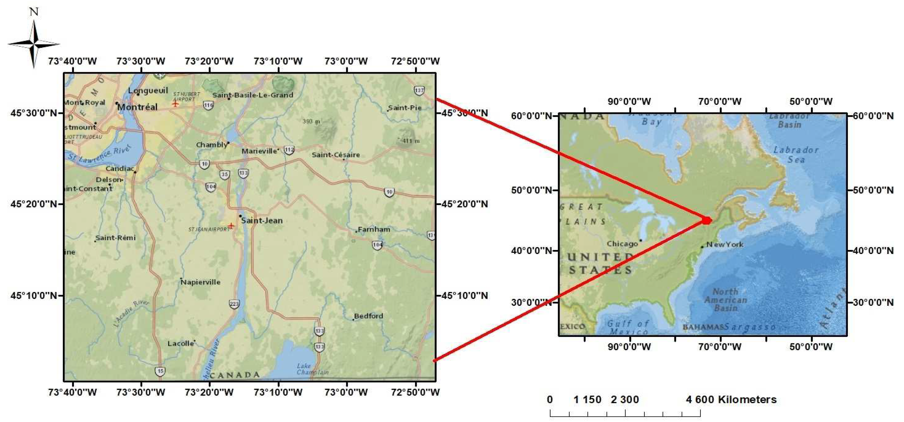
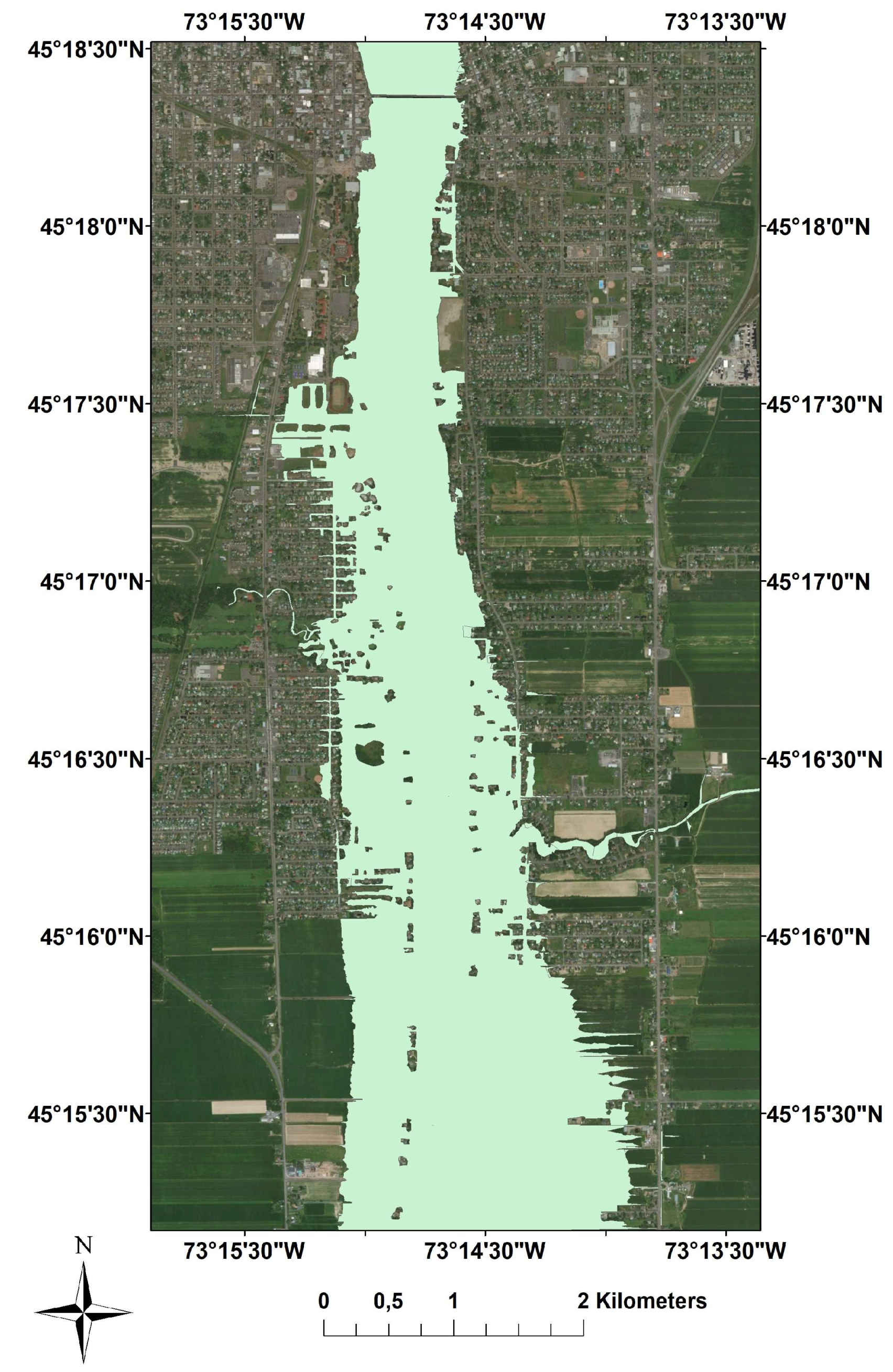
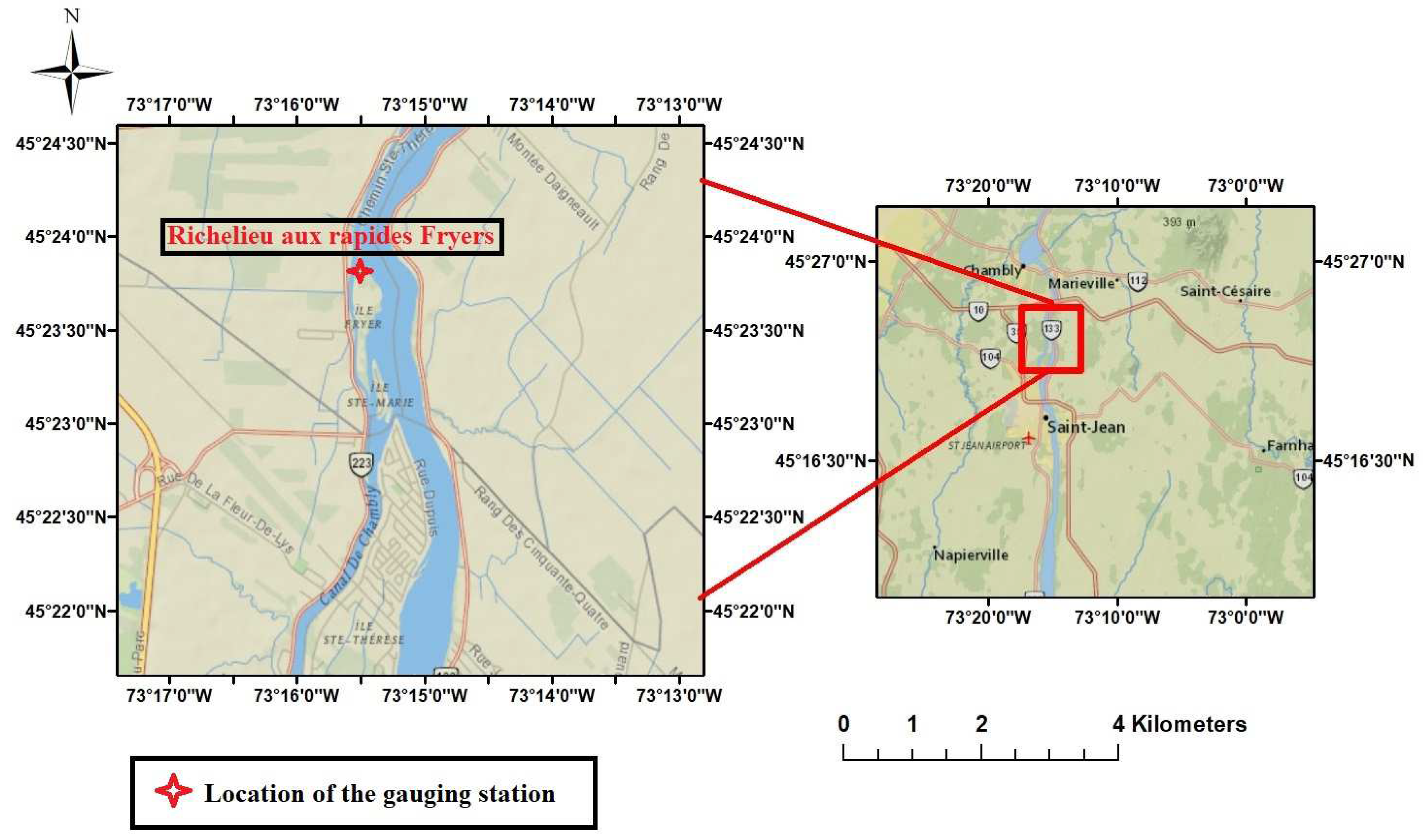
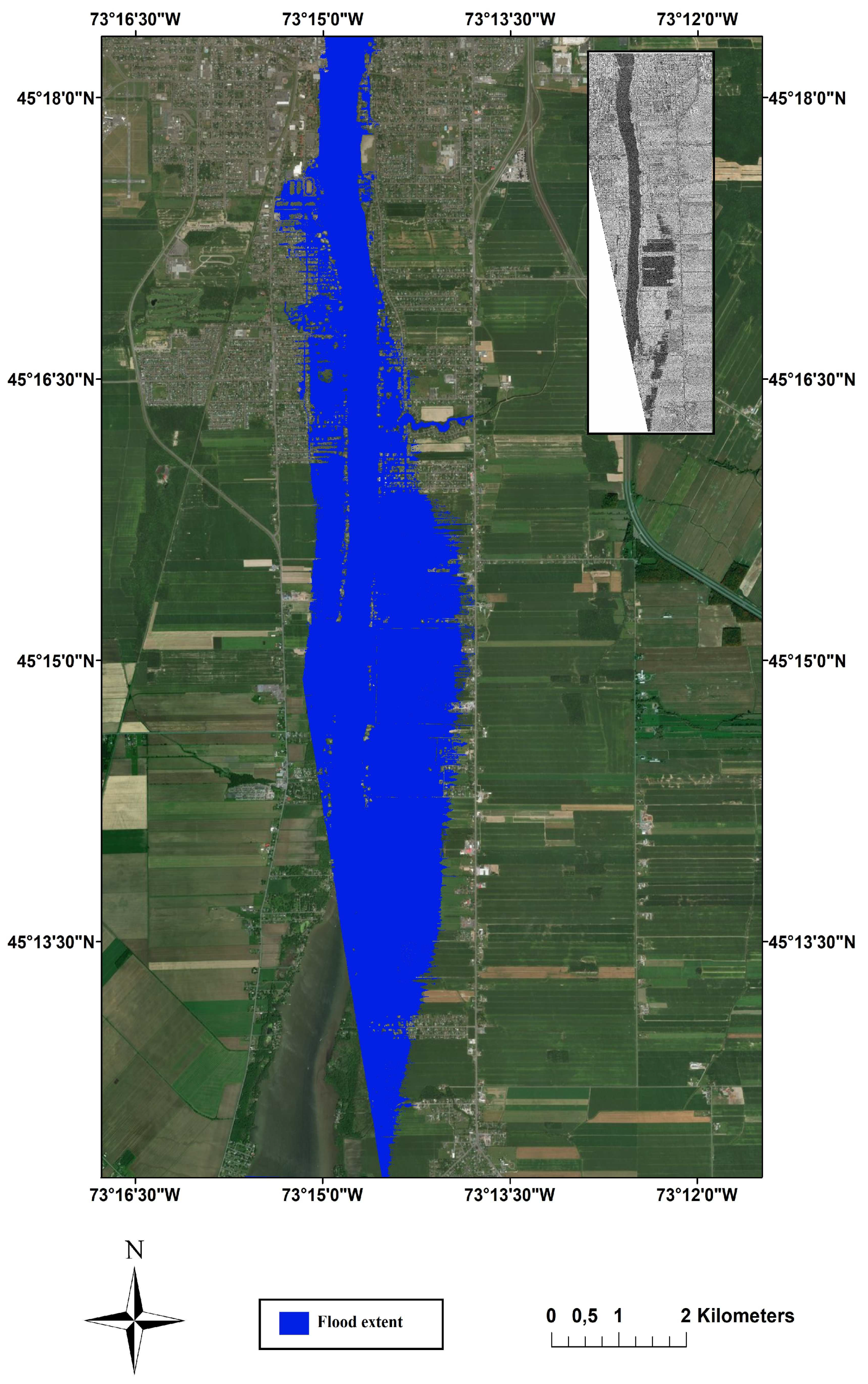
2.1. Study Area
2.2. Available Data Set
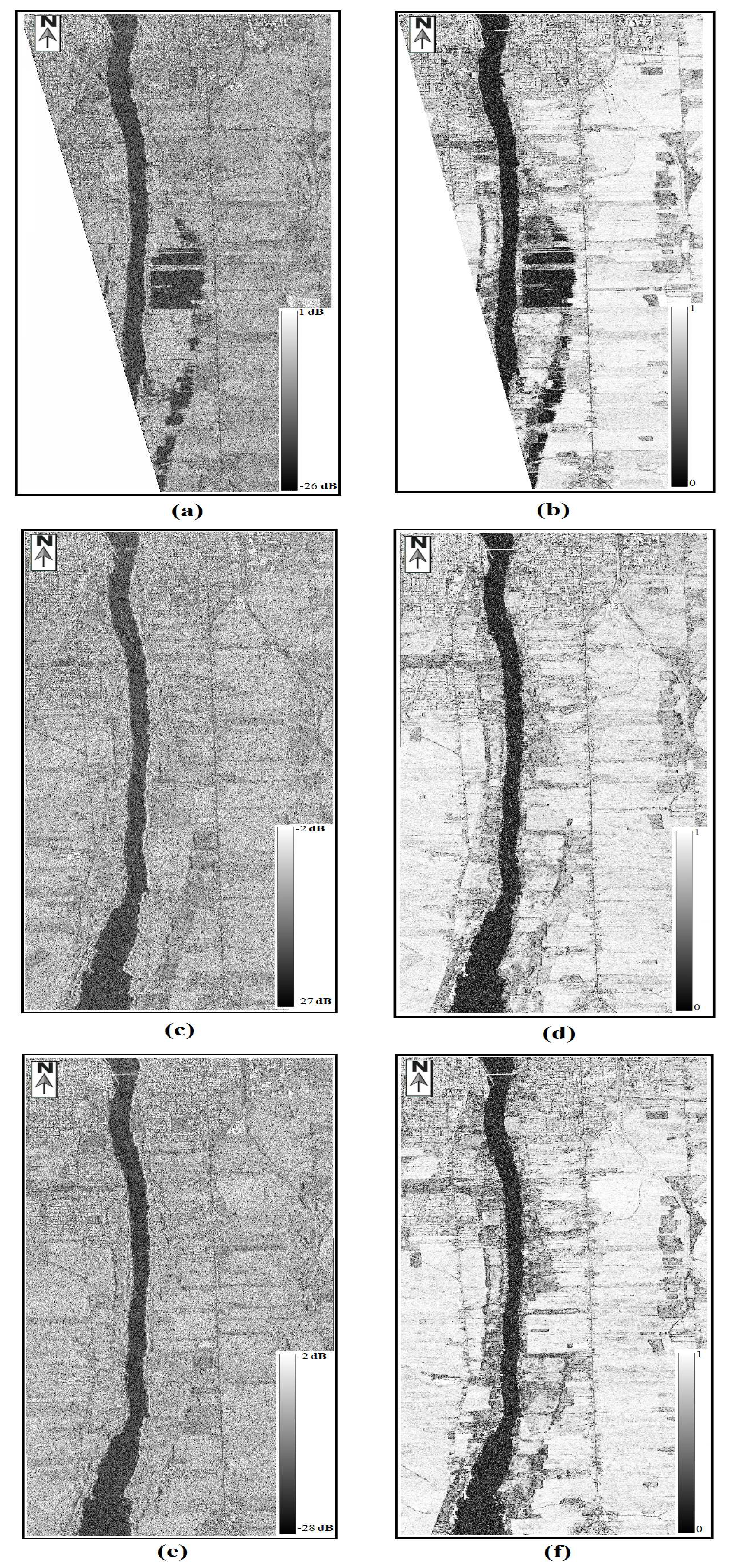
2.2.1. Synthetic Aperture RADAR Data
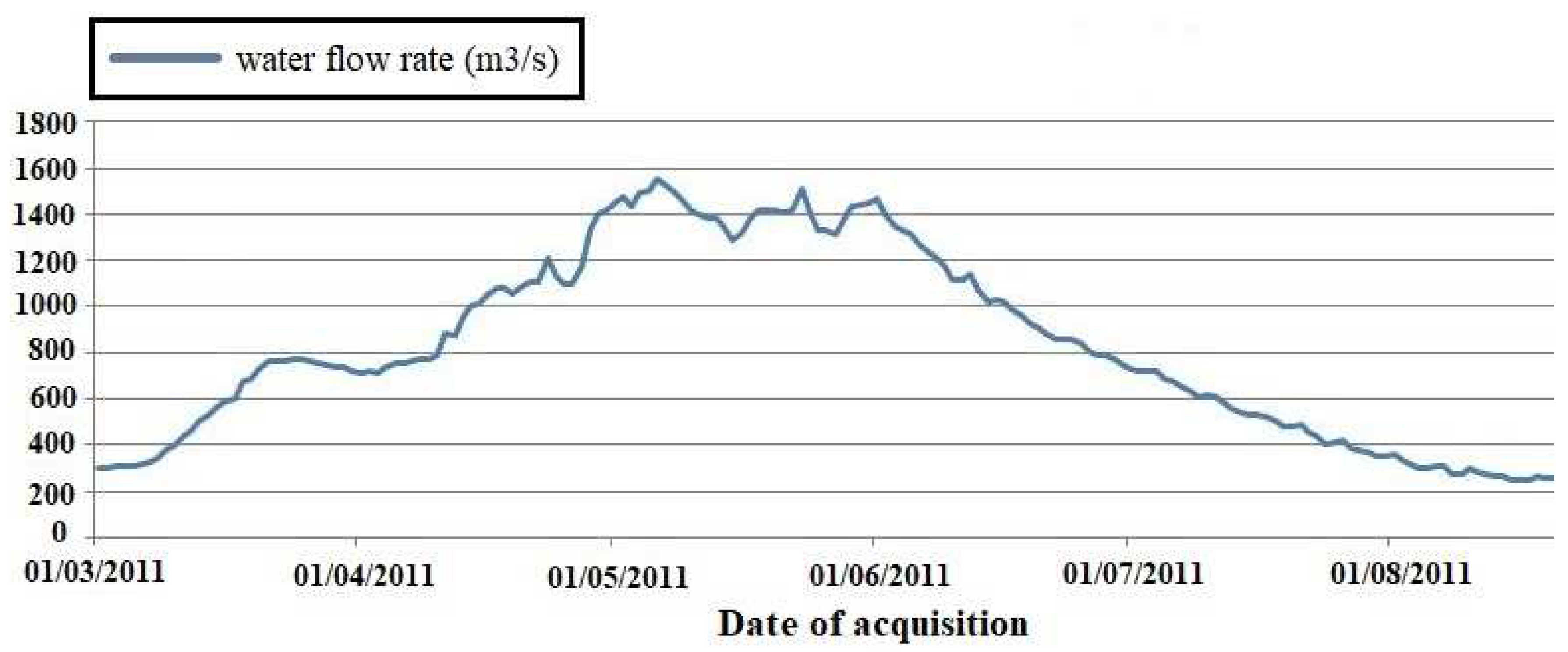
2.2.2. Topographic and Hydrometric Data
3. Data Analysis
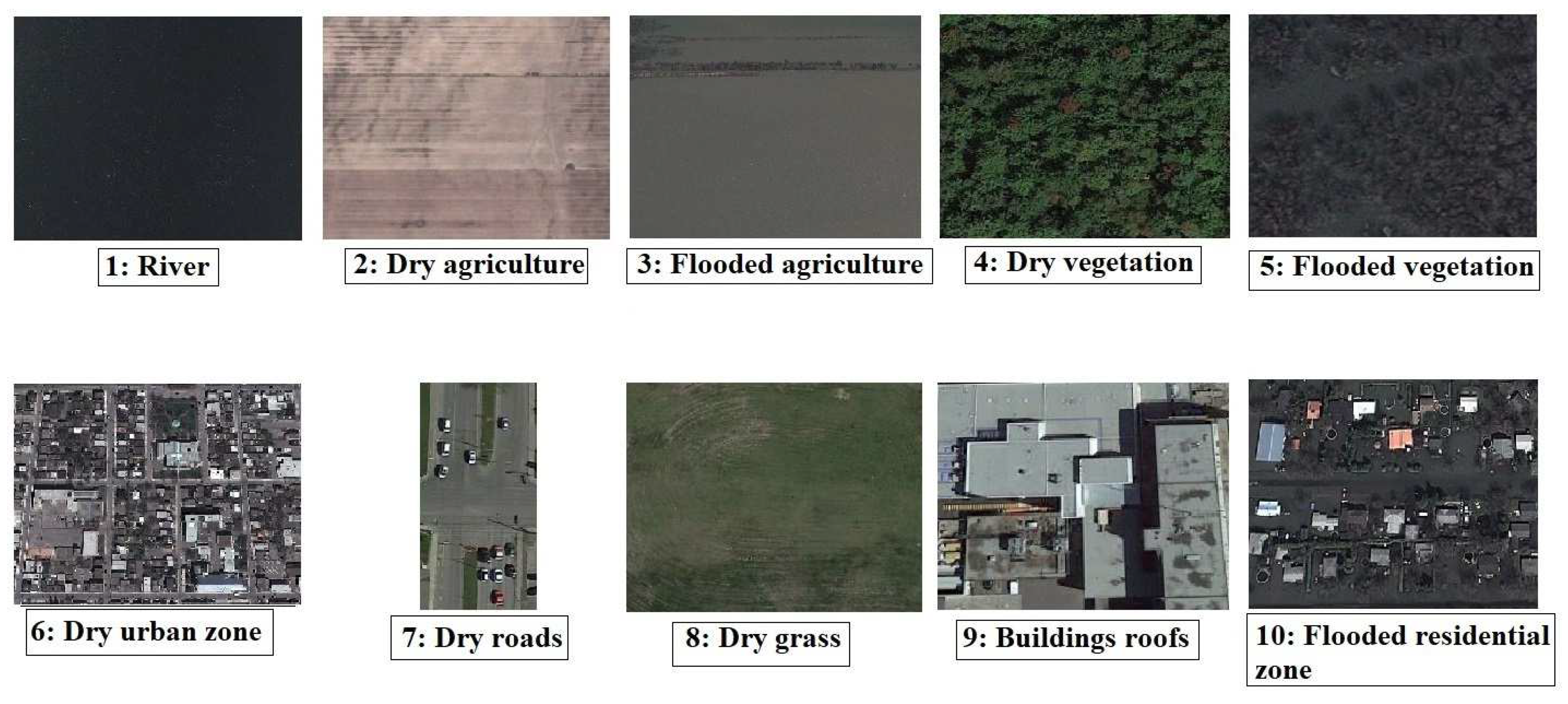
- River: represents different parts of the Richelieu River stream.
- Dry agriculture: represents agricultural zones that remained dry and not affected by the flooding.
- Flooded agriculture: represents the agricultural zones in the river floodplain that were submerged.
- Dry vegetation: represents mainly forest zones that remained dry and not affected by the flooding.
- Flooded vegetation: represents mainly forest zones that were affected by the presence of water during the flood.
- Dry urban zone: represents the urban zone of Saint-Jean-sur-Richelieu city with a dense building topology.
- Dry roads: represents the roads that were not affected by the flooding.
- Dry grass: mainly represents grass (e.g., in public parks or house gardens) that was not affected by flood water.
- Building roofs: represents only the roofs of houses and buildings.
- Flooded residential: represents the residential areas lying in the river floodplain that were identified as flooded during the event. We can notice that the building structure within this ROI is very different when compared to the Dry Urban ROI as the buildings here are mainly sparsely distributed houses.
4. Random Forest Classification Approach
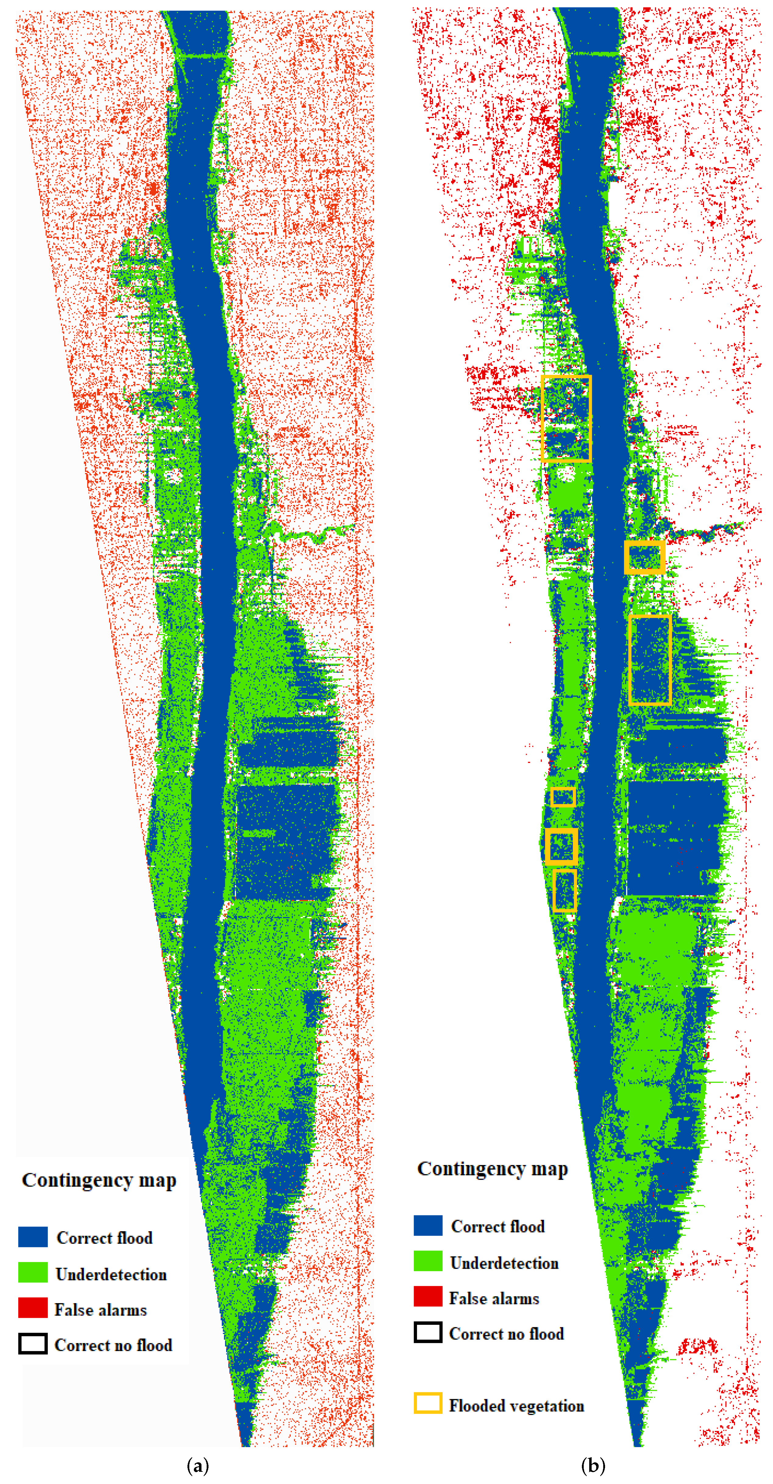
Evaluation Measures
5. Hydraulic Model Set-Up
6. Results
7. Discussion
8. Conclusions
Author Contributions
Funding
Acknowledgments
Conflicts of Interest
References
- Human Cost of Weather-Related Disasters 1995-2015; Technical Report; Centre for Research on the Epidemiology of Disasters (CRED); UN Office for Disaster Risk Reduction (UNISRD): Geneva, Switzerland, 2015.
- Estimate of the Average Annual Cost for Disaster Financial Assistance Arrangements due to Weather Events; Technical Report; Parliamentary Budget Officer: Ottawa, ON, Canada, 2016.
- Rapport D’évènement—Inondations Printanières Montérégie 2011; Technical Report; Organisation de la Sécurité Civile du Québec, Bibliothèque et Archives Nationales du Québec: Québec, QC, Canada, 2013.
- Rahman, M.S.; Di, L. The state of the art of spaceborne remote sensing in flood management. Nat. Hazards 2017, 85, 1223–1248. [Google Scholar] [CrossRef]
- Matgen, P.; Hostache, R.; Schumann, G.; Pfister, L.; Hoffmann, L.; Savenije, H. Towards an automated SAR-based flood monitoring system: Lessons learned from two case studies. Phys. Chem. Earth Part B 2011, 36, 241–252. [Google Scholar] [CrossRef]
- Landuyt, L.; Wesemael, A.; Schumann, G.J.P.; Hostache, R.; Verhoest, N.E.C.; Van Coillie, F.M.B. Synthetic Aperture Radar based flood mapping: an assessment of established approaches. IEEE Trans. Geosci. Remote Sens. 2018, in press. [Google Scholar] [CrossRef]
- Martinis, S.; Kersten, J.; Twele, A. A fully automated TerraSAR-X based flood service. ISPRS J. Photogramm. Remote Sens. 2015, 104, 203–212. [Google Scholar] [CrossRef]
- Pulvirenti, L.; Chini, M.; Pierdicca, N.; Guerriero, L.; Ferrazzoli, P. Flood monitoring using multi-temporal COSMO-SkyMed data: Image segmentation and signature interpretation. Remote Sens. Environ. 2011, 115, 990–1002. [Google Scholar] [CrossRef]
- Giustarini, L.; Hostache, R.; Matgen, P.; Schumann, G.J.P.; Bates, P.D.; Mason, D.C. A Change Detection Approach to Flood Mapping in Urban Areas Using TerraSAR-X. IEEE Trans. Geosci. Remote Sens. 2013, 51, 2417–2430. [Google Scholar] [CrossRef]
- Hostache, R.; Matgen, P.; Wagner, W. Change detection approaches for flood extent mapping: How to select the most adequate reference image from online archives? Int. J. Appl. Earth Obs. Geoinf. 2012, 19, 205–213. [Google Scholar] [CrossRef]
- Chini, M.; Hostache, R.; Giustarini, L.; Matgen, P. A Hierarchical Split-Based Approach (HSBA) for parametric thresholding of SAR images: flood inundation as a test case. IEEE Trans. Geosci. Remote Sens. 2017, 55, 6975–6988. [Google Scholar] [CrossRef]
- Lu, J.; Giustarini, L.; Xiong, B.; Zhao, L.; Jiang, Y.; Kuang, G. Automated flood detection with improved robustness and efficiency using multi-temporal SAR data. Remote Sens. Lett. 2014, 5, 240–248. [Google Scholar] [CrossRef]
- Giustarini, L.; Vernieuwe, H.; Verwaeren, J.; Chini, M.; Hostache, R.; Matgen, P.; Verhoest, N.; de Baets, B. Accounting for Image Uncertainty in SAR-based Flood Mapping. Int. J. Appl. Earth Obs. Geoinf. 2015, 34, 70–77. [Google Scholar] [CrossRef]
- Giustarini, L.; Hostache, R.; Kavetski, D.; Chini, M.; Corato, G.; Schlaffer, S.; Matgen, P. Probabilistic Flood Mapping Using Synthetic Aperture Radar Data. IEEE Trans. Geosci. Remote Sens. 2016, 54, 6958–6969. [Google Scholar] [CrossRef]
- Schlaffer, S.; Chini, M.; Giustarini, L.; Matgen, P. Probabilistic mapping of flood-induced backscatter changes in SAR time series. Int. J. Appl. Earth Obs. Geoinf. 2017, 56, 77–87. [Google Scholar] [CrossRef]
- Bazi, Y.; Bruzzone, L.; Melgani, F. An unsupervised approach based on the generalized Gaussian model to automatic change detection in multitemporal SAR images. IEEE Trans. Geosci. Remote Sens. 2005, 43, 874–887. [Google Scholar] [CrossRef]
- Kittler, J.; Illingworth, J. Minimum error thresholding. Pattern Recognit. 1986, 19, 41–47. [Google Scholar] [CrossRef]
- Pulvirenti, L.; Pierdicca, N.; Chini, M.; Guerriero, L. Monitoring flood evolution in vegetated areas using COSMO-SkyMed data: The Tuscany 2009 case study. IEEE J. Sel. Top. Appl. Earth Obs. Remote Sens. 2013, 6, 1807–1816. [Google Scholar] [CrossRef]
- Pierdicca, N.; Pulvirenti, L.; Chini, M. Flood Mapping in Vegetated and Urban Areas and Other Challenges: Models and Methods. In Flood Monitoring through Remote Sensing; Refice, A., D’Addabbo, A., Capolongo, D., Eds.; Springer: Cham, Switzerland, 2018; pp. 135–179. [Google Scholar]
- Pierdicca, N.; Pulvirenti, L.; Chini, M.; Guerriero, L.; Candela, L. Observing floods from space: Experience gained from COSMO-SkyMed observations. Acta Astronaut. 2013, 84, 122–133. [Google Scholar] [CrossRef]
- Mason, D.C.; Giustarini, L.; Garcia-Pintado, J.; Cloke, H.L. Detection of flooded urban areas in high resolution Synthetic Aperture Radar images using double scattering. Int. J. Appl. Earth Obs. Geoinf. 2014, 28, 150–159. [Google Scholar] [CrossRef]
- Chini, M.; Pulvirenti, L.; Pierdicca, N. Analysis and interpretation of the COSMO-SkyMed observations of the 2011 Japan tsunami. IEEE Geosci. Remote Sens. Lett. 2012, 9, 467–471. [Google Scholar] [CrossRef]
- Pulvirenti, L.; Chini, M.; Pierdicca, N.; Boni, G. Use of SAR data for detecting floodwater in urban and agricultural areas: The role of the interferometric coherence. IEEE Trans. Geosci. Remote Sens. 2016, 54, 1532–1544. [Google Scholar] [CrossRef]
- Selmi, S.; Abdallah, W.B.; Abdelfatteh, R. Flood mapping using InSAR coherence map. Int. Arch. Photogramm. Remote Sens. Spat. Inform. Sci. 2014, 40, 161. [Google Scholar] [CrossRef]
- Chaabani, C.; Abdelfattah, R. Optimized fuzzy algorithm based on modified similarity measure for mapping flood impacts. In Proceedings of the 2016 IEEE International Geoscience and Remote Sensing Symposium (IGARSS), Beijing, China, 10–15 July 2016; pp. 2380–2383. [Google Scholar]
- Chaabani, C.; Abdelfattah, R. InSAR Coherence-Dependent Fuzzy C-Means Flood Mapping Using Particle Swarm Optimization. In International Conference on Advanced Concepts for Intelligent Vision Systems; Springer: Cham, Switzerland, 2017; pp. 337–348. [Google Scholar]
- Martone, M.; Rizzoli, P.; Krieger, G. Volume decorrelation effects in TanDEM-X interferometric SAR data. IEEE Geosci. Remote Sens. Lett. 2016, 13, 1812–1816. [Google Scholar] [CrossRef]
- Rizzoli, P.; Martone, M.; Gonzalez, C.; Wecklich, C.; Tridon, D.B.; Bräutigam, B.; Bachmann, M.; Schulze, D.; Fritz, T.; Huber, M.; et al. Generation and performance assessment of the global TanDEM-X digital elevation model. ISPRS J. Photogramm. Remote Sens. 2017, 132, 119–139. [Google Scholar] [CrossRef]
- Martone, M.; Rizzoli, P.; Wecklich, C.; González, C.; Bueso-Bello, J.L.; Valdo, P.; Schulze, D.; Zink, M.; Krieger, G.; Moreira, A. The global forest/non-forest map from TanDEM-X interferometric SAR data. Remote Sens. Environ. 2018, 205, 352–373. [Google Scholar] [CrossRef]
- Plan Stratégique de DéVeloppement Durable Vision D’avenir 360 Portrait du Territoire. Technical Report. Administration Municipale de Saint-Jean-sur-Richelieu, Ville de Saint-Jean-sur-Richelieu 2015. Available online: http://ville.saint-jean-sur-richelieu.qc.ca/ planification-strategique/Documents/diagnostic-portrait-20151009.pdf (accessed on 9 October 2015).
- Riboust, P.; Brissette, F. Analysis of Lake Champlain/Richelieu River’s historical 2011 flood. Can. Water Resour. J. 2016, 41, 174–185. [Google Scholar] [CrossRef]
- Tanguy, M.; Chokmani, K.; Bernier, M.; Poulin, J.; Raymond, S. River flood mapping in urban areas combining Radarsat-2 data and flood return period data. Remote Sens. Environ. 2017, 198, 442–459. [Google Scholar] [CrossRef]
- Krieger, G.; Moreira, A.; Fiedler, H.; Hajnsek, I.; Werner, M.; Younis, M.; Zink, M. TanDEM-X: A satellite formation for high-resolution SAR interferometry. IEEE Trans. Geosci. Remote Sens. 2007, 45, 3317–3341. [Google Scholar] [CrossRef]
- Hostache, R.; Matgen, P.; Giustarini, L.; Teferle, F.N.; Tailliez, C.; Iffly, J.F.; Corato, G. A drifting GPS buoy for retrieving effective riverbed bathymetry. J. Hydrol. 2015, 520, 397–406. [Google Scholar] [CrossRef]
- Martone, M.; Bräutigam, B.; Rizzoli, P.; Gonzalez, C.; Bachmann, M.; Krieger, G. Coherence evaluation of TanDEM-X interferometric data. ISPRS J. Photogramm. Remote Sens. 2012, 73, 21–29. [Google Scholar] [CrossRef]
- Breiman, L. Random forests. Mach. Learn. 2001, 45, 5–32. [Google Scholar] [CrossRef]
- Myint, S.W.; Okin, G.S. Modelling land-cover types using Multiple Endmember Spectral Mixture Analysis in a desert city. Int. J. Remote Sens. 2009, 30, 2237–2257. [Google Scholar] [CrossRef]
- Liu, T.; Yang, X. Mapping vegetation in an urban area with stratified classification and multiple endmember spectral mixture analysis. Remote Sens. Environ. 2013, 133, 251–264. [Google Scholar] [CrossRef]
- Sonobe, R.; Tani, H.; Wang, X.; Kobayashi, N.; Shimamura, H. Random forest classification of crop type using multi-temporal TerraSAR-X dual-polarimetric data. Remote Sens. Lett. 2014, 5, 157–164. [Google Scholar] [CrossRef]
- Dubeau, P.; King, D.J.; Unbushe, D.G.; Rebelo, L.M. Mapping the Dabus Wetlands, Ethiopia, Using Random Forest Classification of Landsat, PALSAR and Topographic Data. Remote Sens. 2017, 9, 1056. [Google Scholar] [CrossRef]
- Feng, Q.; Gong, J.; Liu, J.; Li, Y. Flood mapping based on multiple endmember spectral mixture analysis and random forest classifier—The case of Yuyao, China. Remote Sens. 2015, 7, 12539–12562. [Google Scholar] [CrossRef]
- Wohlfart, C.; Winkler, K.; Wendleder, A.; Roth, A. TerraSAR-X and Wetlands: A Review. Remote Sens. 2018, 10, 916. [Google Scholar] [CrossRef]
- Waske, B.; van der Linden, S. Classifying multilevel imagery from SAR and optical sensors by decision fusion. IEEE Trans. Geosci. Remote Sens. 2008, 46, 1457–1466. [Google Scholar] [CrossRef]
- Pierdicca, N.; Chini, M.; Pelliccia, F. The contribution of SIASGE radar data integrated with optical images to support thematic mapping at regional scale. IEEE J. Sel. Top. Appl. Earth Obs. Remote Sens. 2014, 7, 2821–2833. [Google Scholar] [CrossRef]
- Aggarwal, C.C. Data Mining: The Textbook. Springer Publishing Company, Incorporated, 2015. Available online: https://www.springer.com/de/book/9783319141411 (accessed on 1 January 2015).
- Breiman, L. Bagging predictors. Mach. Learn. 1996, 24, 123–140. [Google Scholar] [CrossRef]
- Safavian, S.R.; Landgrebe, D. A survey of decision tree classifier methodology. IEEE Trans. Syst. Man Cybern. 1991, 21, 660–674. [Google Scholar] [CrossRef]
- Bates, P.D.; De Roo, A. A simple raster-based model for flood inundation simulation. J. Hydrol. 2000, 236, 54–77. [Google Scholar] [CrossRef]
- Horritt, M.; Bates, P. Evaluation of 1D and 2D numerical models for predicting river flood inundation. J. Hydrol. 2002, 268, 87–99. [Google Scholar] [CrossRef]
- Afshari, S.; Tavakoly, A.A.; Rajib, M.A.; Zheng, X.; Follum, M.L.; Omranian, E.; Fekete, B.M. Comparison of new generation low-complexity flood inundation mapping tools with a hydrodynamic model. J. Hydrol. 2018, 556, 539–556. [Google Scholar] [CrossRef]
- Neal, J.; Schumann, G.; Fewtrell, T.; Budimir, M.; Bates, P.; Mason, D. Evaluating a new LISFLOOD-FP formulation with data from the summer 2007 floods in Tewkesbury, UK. J. Flood Risk Manag. 2011, 4, 88–95. [Google Scholar] [CrossRef]
- Van der Sande, C.; De Jong, S.; De Roo, A. A segmentation and classification approach of IKONOS-2 imagery for land cover mapping to assist flood risk and flood damage assessment. Int. J. Appl. Earth Obs. Geoinf. 2003, 4, 217–229. [Google Scholar] [CrossRef]
- Wood, M.; Hostache, R.; Neal, J.; Wagener, T.; Giustarini, L.; Chini, M.; Corato, G.; Matgen, P.; Bates, P. Calibration of channel depth and friction parameters in the LISFLOOD-FP hydraulic model using medium-resolution SAR data and identifiability techniques. Hydrol. Earth Syst. Sci. 2016, 20, 4983. [Google Scholar] [CrossRef]
- Hostache, R.; Chini, M.; Giustarini, L.; Neal, J.; Kavetski, D.; Wood, M.; Corato, G.; Pelich, R.M.; Matgen, P. Near-Real-Time Assimilation of SAR-Derived Flood Maps for Improving Flood Forecasts. Water Resour. Res. 2018, 54, 5516–5535. [Google Scholar] [CrossRef]
- Hostache, R.; Hissler, C.; Matgen, P.; Guignard, C.; Bates, P. Modelling suspended-sediment propagation and related heavy metal contamination in floodplains: A parameter sensitivity analysis. Water Resour. Res. 2014, 18, 3539–3551. [Google Scholar]
- Oubennaceur, K.; Chokmani, K.; Nastev, M.; Tanguy, M.; Raymond, S. Uncertainty Analysis of a Two-Dimensional Hydraulic Model. Water 2018, 10, 272. [Google Scholar] [CrossRef]
- Congalton, R.G. A review of assessing the accuracy of classifications of remotely sensed data. Remote Sens. Environ. 1991, 37, 35–46. [Google Scholar] [CrossRef]
- Brisco, B.; Schmitt, A.; Murnaghan, K.; Kaya, S.; Roth, A. SAR polarimetric change detection for flooded vegetation. Int. J. Digit. Earth 2013, 6, 103–114. [Google Scholar] [CrossRef]
- Chini, M.; Papastergios, A.; Pulvirenti, L.; Pierdicca, N.; Matgen, P.; Parcharidis, I. SAR coherence and polarimetric information for improving flood mapping. In Proceedings of the 2016 IEEE International Geoscience and Remote Sensing Symposium (IGARSS), Beijing, China, 10–15 July 2016; pp. 7577–7580. [Google Scholar]


| Acquisition Time | Acquisition Mode | Polarization | Looking Angle | |
|---|---|---|---|---|
| 14/05/2011 (during the flood) | Stripmap (Ascending) | HH | 318.02 | 41–43 |
| 14/07/2011 (after the flood) | Stripmap (Ascending) | HH | 281.36 | 39–41 |
| 29/08/2012 (after the flood) | Stripmap (Ascending) | HH | 407.49 | 40–42 |
| Date | May 2011 (Flooding Period) | July 2011 | August 2012 | |||
|---|---|---|---|---|---|---|
| Intensity | InSAR Coh. | Intensity | InSAR Coh. | Intensity | InSAR Coh. | |
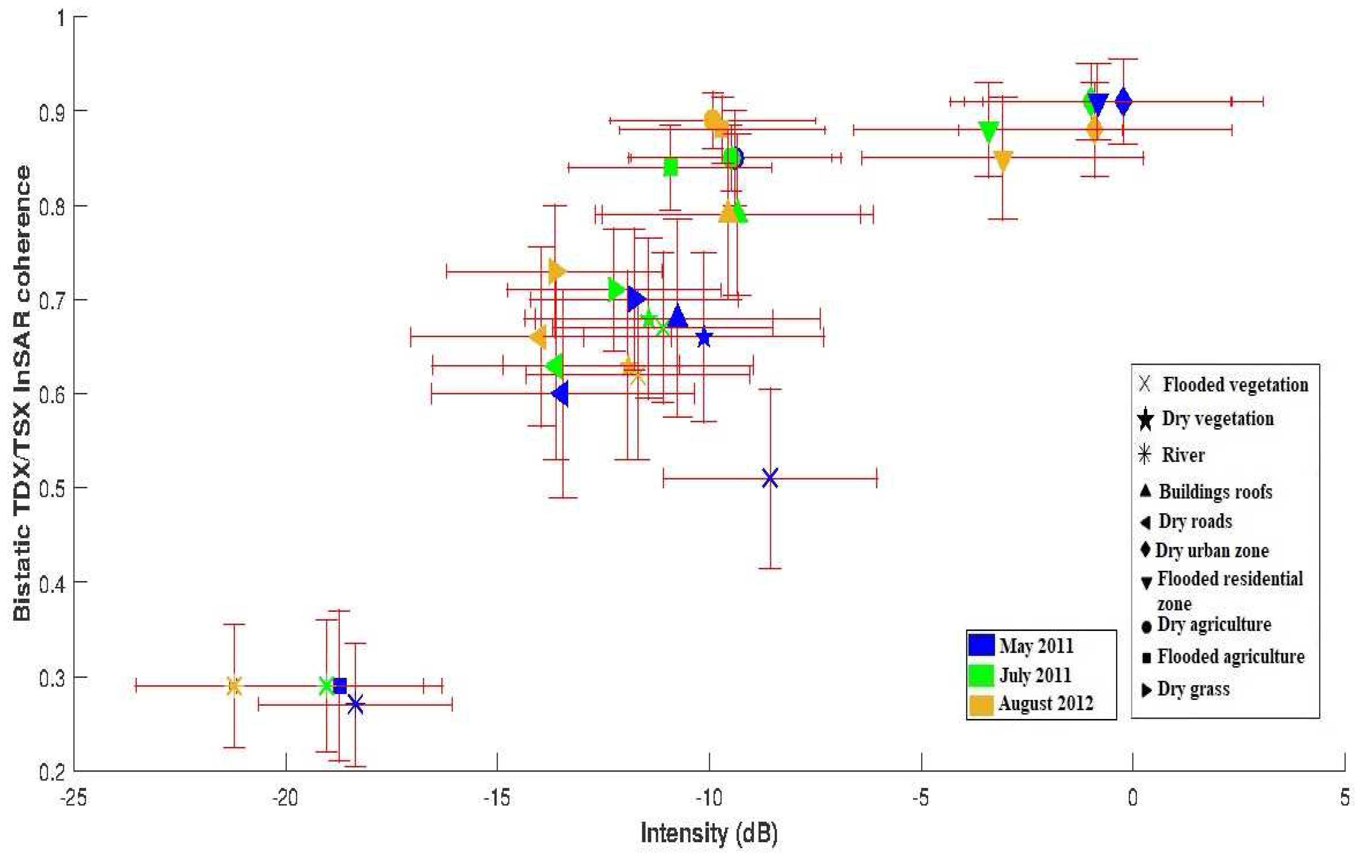
| 1: River | −18.36 (4.56) | 0.27 (0.13) | −19.04 (4.59) | 0.29 0.14 | −21.21 (4.65) | 0.29 (0.13) |
| 2: Dry agriculture | −9.54 (5.02) | 0.85 (0.1) | −9.46 (4.72) | 0.85 (0.07) | −9.92 (4.86) | 0.89 (0.06) |
| 3: Flooded agriculture | −18.73 (4.85) | 0.29 (0.16) | −10.93 (4.79) | 0.84 (0.09) | −9.69 (4.84) | 0.88 (0.07) |
| 4: Dry vegetation | −10.13 (5.67) | 0.66 (0.18) | −11.43 (5.87) | 0.68 (0.17) | −11.92 (5.9) | 0.63 (0.2) |
| 5: Flooded vegetation | −8.56 (5.04) | 0.51 (0.19) | −11.10 (5.19) | 0.67 (0.16) | −11.68 (5.27) | 0.62 (0.18) |
| 6: Dry urban | −0.24 (6.6) | 0.91 (0.09) | −1.05 (6.64) | 0.91 (0.08) | −0.9 (6.46) | 0.88 (0.1) |
| 7: Dry roads | −13.46 (6.2) | 0.6 (0.22) | −13.62 (5.85) | 0.63 (0.2) | −13.97 (6.15) | 0.66 (0.19) |
| 8: Dry grass | −11.77 (4.92) | 0.7 (0.15) | −12.25 (5.04) | 0.71 (0.13) | −13.65 (5.09) | 0.73 (0.14) |
| 9: Buildings roofs | −18.36 (6.71) | 0.27 (0.21) | −19.04 (6.4) | 0.29 (0.17) | −21.21 (6.26) | 0.29 (0.18) |
| 10: Flooded residential | −0.87 (6.31) | 0.91 (0.08) | −3.47 (6.35) | 0.88 (0.1) | −3.13 (6.65) | 0.85 (0.13) |
| Ground Truth | |||
|---|---|---|---|
| Flood | No Flood | ||
| Model | Flood | a: True positive | b: False positive |
| No Flood | c: False negative | d: True negative | |
| Critical Success Index (CSI) | Overall Accuracy (OA) | |
|---|---|---|
| performance value |
| Multi-Temporal Input Data | Training Parameters | Overall Accuracy | Precision | |
|---|---|---|---|---|
| Samples Number | Decision Trees | |||
| Intensity only | 15,000 | 100 | 69.69% | 64.97% |
| Intensity and Bist. TDX/TSX InSAR Coh. | 15,000 | 100 | 78.69% | 80.34% |
| Intensity only | 20,000 | 100 | 69.58% | 64.65% |
| Intensity and Bist. TDX/TSX InSAR Coh. | 20,000 | 100 | 78.59% | 81.06% |
| Intensity only | 20,000 | 300 | 69.63% | 64.52% |
| Intensity and Bist. TDX/TSX InSAR Coh. | 20,000 | 300 | 78.65% | 82.08% |
| Intensity only | 20,000 | 500 | 70.07% | 65.64% |
| Intensity and Bist. TDX/TSX InSAR Coh. | 20,000 | 500 | 78.66% | 81.95% |
© 2018 by the authors. Licensee MDPI, Basel, Switzerland. This article is an open access article distributed under the terms and conditions of the Creative Commons Attribution (CC BY) license (http://creativecommons.org/licenses/by/4.0/).
Share and Cite
Chaabani, C.; Chini, M.; Abdelfattah, R.; Hostache, R.; Chokmani, K. Flood Mapping in a Complex Environment Using Bistatic TanDEM-X/TerraSAR-X InSAR Coherence. Remote Sens. 2018, 10, 1873. https://doi.org/10.3390/rs10121873
Chaabani C, Chini M, Abdelfattah R, Hostache R, Chokmani K. Flood Mapping in a Complex Environment Using Bistatic TanDEM-X/TerraSAR-X InSAR Coherence. Remote Sensing. 2018; 10(12):1873. https://doi.org/10.3390/rs10121873
Chicago/Turabian StyleChaabani, Chayma, Marco Chini, Riadh Abdelfattah, Renaud Hostache, and Karem Chokmani. 2018. "Flood Mapping in a Complex Environment Using Bistatic TanDEM-X/TerraSAR-X InSAR Coherence" Remote Sensing 10, no. 12: 1873. https://doi.org/10.3390/rs10121873
APA StyleChaabani, C., Chini, M., Abdelfattah, R., Hostache, R., & Chokmani, K. (2018). Flood Mapping in a Complex Environment Using Bistatic TanDEM-X/TerraSAR-X InSAR Coherence. Remote Sensing, 10(12), 1873. https://doi.org/10.3390/rs10121873