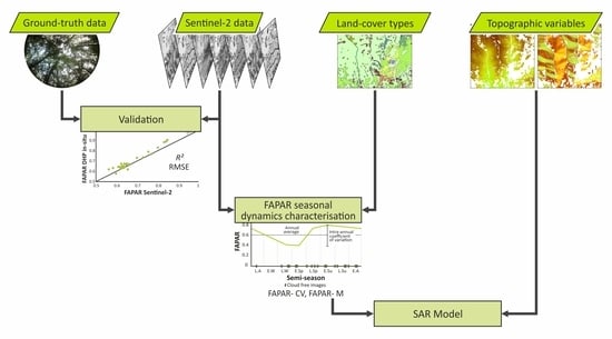
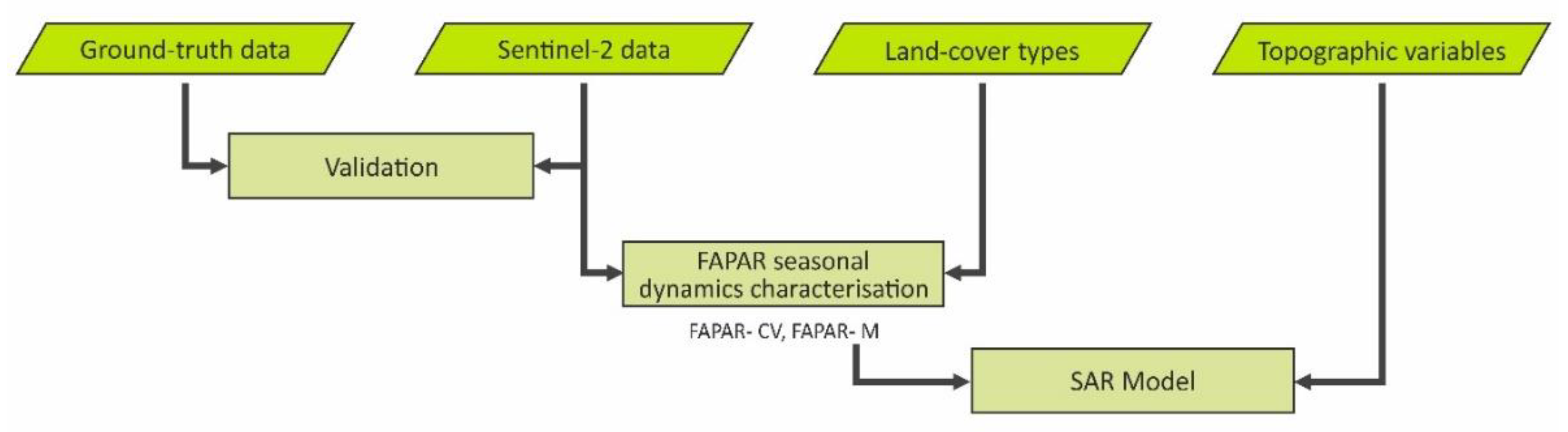
Figure 1.
Flow chart of the methodology.
Figure 1.
Flow chart of the methodology.
Figure 2.
Types and canopy coverages (cc) of the land covers in the study site. The percentage of the area of each land cover type over the entire study site is shown in detail. Data obtained from the Land Cover Map of Catalonia [
21]. Reference System ETRS89 Universal Transverse Mercator (UTM) zone 31 N.
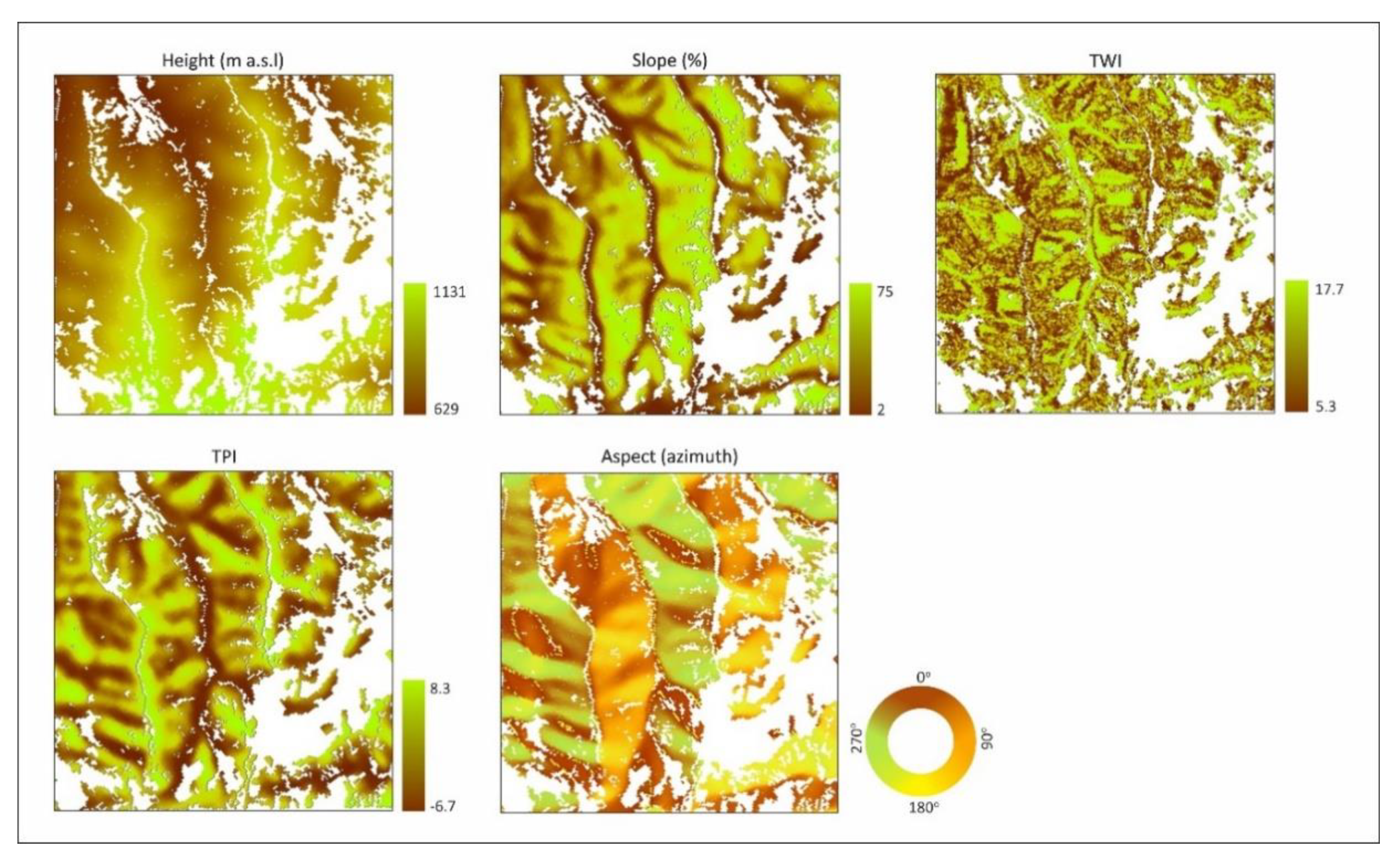
Figure 3.
Topographic variables obtained and derived from the digital elevation model (DEM) for the main vegetation cover type at the study site (evergreen oak forest, Quercus ilex): height (metres above sea level), slope (in percentage), Topographic Wetness Index (TWI), Topographic Position Index (TPI) and topographic aspect (azimuth that slopes are facing: 0° north, 90° east, 180° south, 270° west).
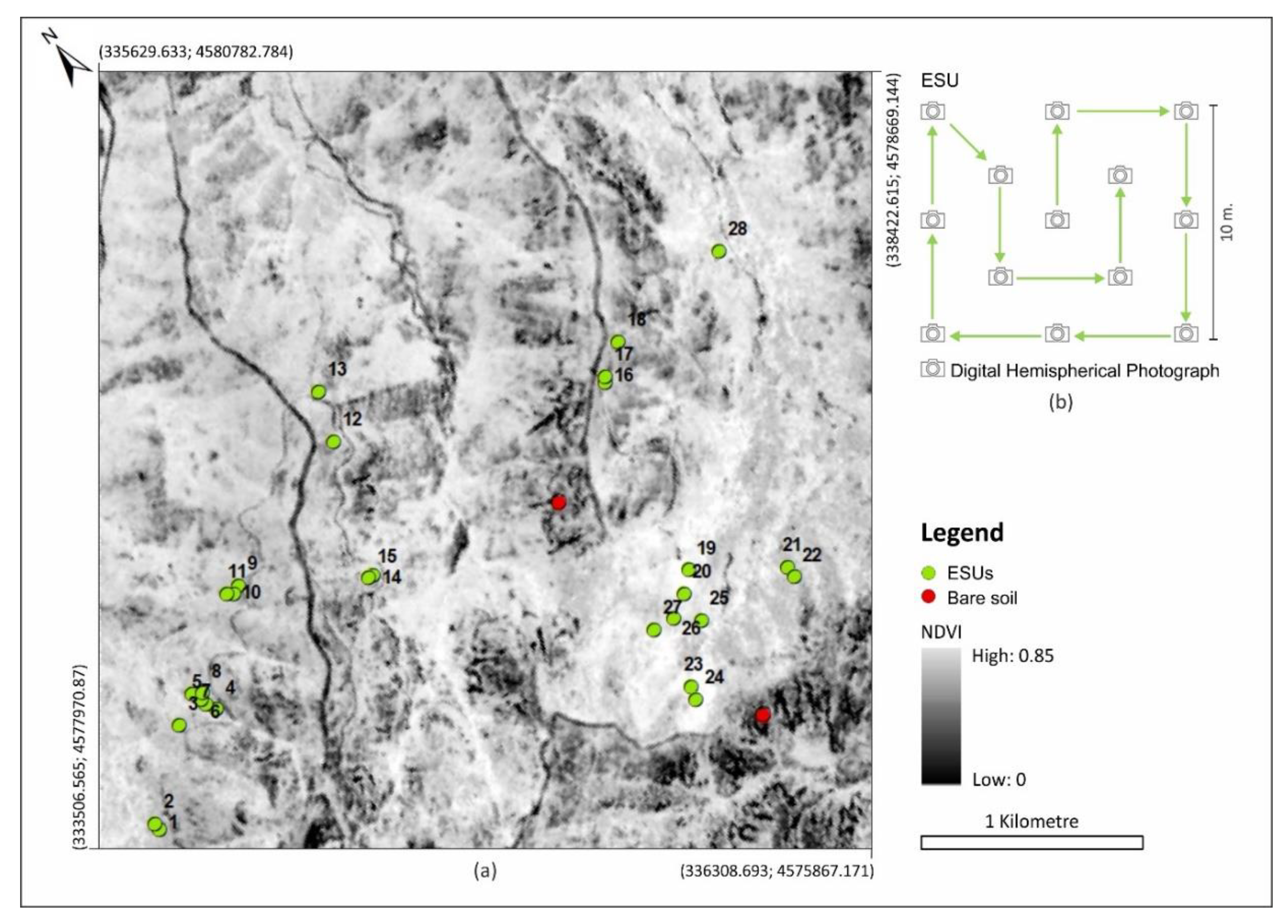
Figure 4.
(a) Normalized Difference Vegetation Index (NDVI) cartography for the study area (satellite imagery acquired on 12 June 2017) indicating the location of the 28 elementary sampling units (ESUs) and the two additional units of bare soil. Reference System ETRS89 UTM zone 31 N. (b) The sampling scheme of the measurements within an ESU is shown in detail, where arrows indicate the path followed during the sampling.
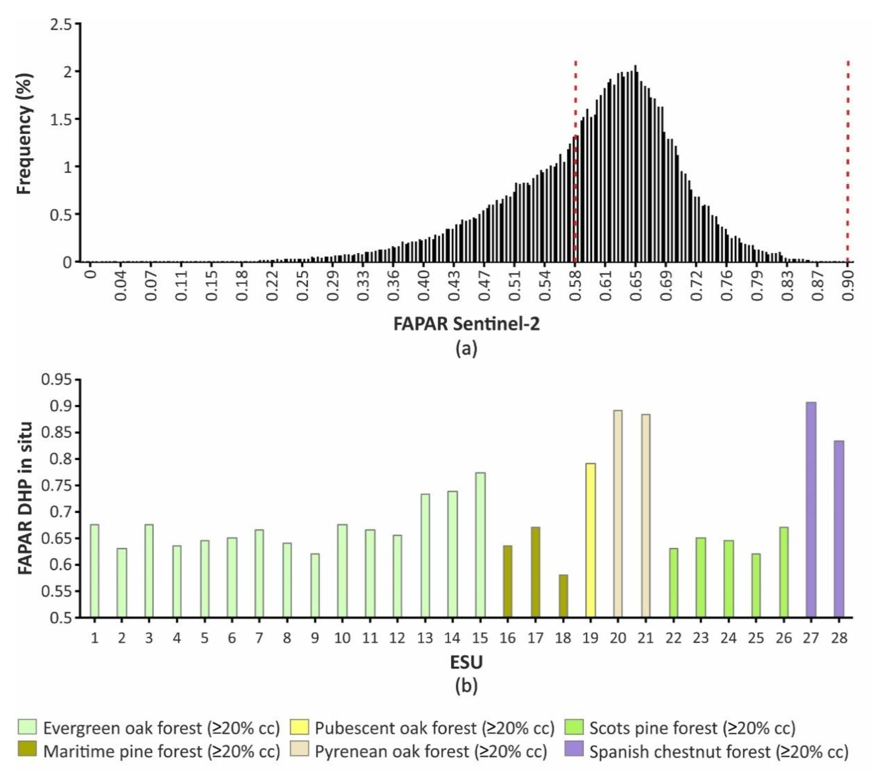
Figure 5.
(a) Frequency distribution of the fraction of absorbed photosynthetically active radiation (FAPAR) from Sentinel-2 satellite images for the study site and sampling period (three days between satellite acquisition and the ground measurements). The red dotted line indicates the FAPAR range sampled in situ. (b) FAPAR ground measurements obtained from digital hemispherical photography (DHP) for each elementary sampling unit (ESU) by type and canopy coverage (cc) of land cover.
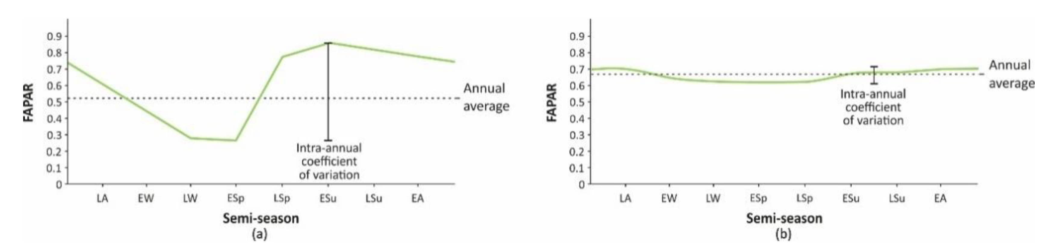
Figure 6.
Examples of the seasonal dynamics of the fraction of absorbed photosynthetically active radiation (FAPAR) for two systems with: (a) moderate annual magnitude and high seasonal variability; and (b) high annual magnitude and low seasonal variability. LA, late autumn; EW, early winter; LW, late winter; ESp, early spring; LSp, late spring; ESu, early summer; LSu, late summer; EA, early autumn.
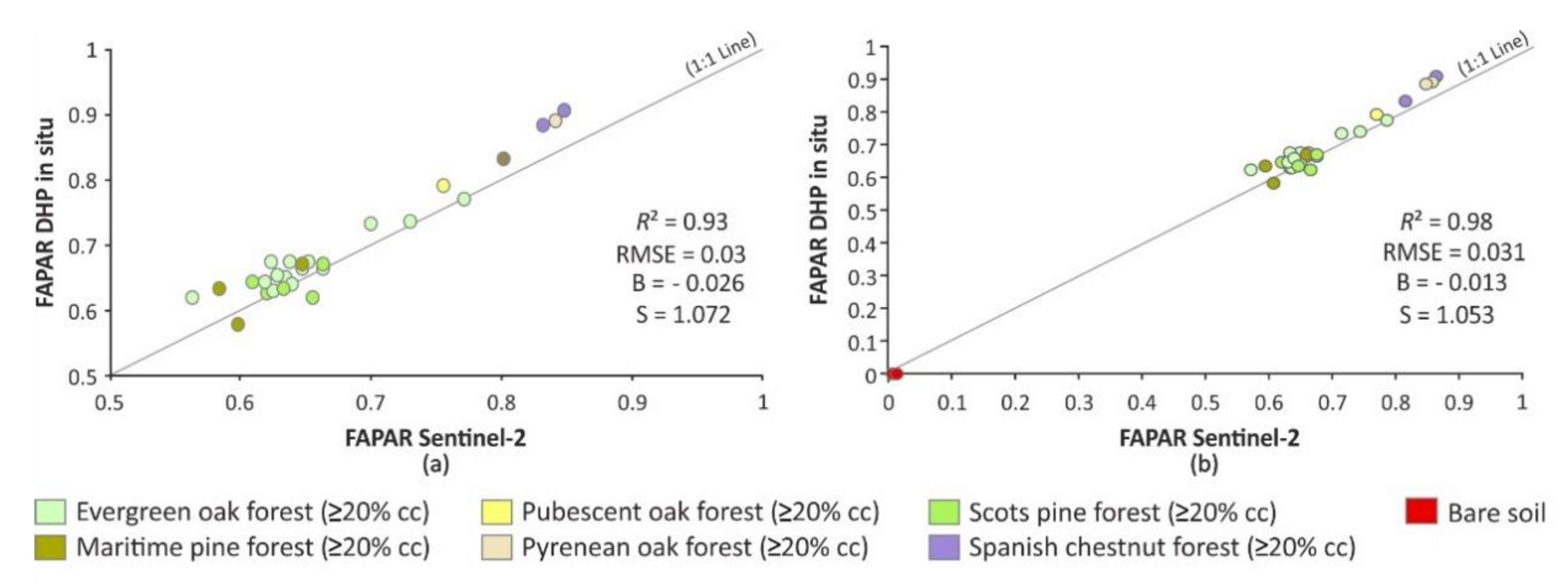
Figure 7.
Scatter-plots between ground measurements obtained from digital hemispherical photography (DHP) and the corresponding fraction of absorbed photosynthetically active radiation (FAPAR) from Sentinel-2 satellite images. FAPAR ground measurements for each elementary sampling unit by type and canopy coverage (cc) of land cover is shown in detail. (a) Only ground-truth elementary sampling unit data (n = 28), (b) with the extra units of bare soil obtained from very-high-resolution satellite imagery (n = 30).
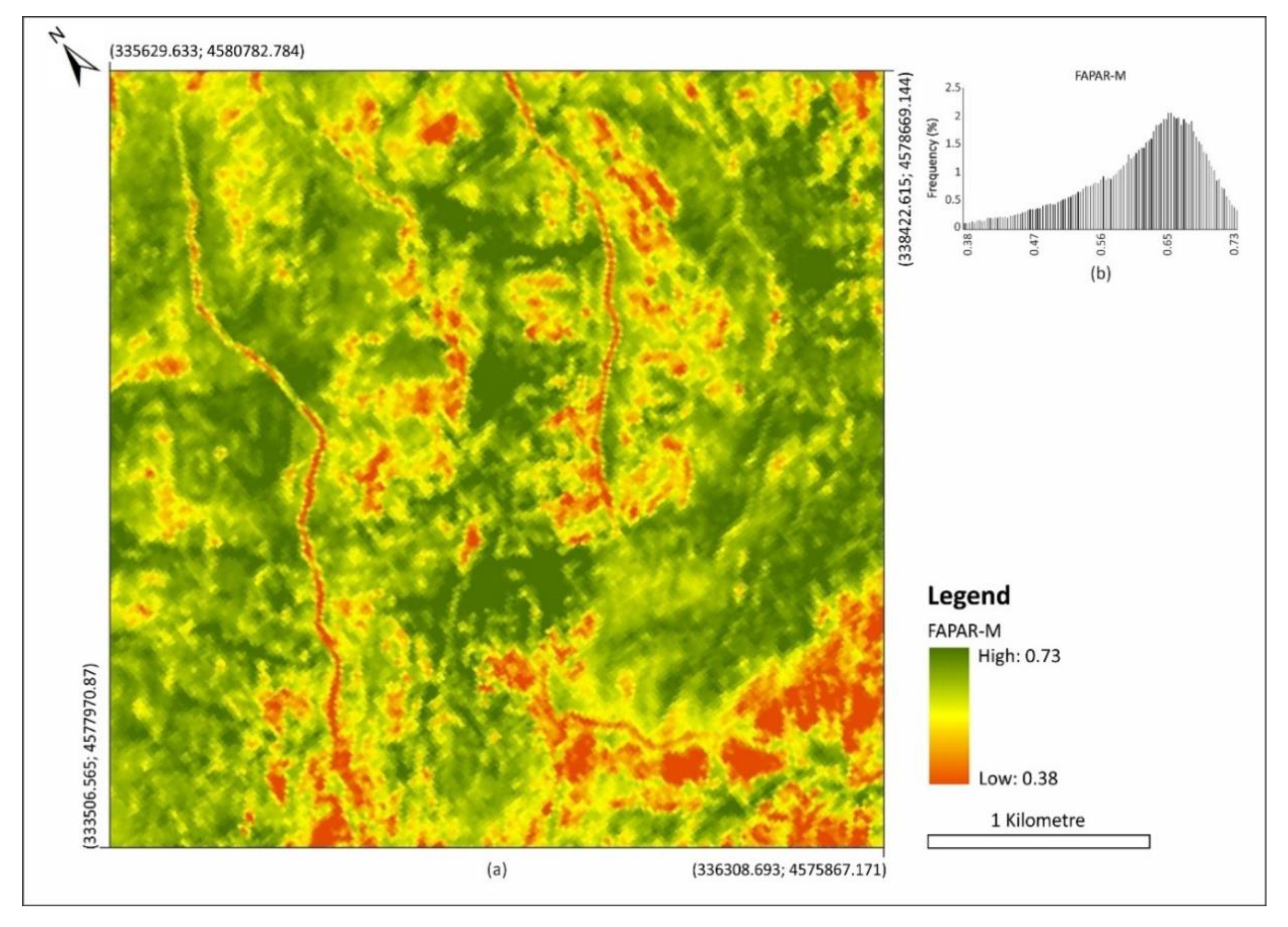
Figure 8.
(a) Geographically explicit data set for the annual magnitude of the fraction of absorbed photosynthetically active radiation (FAPAR-M), derived from the seasonal curves of FAPAR obtained with one year of data (2016/2017) from the Multispectral Instrument (MSI) on the Sentinel-2 satellite. Reference System ETRS89 UTM zone 31 N. (b) Negatively skewed frequency distribution of FAPAR-M between the 2.5 (0.38) and 97.5 (0.73) percentiles.
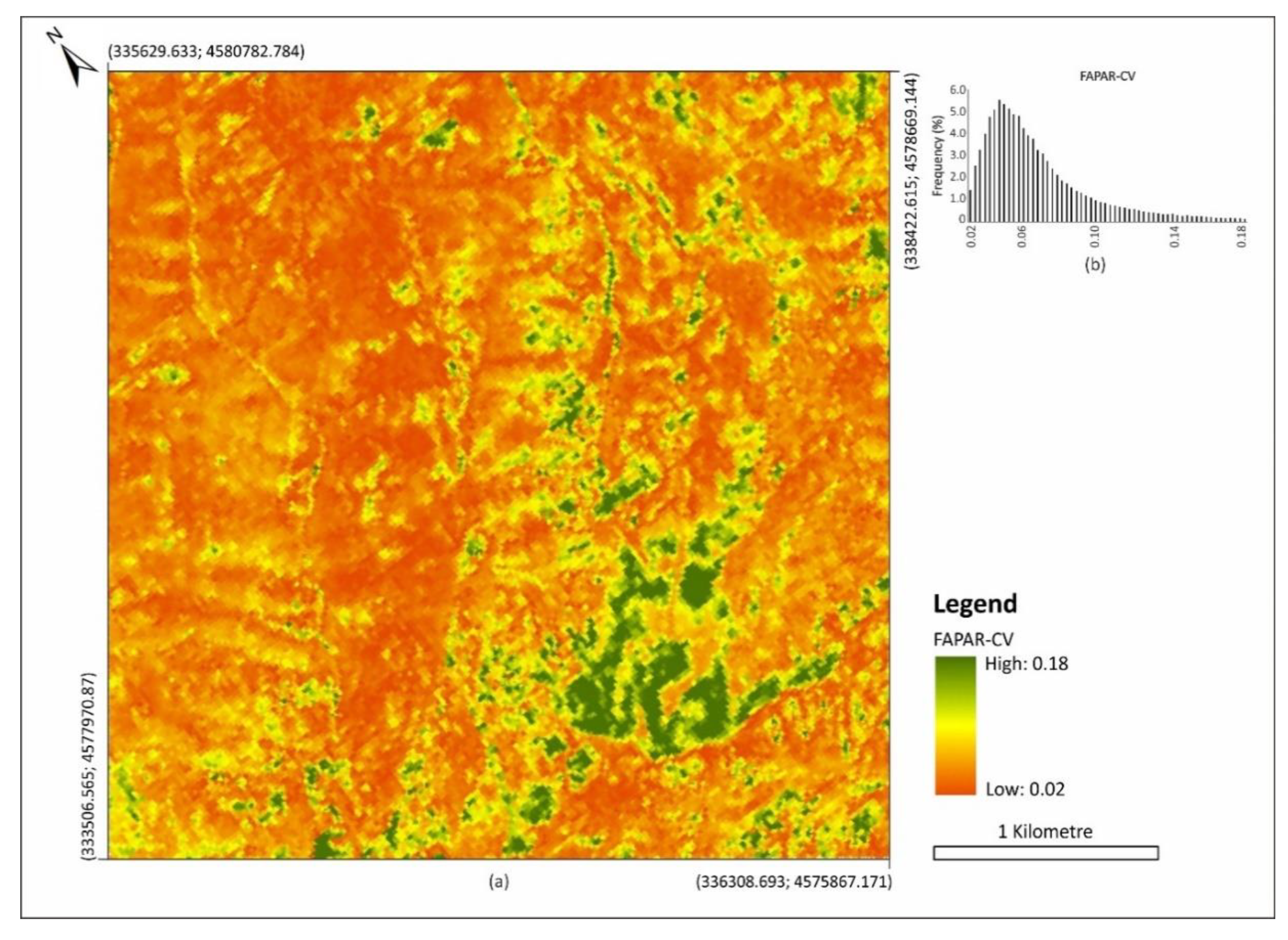
Figure 9.
(a) Geographically explicit data set for the seasonality of the fraction of absorbed photosynthetically active radiation (FAPAR-CV), derived from the seasonal curves of FAPAR obtained with one year of data (2016/2017) from the Multispectral Instrument on the Sentinel-2 satellite. Reference System ETRS89 UTM zone 31 N. (b) Positively skewed frequency distribution of FAPAR-CV between the 2.5 (0.02) and 97.5 (0.18) percentiles.
Figure 10.
Seasonal curves of the fraction of absorbed photosynthetically active radiation (FAPAR) for the main types and canopy coverages (cc) of land cover, obtained from one year of data (2016/2017) from the Multispectral Instrument on the Sentinel-2 satellite and the Land Cover Map of Catalonia. The error bars indicate the spatial standard deviation. LA, late autumn; EW, early winter; LW, late winter; ESp, early spring; LSp, late spring; ESu, early summer; LSu, late summer; EA, early autumn.
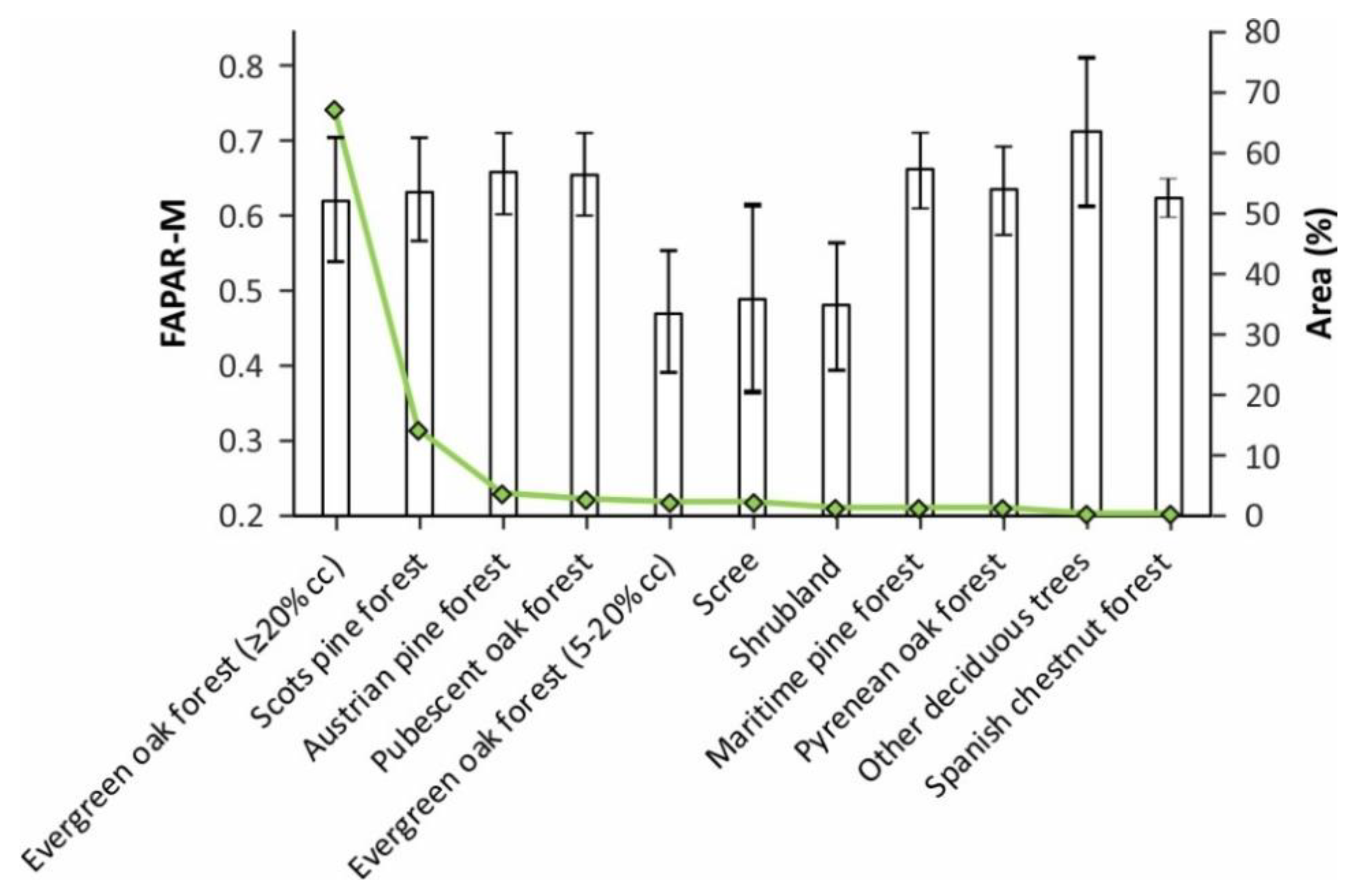
Figure 11.
Annual magnitude of the fraction of absorbed photosynthetically active radiation (FAPAR-M) for the main types and canopy coverages (cc) of land cover. The bars correspond to mean FAPAR-M, and the error bars correspond to the spatial standard deviation. The green line corresponds to the percentage of the area of each cover type over the entire study site (see
Section 2.1).
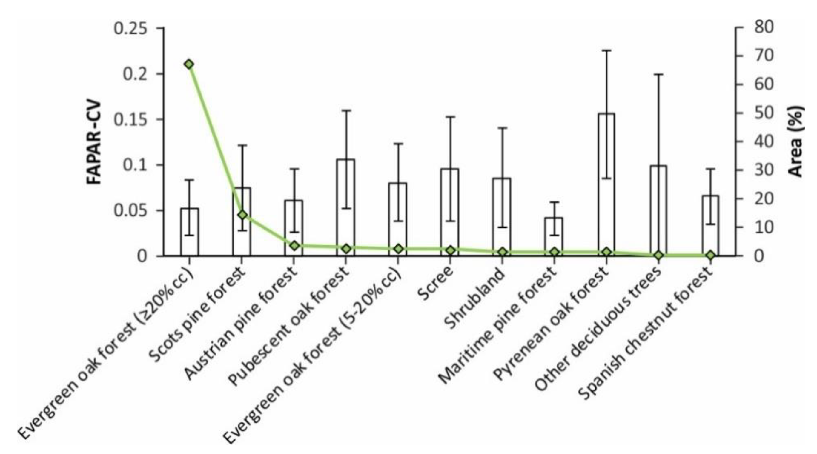
Figure 12.
Seasonality of the fraction of absorbed photosynthetically active radiation (FAPAR-CV) for the main types and canopy coverages (cc) of land cover. The bars correspond to mean FAPAR-CV, and the error bars correspond to the spatial standard deviation. The green line corresponds to the percentage of the area of each cover type over the entire study site (see
Section 2.1).
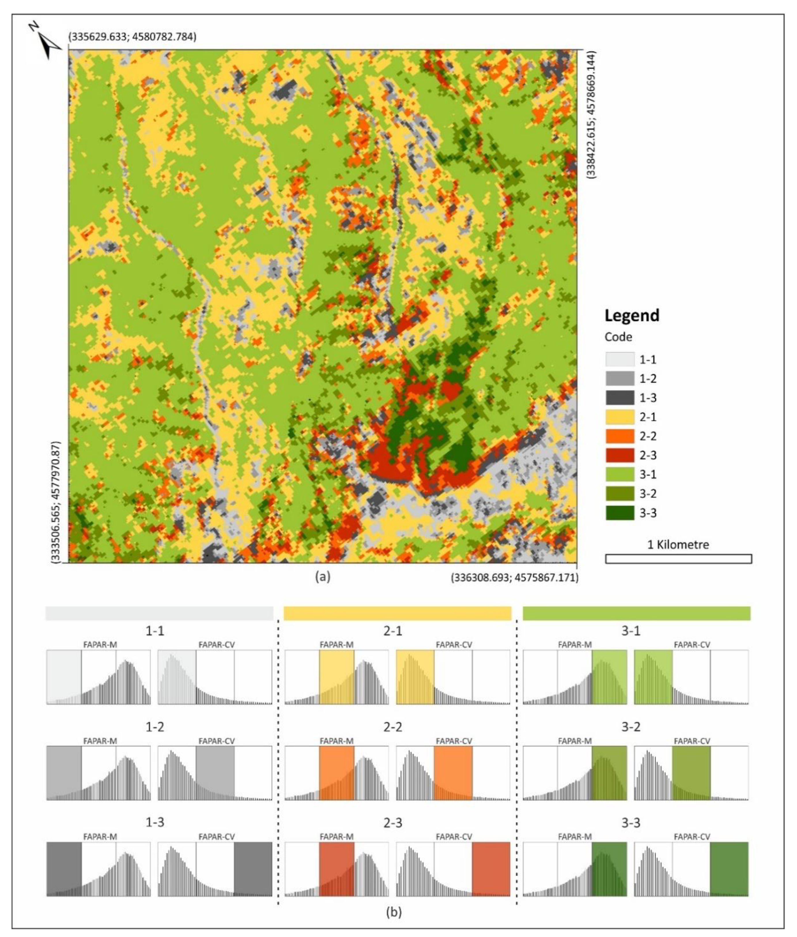
Figure 13.
(a) Map of the vegetation groups with different dynamics of absorption of photosynthetically active radiation for 2016-2017 obtained from the seasonal curves of the Sentinel-2 satellite data. Reference System ETRS89 UTM zone 31 N. (b) Each group is defined by a two-number code. The first and second numbers (1 = low, 2 = medium, 3 = high) indicate the magnitude and seasonality of the fraction of absorbed photosynthetically active radiation, respectively.
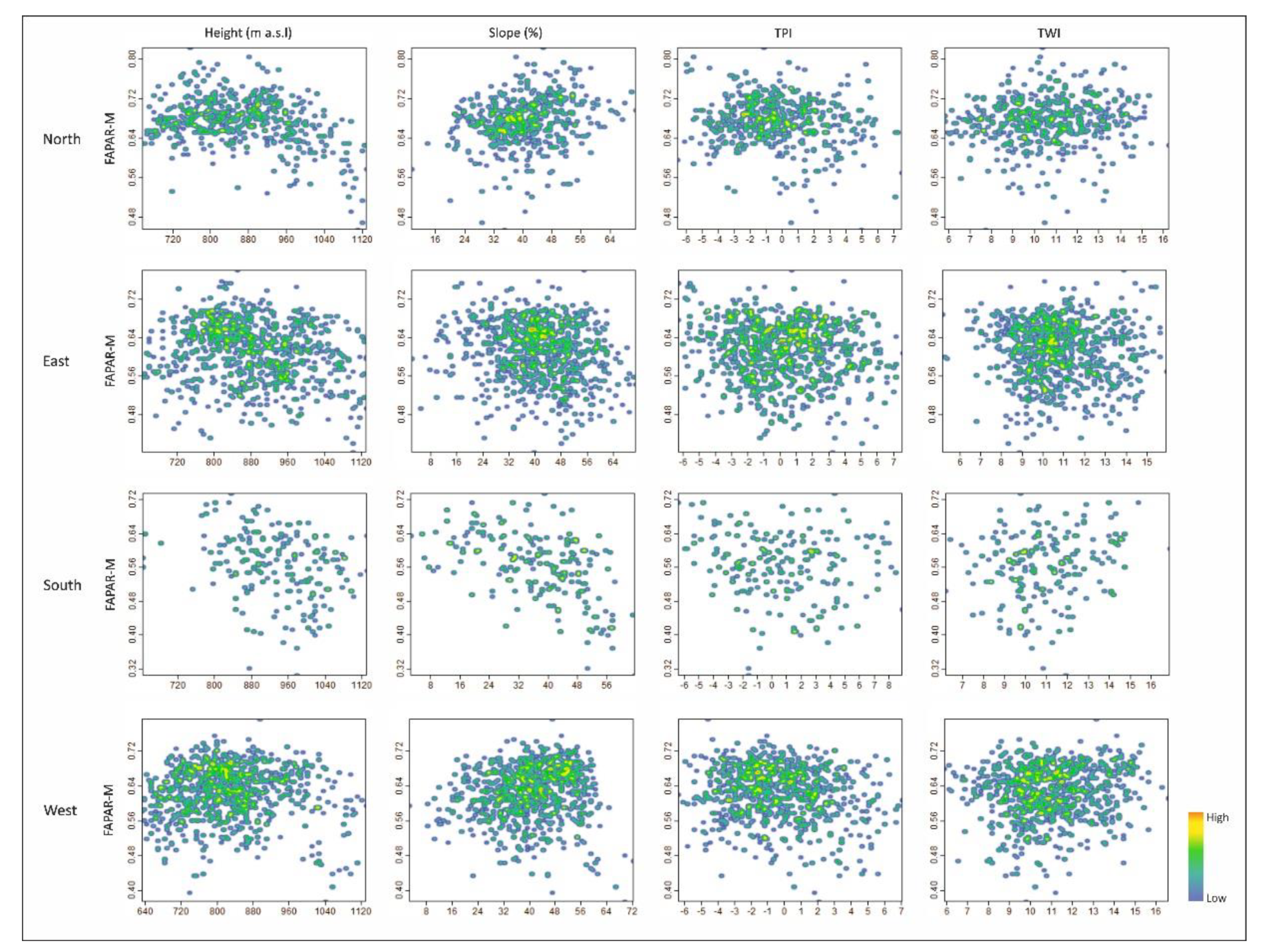
Figure 14.
Density scatter-plots between FAPAR-M of the main type of land cover, evergreen oak forest (Quercus ilex), and the topographic variables: height (metres above sea level), slope (in percentage), Topographic Wetness Index (TWI) and Topographic Position Index (TPI), analysed for the topographic aspects.
Table 1.
Cloud-free satellite images for each semi-season composite.
Table 1.
Cloud-free satellite images for each semi-season composite.
| Semi-Season Product | Start | End | Cloud-Free Satellite Images |
|---|
| Late autumn | 6 November | 20 December | 17 November | | | | |
| Early winter | 21 December | 3 February | | | | | |
| Late winter | 4 February | 20 March | 25 February | 14 March | 17 March | | |
| Early spring | 21 March | 5 May | 3 April | 6 April | | | |
| Late spring | 6 May | 20 June | 6 May | 16 May | 26 May | 12 June | |
| Early summer | 21 June | 4 August | 2 July | 5 July | 4 August | | |
| Late summer | 5 August | 20 September | 11 August | 14 August | 10 September | 13 September | 20 September |
| Early autumn | 21 September | 5 November | 10 October | 13 October | | | |
Table 2.
Areas of the vegetation groups with different dynamics of absorption of photosynthetically active radiation for 2016-2017.
Table 2.
Areas of the vegetation groups with different dynamics of absorption of photosynthetically active radiation for 2016-2017.
| Group Code | Area (ha) | Area (%) |
|---|
| 1-1 | 60.00 | 4.90 |
| 1-2 | 52.32 | 4.27 |
| 1-3 | 32.67 | 2.67 |
| 2-1 | 278.24 | 22.71 |
| 2-2 | 80.34 | 6.56 |
| 2-3 | 36.24 | 2.96 |
| 3-1 | 567.96 | 46.36 |
| 3-2 | 92.55 | 7.56 |
| 3-3 | 24.67 | 2.01 |
Table 3.
Correspondence between the vegetation groups with different dynamics of absorption of photosynthetically active radiation and the land-cover types across the study site.
Table 3.
Correspondence between the vegetation groups with different dynamics of absorption of photosynthetically active radiation and the land-cover types across the study site.
| Group Code | Land-Cover Type (Canopy Coverage) | Area (ha) (% area) | Correspondence (%) |
|---|
| 1-1 | Evergreen oak forest (≥20%) | 36.1 (4.4) | 60 |
| | Evergreen oak forest (5–20%) | 6.6 (22.5) | 11 |
| | Scree | 5.1 (19.1) | 8 |
| | Shrubland | 4.5 (24.6) | 7 |
| | Other | | 14 |
| 1-2 | Evergreen oak forest (≥20%) | 26 (3.2) | 50 |
| | Evergreen oak forest (5–20%) | 7.9 (26.9) | 15 |
| | Scree | 5.4 (20.2) | 10 |
| | Shrubland | 5 (27.4) | 10 |
| | Other | | 15 |
| 1-3 | Evergreen oak forest (≥20%) | 10.7 (1.3) | 33 |
| | Scots pine forest (≥20%) | 5.9 (3.4) | 18 |
| | Shrubland | 4.4 (24.1) | 13 |
| | Scree | 4 (15.0) | 12 |
| | Evergreen oak forest (5–20%) | 3.6 (12.3) | 11 |
| | Other | | 13 |
| 2-1 | Evergreen oak forest (≥20%) | 222.7 (27.4) | 80 |
| | Scots pine forest (≥20%) | 20.6 (11.7) | 7 |
| | Other | | 13 |
| 2-2 | Evergreen oak forest (≥20%) | 49.8 (6.1) | 62 |
| | Scots pine forest (≥20%) | 15 (8.5) | 19 |
| | Other | | 19 |
| 2-3 | Scots pine forest (≥20%) | 12.2 (6.9) | 34 |
| | Evergreen oak forest (≥20%) | 8.5 (1.0) | 23 |
| | Pyrenean oak forest (≥20%) | 5.2 (32.1) | 14 |
| | Pubescent oak forest (≥20%) | 3.4 (10.1) | 9 |
| | Scree | 2.3 (8.6) | 6 |
| | Other | | 14 |
| 3-1 | Evergreen oak forest (≥20%) | 408.9 (50.3) | 72 |
| | Scots pine forest (≥20%) | 89.4 (50.9) | 16 |
| | Austrian pine forest (≥20%) | 29.5 (65.2) | 5 |
| | Other | | 7 |
| 3-2 | Evergreen oak forest (≥20%) | 46.6 (5.7) | 50 |
| | Scots pine forest (≥20%) | 20.9 (11.9) | 23 |
| | Pubescent oak forest (≥20%) | 10.2 (30.3) | 11 |
| | Austrian pine forest (≥20%) | 6.4 (14.2) | 7 |
| | Other | | 9 |
| 3-3 | Pubescent oak forest (≥20%) | 8 (23.7) | 33 |
| | Pyrenean oak forest (≥20%) | 5.1 (31.5) | 21 |
| | Evergreen oak forest (≥20%) | 2.5 (0.3) | 10 |
| | Other | | 36 |
Table 4.
Parameters from the SAR model.
Table 4.
Parameters from the SAR model.
| Parameter | Estimate | Std. Error | z | Pr(>|z|) |
|---|
| Intercept | 1.4281 × 10⁻¹ | 1.1382 × 10⁻² | 12.5473 | <2.2 × 10⁻¹⁶ |
| North | −1.4310 × 10⁻² | 8.0961 × 10⁻³ | −1.7676 | 0.0771347 |
| West | −2.5176 × 10⁻² | 6.5837 × 10⁻³ | −3.8241 | 0.0001313 |
| South | 1.0092 × 10⁻² | 8.6294 × 10⁻³ | 1.1695 | 0.2422015 |
| Slope | −2.9343 × 10⁻⁴ | 1.0502 × 10⁻⁴ | −2.7942 | 0.0052036 |
| Height | −2.2127 × 10⁻⁵ | 7.4082 × 10⁻⁶ | −2.9868 | 0.0028187 |
| North: Slope | 6.6755 × 10⁻⁴ | 1.9416 × 10⁻⁴ | 3.4382 | 0.0005856 |
| West: Slope | 5.6688 × 10⁻⁴ | 1.5431 × 10⁻⁴ | 3.6737 | 0.0002391 |
| South: Slope | −6.4393 × 10⁻⁴ | 2.1640 × 10⁻⁴ | −2.9757 | 0.0029236 |


