Article

Sensitivity of TDS-1 GNSS-R Reflectivity to Soil Moisture: Global and Regional Differences and Impact of Different Spatial Scales

1
CommSensLab, Unidad de Excelencia María de Maeztu, Department of Signal Theory and Communications, Universitat Politècnica de Catalunya, E-08034 Barcelona, Spain
2
Institut d’Estudis Espacial de Catalunya/Centre de Tecnologies Espacials-Universitat Politècnica de Catalunya, UPC Campus Nord, E-08034 Barcelona, Spain
3
Castelldefels School of Telecommunications and Aerospace Engineering, UPC-BarcelonaTech, UPC Campus Baix Llobregat, E-08860 Castelldefels, Spain
*
Author to whom correspondence should be addressed.
Remote Sens. 2018, 10(11), 1856; https://doi.org/10.3390/rs10111856
Submission received: 1 October 2018 / Revised: 11 November 2018 / Accepted: 15 November 2018 / Published: 21 November 2018
(This article belongs to the Special Issue Soil Moisture Retrieval using Radar Remote Sensing Sensors)

Abstract

:
The potential of Global Navigation Satellite Systems-Reflectometry (GNSS-R) techniques to estimate land surface parameters such as soil moisture (SM) is experimentally studied using 2014–2017 global data from the UK TechDemoSat-1 (TDS-1) mission. The approach is based on the analysis of the sensitivity to SM of different observables extracted from the Delay Doppler Maps (DDM) computed by the Space GNSS Receiver–Remote Sensing Instrument (SGR-ReSI) instrument using the L1 (1575.42 MHz) left-hand circularly-polarized (LHCP) reflected signals emitted by the Global Positioning System (GPS) navigation satellites. The sensitivity of different GNSS-R observables to SM and its dependence on the incidence angle is analyzed. It is found that the sensitivity of the calibrated GNSS-R reflectivity to surface soil moisture is ~0.09 dB/% up to 30° incidence angle, and it decreases with increasing incidence angles, although differences are found depending on the spatial scale used for the ground-truth, and the region. The sensitivity to subsurface soil moisture has been also analyzed using a network of subsurface probes and hydrological models, apparently showing some dependence, but so far results are not conclusive.

Graphical Abstract

1. Introduction

Global Navigation Satellite Systems-Reflectometry (GNSS-R) is an emerging remote sensing technique that makes use of navigation signals as signals of opportunity in a multi-static radar configuration, with as many transmitters as navigation satellites are in view. On 8 July 2014, the UK TechDemoSat-1 satellite (in short TDS-1) was launched at ~825 km height orbit, with an inclination of 98.8°, carrying onboard as its primary payload the SGR-ReSI (Space GNSS Receiver–Remote Sensing Instrument) for GNSS-R experiments. On 15 December 2016, NASA CYGNSS (Cyclone Global Navigation Satellite System) constellation was launched at ~500 km height, with an inclination of 35° inclination orbit, and it is providing a new GNSS-R data over tropical regions. GNSS-R sensitivity to SM has already been proven from ground-based and airborne experiments, but studies using space-borne data are still preliminary [1,2,3,4] due to the limited amount of data used (TDS-1 and CYGNSS only), collocation, footprint heterogeneity, etc. Despite the large sensitivity originally observed in the GNSS-R Signal-to-Noise (SNR), nearly 0.4 dB/% on bare soil [2], vegetation effects decrease it significantly.
A sensitivity study of TechDemoSat-1 data to SM over the whole globe is presented over the period September 2014 to July 2017. This study is organized as follows. In Section 2 the data used are described: the TDS-1 observables, the ESA SMOS (Soil Moisture and Ocean Salinity) mission L3 and L4 products, the in-situ data from the CEMADEM (Centro Nacional de Monitoramento e Alertas de Desastres Naturais) network in Brazil, and two hydrological models to estimate the subsurface soil moisture (LISFLOOD and MUSA) are presented. Section 3 presents the results and discussion of the TDS-1 data analysis on a global scale using SMOS L3 soil moisture gridded at 25 km, and over the three regional networks at two different spatial resolutions using SMOS L3 products at 25 km, and a downscaled SMOS L4 product at 1 km. Due to the limited number of collocations, results using in situ probes are also presented over the Brazilian “semi-arid” region. Finally, an attempt is made to estimate the sensitivity to subsurface soil moisture using the data from the two hydrological models (LISFLOOD and MUSA) run over the CEMADEM network, although results are not conclusive. Section 4 and Section 5 present the overall discussion of the results and the conclusions of this study.

2. Materials and Methods

In this section, the potential of GNSS-R techniques to estimate land surface parameters such as surface Soil Moisture (SM) is experimentally studied using 2014–2017 global data from the UK TechDemoSat-1 (TDS-1) mission. The sensitivity to SM of different GNSS-R observables computed at L1 (1575.42 MHz) and at left-hand circular-polarization (LHCP) is computed, after quality-filtering the data (spacecraft not ‘in eclipse’ and the direct signal not present in the Delay Doppler Maps (DDM)), filtering the data for topography effects, correcting for background noise, antenna pattern gain, different distance propagation factors, vegetation attenuation, and taking into account the dependence with the incidence angle. The analysis is first conducted on a global scale using SMOS L3 products (SMOS nominal resolution, re-gridded at 25 km), then at regional scale using SMOS L4 products (1 km resolution), and finally using in situ sensors. The potential dependence with subsurface SM is also analyzed in the Brazilian “semi-arid” region using the LISFLOOD and MUSA models.

2.1. TDS-1 Data Set

2.1.1. TDS-1 Observables at a Glance

The TDS-1 data used in this study spans over a period from September 2014 to July 2017. Figure 1 shows different TDS-1 GNSS-R observables. The interested reader is referred to [5] for a detailed introduction to GNSS-R techniques and a description of the different observables. Figure 1a shows the SNR computed from the peak of the DDM to the average noise floor computed for delay lags before the reflected signal, which basically follows the behavior of the peak of the DDM. As it can be appreciated, there is an increased noise around the Equator in the East Pacific, Atlantic, and Indian Oceans due to Satellite Based Augmentation System (SBAS) reflected signals which will have to be compensated for ([6], Figure 12). Figure 1b shows the values of the peak of the DDM. It is higher over iced sea and land, where there is a coherent reflection component, but also around the Plata river mouth in Argentina, the Eastern part of the Sahara desert, and South East Asia. Figure 1c shows the standard deviation of the peak of the DDM computed from ten 1 s consecutive samples. It is reasonably constant, except in a few tracks, where it is surprisingly low, i.e., the peak of the DDM is nearly constant, and in very specific events when it is anomalous large (see [7] for more detailed study). Finally, Figure 1d shows a parameter to measure the spread of the DDM in the Delay and frequency Doppler domains. This parameter is smaller over ice (specular reflection) and over dense vegetation than over most other areas, but it is surprisingly low also over mountains and the ocean. A more detailed analysis is presented below.
Figure 2 shows the histograms of the DDM spread parameters in (a) delay, and (b) Doppler frequency, over land regions only computed as:
  σ τ = j = 5 5 DDM ( i 0 , j ) · ( j j 0 ) 2 j = 0 11 DDM ( i 0 , j )  
  σ f d = j = 5 5 DDM ( i , j 0 ) · ( i i 0 ) 2 j = 0 11 DDM ( i , j 0 )  
where i and j are the indices of the Delay and Doppler coordinates and i0 and j0 are the coordinates of the peak of the DDM (steps: 0.25 C/A chips × 500 Hz).
As it can be observed, the histograms present a multimodal behavior, i.e., the probability density function (pdf) can be decomposed as the sum of several pdf’s (“bell”-like curves, separated by vertical dotted lines). In the case of the PDF delay spread some “modes” can be somehow arbitrarily separated at 0.9, 1.2, and 1.7, and in the PDF Doppler frequency spread at 0.82 and 1.92 (local minima of the PDF).
Trying to understand better this behavior, Figure 3a shows the land pixels corresponding to the regions identified in Figure 2 for στ ≤ 0.9 and σfd ≤ 0.82. Figure 3b shows a surface topography flag computed as the convolution of a 1° × 1° Digital Elevation Model (DEM) with a [ 1 1 1 1 ] kernel, followed by a thresholding for absolute values larger than 125. As it can be appreciated while comparing Figure 3a,b, is that DDM spread parameters στ ≤ 0.9 and σfd ≤ 0.82 can be used as a proxy to detect when DDMs are affected by topography effects.

2.1.2. Methodology: TDS-1 Data Pre-Processing

It is well known that TDS-1 GNSS-R data is notably affected by attitude control issues when the satellite enters into eclipse, as Sun sensors are not able to provide attitude information. TDS-1 DDMs may also be affected by the presence of the direct signal within the delay and Doppler window where the reflected signal is being tracked, thus affecting the observables. TDS-1 GNSS-R data can also be affected by anomalously high noise, as in Figure 1a, or by radio frequency interference (RFI), as in Figure 1e in battlefronts, or in regions with high density of jammers (e.g., Asia). All these data have to be first screened and discarded. Then, the remaining data have to be re-compensated for antenna pattern effects which, as illustrated in Figure 4, strongly modulates the received signal power. Figure 4 scatter is due to antenna pattern azimuthal asymmetry (all ϕ angles overlaid for a given θ) and platform attitude uncertainty. The variation of the distance transmitter-specular reflection point plus specular reflection point to the receiver (“distance factor”, or DF) is also included at this stage. This uncertainty may be the largest contributor to the scattering encountered in the GNSS-R data, although —as it will be discussed later— it is not the only source.
The next step includes the elimination of pixels that are likely affected by surface topography effects (Figure 3b), and the compensation of the vegetation effects using the SMOS-derived Vegetation Optical Depth (VOD). To do that, a simple tau-omega model is assumed for the reflectivity [2]:
  Γ ( θ i , SM , VOD ) = Γ ( θ i , SM ) · e H R · e 2 · VOD / c o s ( θ i )  
In Equation (2), Γ ( θ i , SM ) is the Fresnel reflectivity, that depends on the soil moisture (SM) and on the incidence angle ( θ i ). As a difference from the tau-omega model used in microwave radiometry at L-band, the “2” term in the exponential accounts for the two-way propagation through the vegetation layer. However, since the polarization-dependence of the VOD information is not available, it is neglected. It is worth to mention that the above model holds for most vegetation types, except for very dense vegetation and at large incidence angles, when multiple scattering cannot be neglected. In that case, the τ-ω model fails, and refined models are needed [8].
Small scale surface roughness (as opposed to the large scale surface topography effects) is accounted for using the HR parameter used in SMAP [9].
Last, it is important to emphasize that mixed pixel effects are not accounted for, and are believed to be the second largest contributor to the scatter of the data. This effect is studied in more detail in Section 3.2 and Section 3.3, where SMOS L3 SM, and L4 SM data downscaled at 1 km [10], and point measurements are used for inter-comparison purposes. However, while mixed pixel effects are already accounted for in the SMOS SM processor, and SMOS SM values may not be available in case of strong heterogeneity, it is also important to emphasize that the resolution of SMOS products (native resolution from 35 to 50 km, re-gridded at 25 km) is significantly different from that of GNSS-R products, as it can be as small as a few hundred meters from a Low Earth Orbit (LEO), in case of coherent scattering, as it is determined by the size of the first Fresnel zone [5].
The approach described should provide a robust description of the dependencies with SM, as compared to other methods that rely on relative changes of the received reflected power (or reflectivity), as in [3].

2.2. Regional L3 and L4 SMOS Soil Moisture Data

ESA SMOS mission was launched on 2 November 2009. SMOS is capable to produce global surface SM maps with a native spatial resolution of 35–50 km and a temporal resolution of 3 days (revisit time at the equator). Its payload is the Microwave Imaging Radiometer with Aperture Synthesis (MIRAS), an L-band interferometric radiometer composed of a Y-shaped array of 69 physically small antennas [11,12]. SMOS data are classified in different levels with respect to the processing chain. In this study, Level 3 (L3) and Level 4 (L4) data are used.
Daily L3 SM maps are obtained at the SMOS Barcelona Expert Center —BEC— [10] from Level 2 user data products, applying different quality filters and discarding grid points with negative SM, with a value of Data Quality Index (DQX) above a threshold, affected by Radio Frequency Interference (RFI), or with a retrieved SM data out of range. SMOS L3 data used over the three test sites in Brazil, Spain and Australia span from June 2016 to June 2017.
L4 SM maps are obtained from the L3 SM maps by applying a downscaling algorithm to disaggregate the original SM pixels to 1 km resolution, using an improved version of the well-known empirical approach firstly developed by Piles et al. [13]. This algorithm is based on the fusion of L-band brightness temperatures or low-resolution SM maps, with high resolution multi-spectral optical data (notably the NDVI), and land surface temperature. A detailed description of the methodology followed to obtain the L4 SM maps and its validation over different areas is given in [14], but the main conclusions are that the mean is preserved, with differences smaller than 0.05% and rms errors smaller than 1% with respect to the SMOS L3 product. Figure 5a,b show the sampled 1 km downscaled maps over Europe and Australia. The production of these maps is very computationally intensive and requires large amounts of memory, so in the frame of this study the downscaling has only been generated of the three specific target areas: Brazil (CEMADEM), Spain (REMEDHUS), and Australia (OzNet, in Yanco, NSW). For the first two, the data from January to December 2016 has been processed, while for Yanco it is from January to December 2015.

2.3. In Situ Data

Currently the improved downscaling algorithm [14] has been tested for validation purposes over three areas: Brazil (CEMADEN), Spain (REMEDHUS) and Australia (OzNet), where there are in situ SM networks. Due to the reduced number of collocations over REMEDHUS and OzNET, only CEMADEM data is used. These area is described below.
CEMADEN is located in the Brazilian semiarid region covering an area of 969,589.4 km2 and comprising 1135 municipalities in nine states of Brazil: Alagoas, Bahia, Ceará, Minas Gerais, Paraíba, Pernambuco, Piauí, Rio Grande do Norte and Sergipe. Considering the territorial dimension of each State, 92.97% of the territory of Rio Grande do Norte is in the semiarid portion, 87.60% of Pernambuco, 86.74% of Ceará, 86.20% of Paraíba, 69.31% of Bahia, 59.41% of Piauí, 50.67% of Sergipe, 45.28% of Alagoas and 17.49% of Minas Gerais. According to the Brazilian Institute of Geography and Statistics (IBGE), there are over 22 million people living in the region, representing 11.85% of the Brazilian population, and 42.57% of the Northeastern population. Furthermore, this region includes a wide variety of agricultural systems with different soil types, topography, and rainfall patterns [15].
Figure 6 shows the CEMADEN stations, which are accessible in real time. At every single Data Collection Platform (DCP) location, the rain volumes for the last 4, 24 h, and the accumulated precipitation for the last seven days can be found. Approximately 500 automatic stations called DCP-Acqua are operating at the Brazilian semiarid region. These stations are composed of one cabinet for the data logger, GPS and other functional units, one rain gauge, sensors to monitoring soil moisture at two distinct depths (10 and 20 cm), plus a GSM/GPRS communication link, one solar power module. Besides these, other 95 automatic stations called DCP-Agro, composed of one cabinet for the data logger, GPS and other functional units [16] have been installed.

2.4. Hydrological Models

This part of the study is motivated by an unexpected result discussed in Figure 11 of [2], where selected TDS-1 data on target areas in the Lybia desert, belonging to ground tracks correctly classified as barren or sparsely vegetated, with nearly zero SM, and very small NDVI (<0.12, even though a smaller value would be expected), and under apparently the same surface conditions, without evident topography effects, and being nearly simultaneous, they exhibit very different SNRs (0.89 dB vs. 8.4 dB), and similar noise levels. No plausible reason was found, except for a weak volume scattering and a soil dielectric profile inhomogeneity (i.e., the GNSS signals are reflected from an underground layer of higher dielectric constant), as suggested —for example— in [17,18].
This study also aims at investigating if at least in the Brazilian semiarid region, there is a relationship with the underground SM.
To study these effects several models, known as water balance models, have been used. They relate the physical-water soil properties with the input and output components of water in the soil. They predict the soil water availability from the surface (skin layer) down to the depth explored by the roots, systematically calculating all the inflows and outflows of water in the soil.
Despite the great variety of models available for determining the water balance, the methodology most widely used for agro-climatic purposes was developed by Thornthwaite and Mather [19,20], which compares the amount of water acquired by rainfall and evapotranspiration. It also takes into account the storage capacity of water for each type of soil. For this reason, soil moisture is generally estimated from the amount of water entering or draining from the soil profile by the water balance method.

2.4.1. LISFLOOD Model

Brazil is vulnerable to extreme weather events, particularly floods and landslides caused by heavy rains and droughts, which can impact agricultural productivity. For this reason, a root zone model is important and applicable to different studies. LISFLOOD is a hydrological rainfall-runoff model capable to simulate the hydrological processes that occur in a catchment. LISFLOOD has been developed by the floods group of the Natural Hazards Project of the Joint Research Centre (JRC) of the European Commission [21].
The model is made up of the following components: a 2-layer soil water balance sub-model, sub-models for the simulation of groundwater and subsurface flow (using 2 parallel interconnected linear reservoirs), a sub-model for the routing of surface runoff to the nearest river channel, and a sub-model for the routing of channel flow.
The processes that are simulated by the model include snow melt, infiltration, interception of rainfall, leaf drainage, evaporation and water uptake by vegetation, surface runoff, preferential flow, exchange of soil moisture between the two soil layers and drainage to the groundwater, sub-surface and groundwater flow, and flow through river channels.
Sample temporal series of the soil moisture (m3/m3) obtained from LISFLOOD model during the year 2015 for Brazilian Semiarid are illustrated in Figure 7. Of the 64 stations selected for the study of the LISFLOOD model, 25 stations were chosen in the State of Bahia (see Figure 7), since this state was the one who suffered the most severe drought in 2015, and because CEMADEM network became operational in 2015.
The 50 cm soil moisture data obtained was compared to CEMADEN stations (10 and 20 cm depth) [15], and SMOS L4 product (ascending and descending pass) for 2015–2016 (Figure 7) in the Brazilian semiarid region. It should be noted that the North East region of Brazil (NEB) is vulnerable to droughts with a long history of famine, migration and associated social problems. Currently this region presents a drought situation that began in 2012 and still persists in some areas with rainfall below the climatological average in the region. This drought can be considered the worst of the last 30 years. From 2012 to 2015, the drought hit the NEB, especially the state of Bahia [22,23]. It is worth mentioning that SMOS L4 and LISFLOOD show good correlation with measurement data (Table 1). See [24] for a detailed study on the validation of SMOS products in different networks. For SMOS, 8 out of the 25 stations exhibit correlations smaller than 0.5, while for LISFLOOD the number grows up to 14, which is somehow expected as SMOS data are observations (despite at a different spatial resolution), and LISFLOOD models the results at the root zone, and the main difference is in the soil depth being modelled/sensed (CEMADEM stations = 10 cm, SMOS = 0–5 cm and LISFLOOD = 50 cm).

2.4.2. MUSA Model

The MUSA model represents an effort towards a more accurate representation of the SM and its impact on the modeling of weather systems [25]. Sensitivity tests of precipitation to soil type and soil moisture changes are carried out using the atmospheric Eta model for the numerical simulation of the development of a mesoscale convective system over Northern Argentina. Modified initial soil moisture conditions were obtained from a hydrological balance model developed and running operationally at INPE (National Institute for Space Research, Brazil). A new soil map was elaborated using the available soil profile information from Brazil, Paraguay, Uruguay, and Argentina, and it depicts 18 different soil types. Results indicate that the use of more accurate initial soil moisture conditions and incorporating a new soil map with hydraulic parameters, more representative of South American soils, improve the daily total precipitation forecasts both in quantitative and spatial representations [26]. The spatial resolution of the MUSA is 25 km, with daily information.
Figure 8 and Figure 9 shows the spatial distribution of the soil moisture obtained from MUSA model for representative years of the droughts in the Brazilian Semiarid region, and for a specific year (2015) within a dry period, respectively.
Figure 10 shows the distribution of space-time estimated water storage in soil (mm) for the entire Brazilian territory during the period of 2015 and the TDS-1 passes. Results show that the amount of moisture stored in the soil was lower than the one observed in other years for the NEB, as highlighted in [22].

3. Results and Discussion

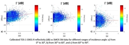
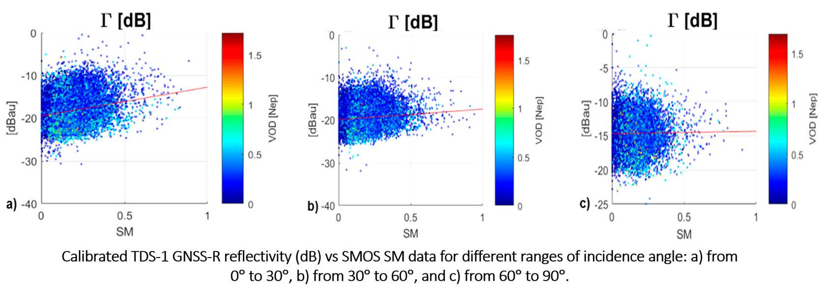
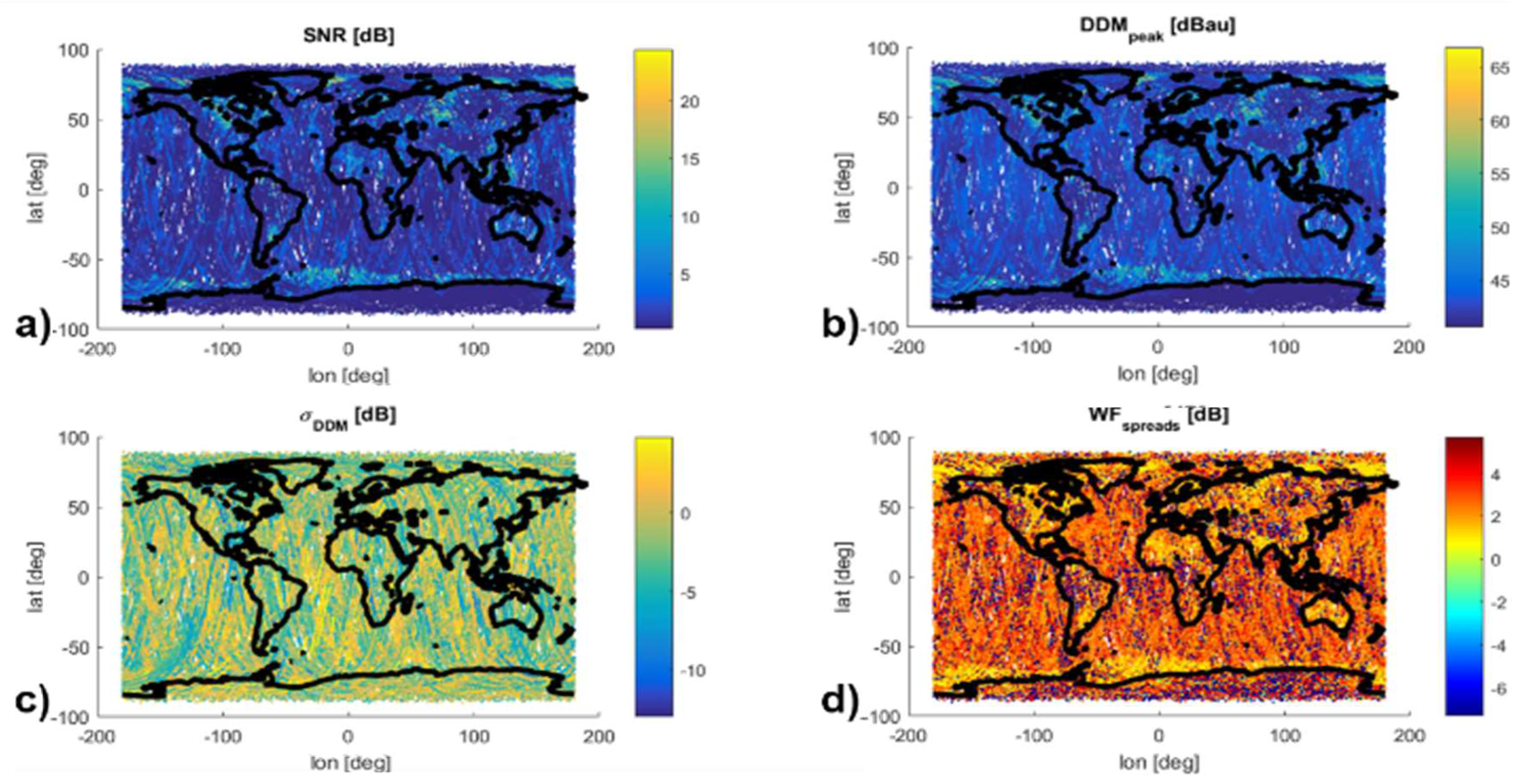
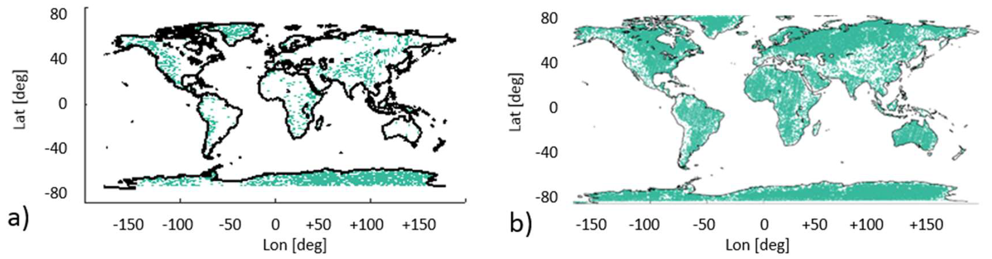
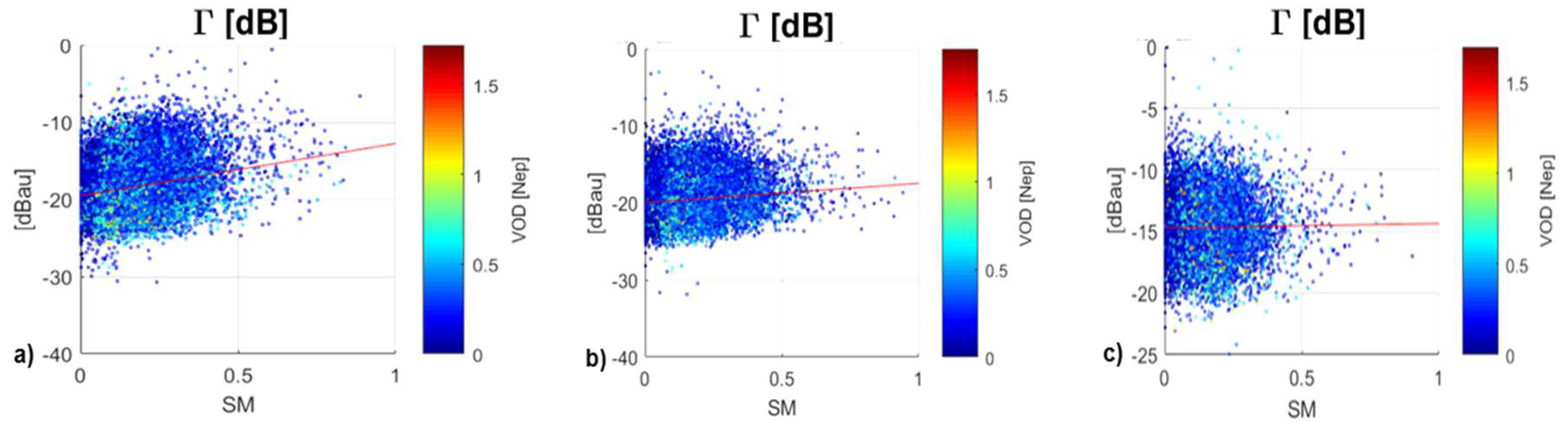
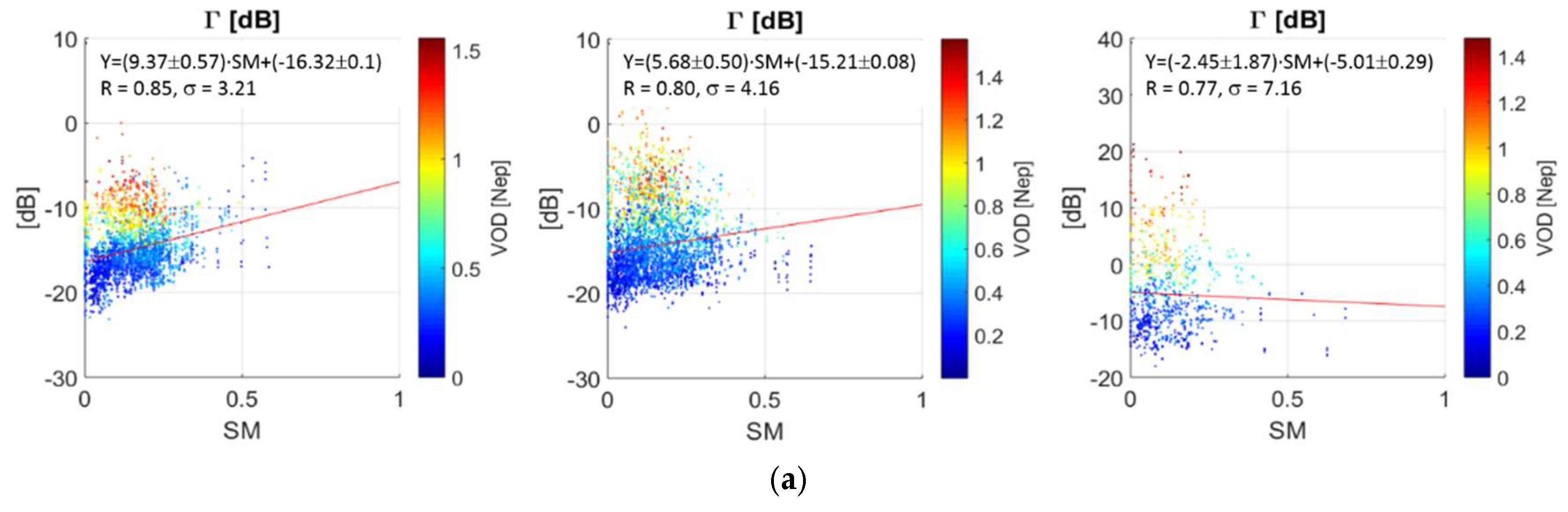
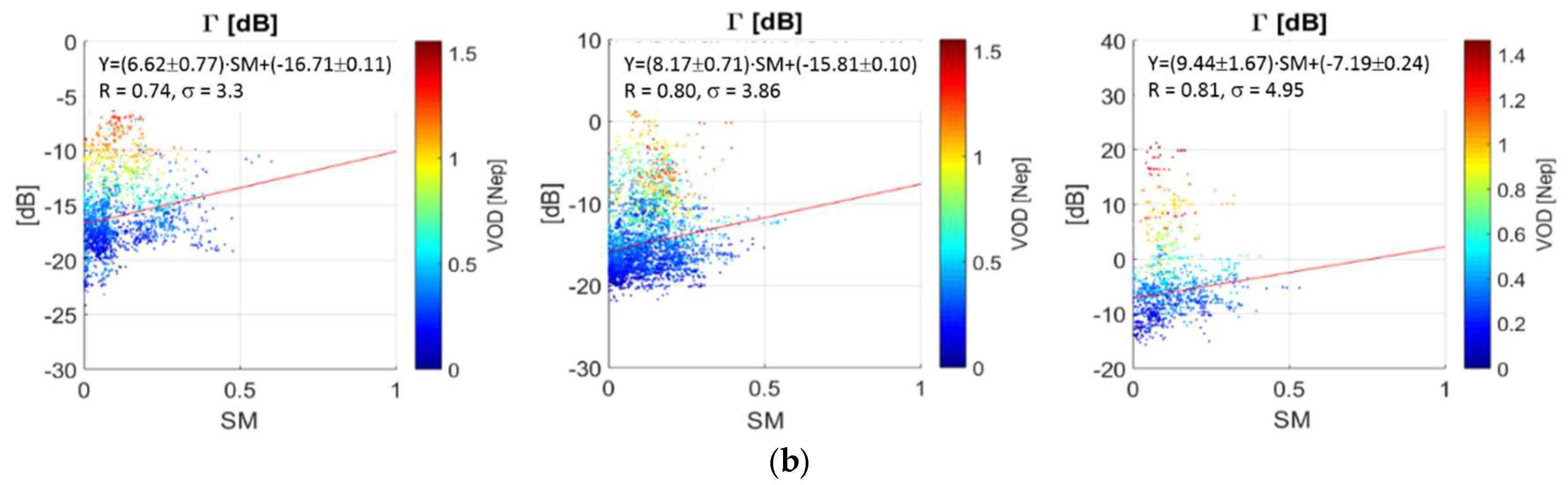
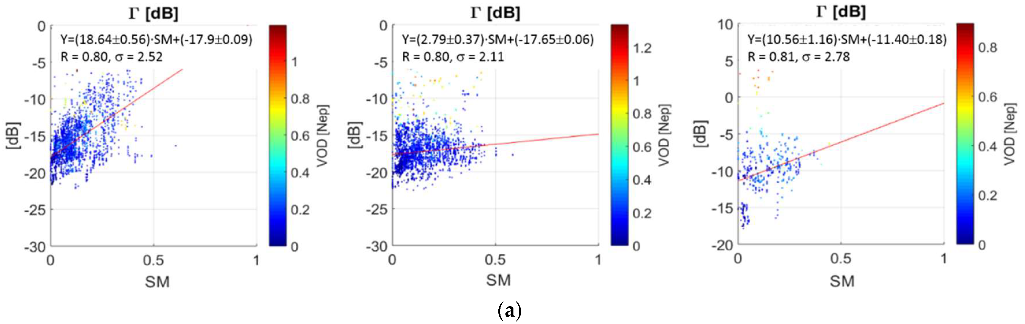
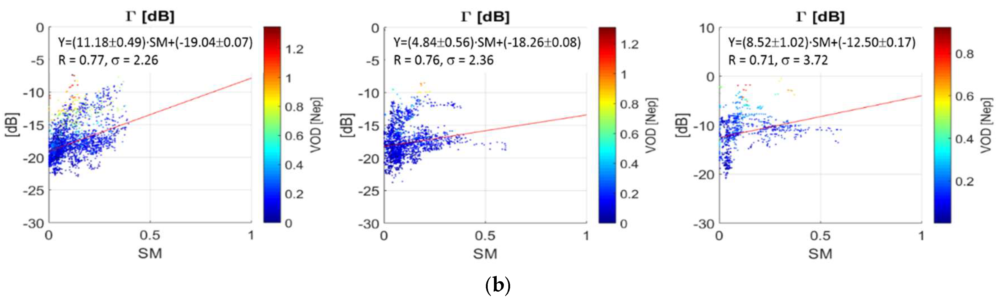
3.1. TDS-1 Data Analysis on a Global Scale

After the TDS-1 data has been quality screened and compensated for all the above effects, different GNSS-R observables are first analyzed. Figure 11 shows the scatter plots of the: (a) SNR; (b) DDM peak; and (c) reflectivity compensated by the distance factor corresponding to incidence angles up to 30° only, vs. the collocated SMOS SM (low-resolution, L3 product, descending pass (no differences have been found if using the ascending or the descending SMOS passes). Note that units are arbitrary (in dB), as it aims only to see which parameters exhibit the largest sensitivity and the lowest error. The color scale shows the VOD in Nepers (Nep). In these scatter plots, the largest values (1.6 Nep) correspond to one-way attenuations of up to ~7 dB. Note that the pixels with the highest VOD are well above the robust fit [27], which suggests that the vegetation scattering effects must be properly taken into account, and that the VOD compensation of Equation (2) may be overcompensating these effects [8]. This effect is more noticeable in the SNR and DDM peak plots, than in the reflectivity ones.
As it can be appreciated, the SNR exhibits the largest uncertainty (σ = 7.1 dB) even after the linear robust fit, but also the largest sensitivity to soil moisture 22.75 dB/100%. The peaks of the DDM (not compensated for the background noise) exhibit a very weak sensitivity to SM, as the signal is masked by the speckle noise (dominant when coherent scattering is present). Reflectivity scatter plot (Figure 11c) exhibits a sensitivity to SM of 9.11 dB/100% and an uncertainty of σ = 3.17 dB/100%.
From now on, only the reflectivity will be analyzed (i.e., neither the SNR, nor the DDMpeak). Figure 12 shows the scatter plots of the (calibrated) reflectivity for incidence angles (a) from 0° to 30°, (b) from 30° to 60°, and (c) from 60° to 90° vs. the collocated SMOS SM.
As it can be appreciated in Figure 12, as the incidence angles increases, the sensitivity to SM decreases: 8.7 dB/100% from 0° to 30°, 5.7 dB/100% from 30° to 60°, and 2.8 dB/100% from 60° to 90°, while the pixels more affected by dense vegetation (large VOD) depart more from the linear robust fit as vegetation effects (multiple scattering and increased attenuation) become more important. Table 2 shows the sensitivities and associated uncertainties estimated using different corrections.
While the obtained values are lower than the ones obtained in previous studies [1,2], they are still significant ~8.75 dB/100% (~0.0875 dB/%). However, the large scattering that remains in the data prevents (so far) from performing an accurate SM retrieval. Part of this scattering is due to the lack of an accurate characterization of the platform attitude an antenna pattern variations in the estimated Pdir, part to the different spatial resolution of the different variables used, part to the pixel inhomogeneity, and part to speckle and thermal noises.
Trying to partially address these issues in the next section a study is conducted to assess the sensitivity to SM using downscaled SMOS products [13,14] and in situ data from CEMADEM (Brazil) [15].

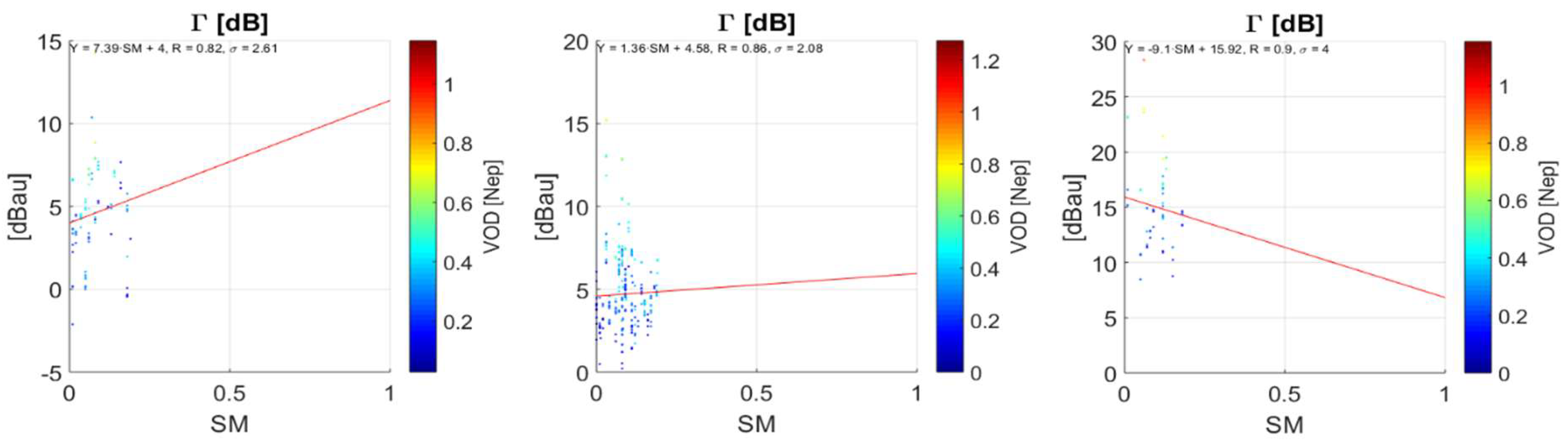
3.2. TDS-1 Data Analysis at Regional Scale

In this section, an analysis similar to the one conducted in the previous section is performed, but over three different regions where 1 km resolution L4 downscaled SMOS surface soil moisture data has been computed. These regions belong to soil moisture networks, and for one of them the LISFLOOD and MUSA hydrological models have been run to estimate the 50 cm and 100 cm SM values, respectively. In practice, TDS-1 GNSS-R ground tracks are so far away from the network stations that few matchups are available, and only when the maximum distance is increased up to 30 km results become statistically significant. Unfortunately, this distance is similar to the SMOS L3 resolution, so no conclusive results can be derived. A description of the different data sets is given below.

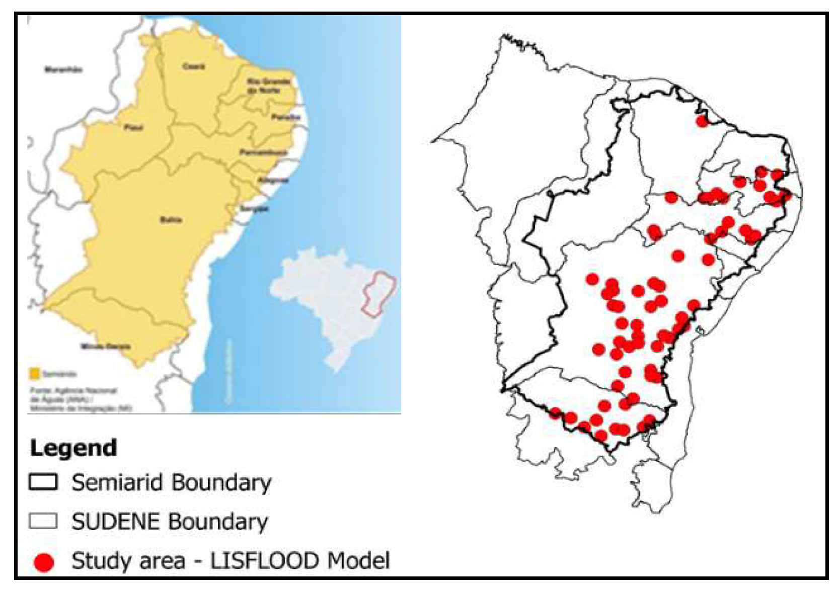
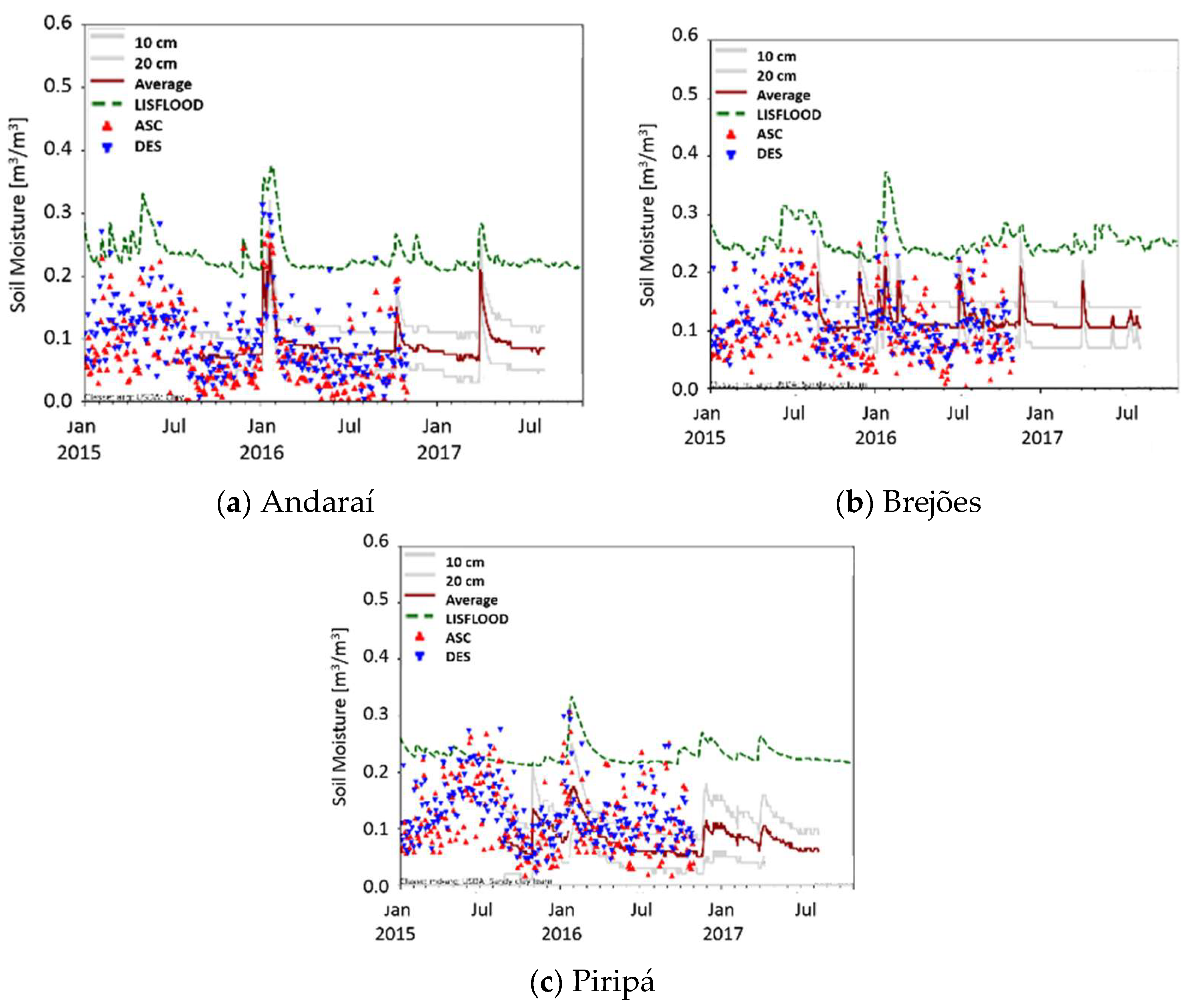
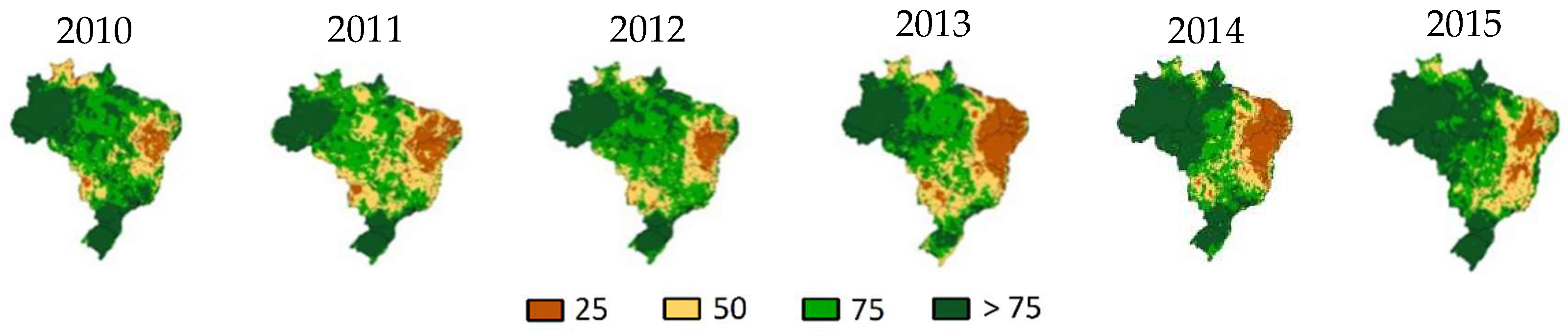
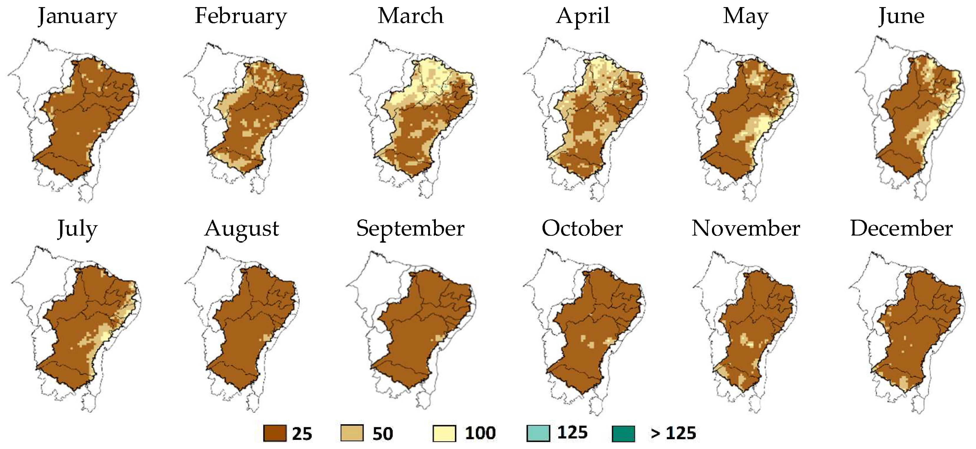
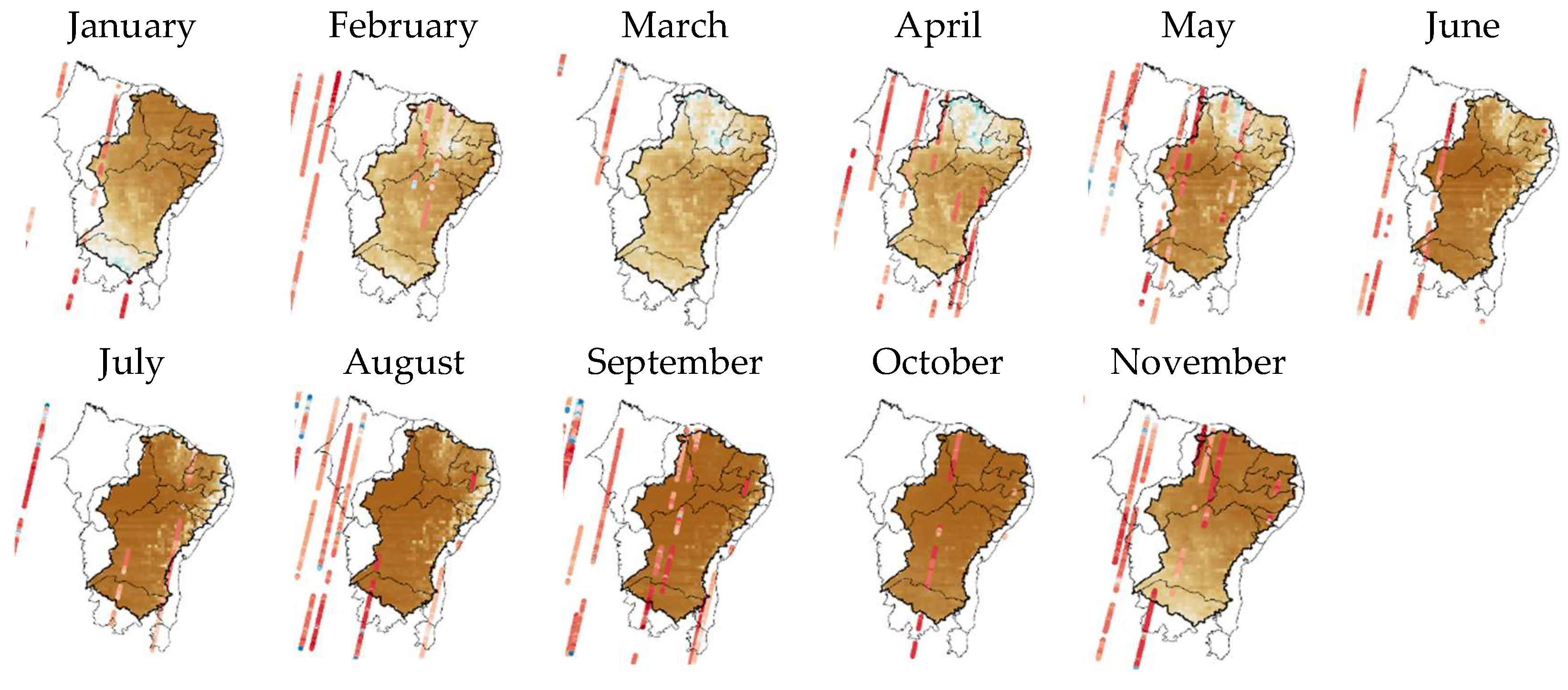
3.2.1. CEMADEM-Brazil

SMOS L3 SM Sensitivity

The area of Brazil analyzed spans from 5° to 25° South, 55° to 25° West. Following the same approach as in Section 3.1, the sensitivity of TDS-1 derived reflection coefficients with respect to SMOS L3 SM data have been derived. Figure 13a shows the main results, when all corrections are applied, and for different ranges of incidence angles. See figure caption for details. Results are discussed at the end.

SMOS L4 SM Sensitivity

Similarly, Figure 13b shows the main results, when all corrections are applied, and for different ranges of incidence angles for SMOS L4 SM (1 km resolution). See figure caption for details. The results will be discussed at the end.

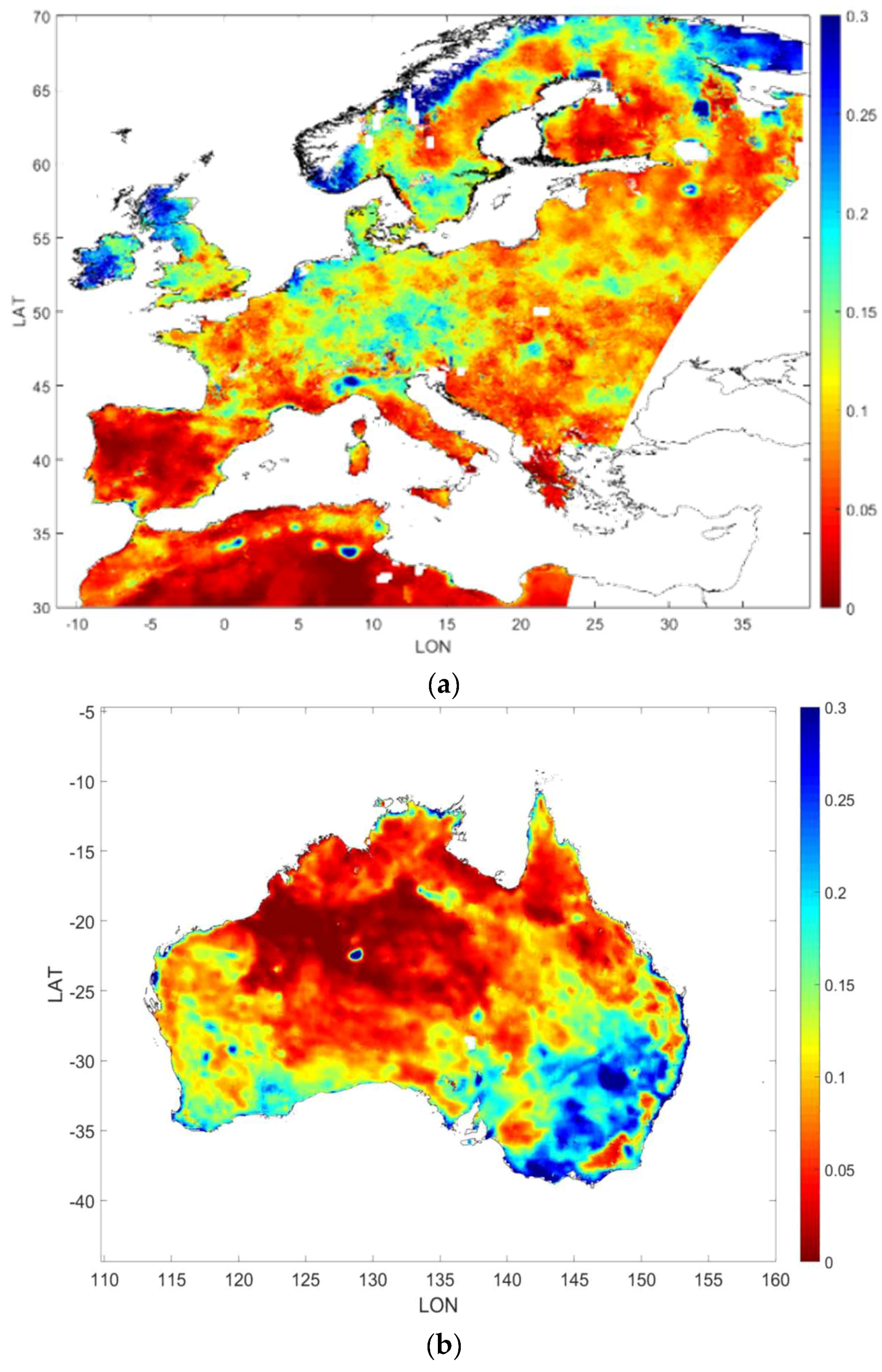
3.2.2. Iberian Peninsula

In order to increase the number of matchups, the whole Iberian Peninsula has been analyzed, i.e., a box from 34° to 45° North, and from 11° West to 5° East. As in Brazil, the sensitivity of the TDS-1 derived GNSS-R reflectivity with respect to the L3 and L4 SMOS SM has been analyzed. Results have been processed separately and are shown below. Note that in these scatter plots, the number of points is relatively much smaller than over Brazil or over Yanco.

SMOS L3 SM Sensitivity

Figure 14a together with Table 3 show the derived sensitivities (slope) to soil moisture. Results have been separated depending on the incidence angle range (0°–30°, 30°–60°, and 60°–90°). Figure 14a shows the main results when all different corrections are applied (vegetation and roughness corrections). These results have been obtained for the period ranging from June 2016 to June 2017. In general, it can be appreciated that higher values of VOD are located at the top of the graphs. This is probably due to an overcorrection of the vegetation effects. This dependence with the vegetation becomes more evident for higher incidence angles as the cosine of the incidence angle tends to zero. Without any kind of correction, the values of the slope are 6.22, 8.94, and −3.87 dB/100%, for the incidence angles from 0° to 30°, from 30° to 60°, and from 60° to 90°, respectively. These same values after applying the vegetation and roughness correction are: 12.15, 11.73, and 22.61 dB/100%, although this last value is unreliable.

SMOS L4 SM Sensitivity

Similarly, Figure 14b shows the main results, when different types of corrections are applied, and for different ranges of incidence angles for SMOS L4 SM (1 km resolution). See figure caption for details. Results will be discussed at the end.

3.2.3. Yanco/NSW/Australia

The New South Wales region in Australia, from −39.45° to −28.39° South, and from 155° to 140° West, has also been studied. As in the previous cases, it has been analyzed the SMOS L3/L4 SM sensitivity with respect to the TDS-1 derived GNSS-R reflectivity. Although for this area the VOD values are lower than in the Iberian Peninsula, the scattering is still significant. In general, the higher slope values are obtained for the incidence angles between 0° and 30° when the vegetation correction is applied.

SMOS L3 SM Sensitivity

Figure 15a shows the main results, when different types of corrections are applied, and for different ranges of incidence angles for SMOS L3 SM (25 km gridded resolution).

SMOS L4 SM Sensitivity

Similarly, Figure 15b shows the main results, when all corrections are applied, and for different ranges of incidence angles for SMOS L4 SM (1 km resolution). See figure caption for details. Results will be discussed at the end.
The graphical results obtained in the previous Sections are now summarized and discussed. Table 3 shows the sensitivities of the TDS-1 GNSS-R reflectivity to the descending-pass SMOS Soil Moisture both for low (25 km) and high resolution (1 km), and for different levels of corrections. Table 4 shows the corresponding number of points used in the regressions.
This suggests that sensitivity is higher over large, relatively flat areas, with low vegetation (e.g., Australia), but as the topography effects and/or vegetation effects increase, this sensitivity decreases, although pixels affected by topography are flagged and discarded, and vegetation effects have been —in principle—compensated for. In any case, all these sensitivities are much smaller than the ones obtained in [1,2], ~38 dB/100%, but it has to be noted that these sensitivities where derived using the SNR as variable, and not the calibrated reflection coefficient, and also, the standard deviation when using the SNR, was almost twice larger than when using the reflections coefficient.

3.3. TDS-1 Data Analysis Using In-situ Soil Moisture Data

When trying to correlate the TDS-1 GNSS-R reflectivity measurements with in situ soil moisture values, very few matchups exist, to the point that it is difficult to perform a robust fit over the Remedhus (Spain) and Yanco (NSW, Australia) sites. Only over Brazil, and taking a 30 km radius, enough matchups have been found to obtain representative results. Results are shown in Figure 16. Sensitivities are 7.39 dB/100%, 1.36 dB/100%, and −9.10 dB/100% for incidence angles from 0° to 30°, from 30° to 60°, and from 60° to 90°, respectively. For incidence angles from 0° to 30°, the value obtained is nicely between 6.62 dB/100% and 9.37 dB/100% encountered in Section 3.2 with respect to L4 and L3 SMOS SM data, respectively. For incidence angles from 60° to 90°, the derived sensitivity to SM is negative, which can be probably attributed to the small number of samples used and the reduced SM range.

3.4. TDS-1 Data Analysis Using Hydrological Models

Considering these results, the sensitivity of the TDS-1 reflectivity and the modelled root zone soil moisture has been analyzed in the Brazilian semiarid region, hoping to encounter a relation such as the one in Lybia desert (Figure 11, [2]). Figure 17 shows a sample scatter plot of the 50 cm LISFLOOD soil moisture and the TDS-1 GNSS-R reflectivity (including surface roughness and vegetation corrections). As it can be appreciated, there is a lot of scatter, but the robust fit derived sensitivity shows a significant sensitivity to the 50 cm depth soil moisture, as large as 12.21 dB/100%, which suggests that in very dry conditions, GNSS-R observables exhibit some sensitivity to the soil moisture at deeper levels.
At first glance, it can be observed that the 1 m depth MUSA soil moisture is not directly correlated with TDS-1 reflectivity. Figure 17 shows the scatter plot between these two variables, showing less significant sensitivity to the soil moisture derived from LISFLOOD. Probably this result is the consequence of the different spatial resolution between models. MUSA model has 25 km, which leaves the soil moisture data more constant when compared to the LISFLOOD model (10 km), and to the fact that MUSA SM is a 100 cm depth, instead of 50 cm.

4. Discussion

On a global scale, the derived GNSS-R reflectivity sensitivity is 8.75 dB/100% using SMOS L3 SM data after applying all corrections (vegetation, surface roughness, topography flag etc.). In the three regions analyzed by using the same SMOS L3 SM values, the sensitivities are significantly higher: 18.64 dB/100% in Yanco/NSW/Australia; 9.37 dB/100% in Cemadem/Brazil; and 12.15 dB/100% over the Iberian Peninsula. They decrease when using SMOS L4 SM data: 11.18 dB/100% in Yanco/NSW/Australia; 6.62 dB/100% in Cemadem/Brazil; and −1.1 dB/100% in the Iberian Peninsula, although this last result is probably not significant because of the limited amount of data, and limited range of SM values. The sensitivities derived in the Brazilian semi-arid region from point measurements are ~7.39 dB/100%, halfway between the values obtained using SMOS L4 and L3 SM values. This variability suggests that the average sensitivity of GNSS-R reflectivity to SM is likely to be close to ~9 dB/100%, but that large uncertainties can be expected regionally, which precludes the need to develop regional soil moisture retrieval algorithms from GNSS-R data.
The sensitivity of GNSS-R reflectivity to subsurface soil moisture has also been analyzed using the LISFLOOD and MUSA models, but the values obtained (12.2 and 49.2 dB/100%) exhibit too low a correlation and are not reliable.

5. Conclusions

A detailed study of the sensitivity of TDS-1 GNSS-R observables vs. SM has been conducted. First, different observables have been examined to understand their potential to infer geophysical data and their problems (e.g., non-geophysical noise, inconsistencies, etc.). Then, the data has been screened for quality and topography effects, compensated for antenna pattern, distance factor, vegetation opacity, and incidence angle. Finally, the sensitivity to SM has been evaluated by a linear robust fit of the scatter plots of the TDS-1 GNSS-R reflectivity with the collocated SMOS SM. While the obtained values are lower than the ones obtained in previous studies [1,2], they are still significant ~9 dB/100% for incidence angles smaller than 30°. However, the large scattering that remains in the data prevents from performing an accurate SM retrieval. Part of this scattering is due to the variations in the estimated direct power, part to the different spatial resolution of the different variables used, part to the pixel inhomogeneity, and part to speckle and thermal noises. In this sense, further studies will be conducted to assess the sensitivity to SM using downscaled SMOS products [13,14] and in situ data from CEMADEM (Brazil) [15].

Author Contributions

Research idea, A.C., M.V.; software coding, A.C., G.P., and L.R.; formal analysis and investigation, A.C., M.V., G.P., and L.R.; data curation, M.V.; writing—original draft preparation, A.C.; writing—review and editing, M.V. and H.P., supervision, A.C.; project administration, A.C.; funding acquisition, A.C., M.V., and H.P.

Funding

This research has been supported by ESA/ESTEC CONTRACT n. 4000120299/17/NL/AF/hh “Potential of spaceborne GNSS-R for land applications”, by project AGORA (ESP2015-70014-C2-1-R) of the Spanish Ministry of Economy and Competitiveness, and by an ICREA Academia Award from the Catalan Government.

Acknowledgments

The authors are thankful to Fabiano Costantini from Deimos-Space for providing the TDS-1 data sets within the framework of the project. The authors are also thankful to N. Pierdicca and L. Guerriero (U. Tor Vergata, Rome, Italy), M. Zribi (CESBIO, Toulouse, France), and M. P. Clarizia (Deimos UK) for the helpful discussions during the execution of this project.

Conflicts of Interest

The authors declare no conflict of interest.

References

  1. Chew, C.; Shah, R.; Zuffada, C.; Hajj, G.; Masters, D.; Mannucci, A.J. Demonstrating soil moisture remote sensing with observations from the UK TechDemoSat-1 satellite mission. Geophys. Res. Lett. 2016, 43, 3317–3324. [Google Scholar] [CrossRef]
  2. Camps, A.; Park, H.; Pablos, M.; Foti, G.; Gommenginger, C.P.; Liu, P.; Judge, J. Sensitivity of GNSS-R Spaceborne Observations to Soil Moisture and Vegetation. IEEE J. Sel. Top. Appl. Earth Obs. Remote Sens. 2016, 9, 4730–4742. [Google Scholar] [CrossRef] [Green Version]
  3. Chew, C.; Small, E.E. Soil Moisture sensing using spaceborne GNSS reflections: Comparison of CYGNSS reflectivity to SMAP soil moisture. Geophys. Res. Lett. 2018, 45, 4049–4057. [Google Scholar] [CrossRef]
  4. Carreno-Luengo, H.; Luzi, G.; Crosetto, M. Impact of the Elevation Angle on CYGNSS-R Bistatic Reflectivity as a function of the Effective Surface Roughness Over Land Surfaces. Remote Sens. 2018, 10, 1749. [Google Scholar] [CrossRef]
  5. Zavorotny, V.U.; Gleason, S.; Cardellach, E.; Camps, A. Tutorial on Remote Sensing Using GNSS Bistatic Radar of Opportunity. IEEE Geosci. Remote Sens. Mag. 2014, 2, 8–45. [Google Scholar] [CrossRef] [Green Version]
  6. Foti, G.; Gommenginger, C.; Unwin, M.; Jales, P.; Tye, J.; Roselló, J. An Assessment of Non-geophysical Effects in Spaceborne GNSS Reflectometry Data from the UK TechDemoSat-1 Mission. IEEE J. Sel. Top. Appl. Earth Obs. Remote Sens. 2017, 10, 3418–3429. [Google Scholar] [CrossRef]
  7. Camps, A.; Park, H.; Juan, J.M.; Sanz, J.; González-Casado, G.; Barbosa, J.; Fabbro, V.; Lemorton, J.; Orús, R. Ionospheric Scintillation Monitoring Using GNSS-R? In Proceedings of the 2018 IEEE International Geoscience and Remote Sensing Symposium, IGARSS 2018, Valencia, Spain, 23–27 July 2018. [Google Scholar]
  8. Schwank, M.; Naderpour, R.; Mätzler, C. Tau-Omega-and Two-Stream Emission Models used for Passive L-band Retrievals: Application to Close-Range Measurements over a Forest. Remote Sens. 2018, in press. [Google Scholar]
  9. O’Neill, P.; Chan, S. Soil Moisture Active Passive (SMAP) Project Algorithm Theoretical Basis Document SMAP L2 and L3 Radiometer Soil Moisture (Passive) Data Products: L2_SM_P L3_SM_P. Available online: https://nsidc.org/sites/nsidc.org/files/files/data/smap/pdfs/l2&3_sm_p_v4_oct2012.pdf (accessed on 30 September 2018).
  10. Barcelona Expert Center. Remote Sensing Research, Data Distribution and Visualization Services: Land Variables. Available online: http://bec.icm.csic.es/land-datasets/ (accessed on 11 November 2018).
  11. Kerr, Y.H.; Waldteufel, P.; Wigneron, J.P.; Delwart, S.; Cabot, F.; Boutin, J.; Escorihuela, M.J.; Font, J.; Reul, N.; Gruhier, C.; et al. The SMOS Mission: New Tool for Monitoring Key Elements of the Global Water Cycle. Proc. IEEE 2010, 98, 666–687. [Google Scholar] [CrossRef] [Green Version]
  12. Font, J.; Camps, A.; Borges, A.; Martin-Neira, M.; Boutin, J.; Reul, N.; Kerr, Y.H.; Hahne, A.; Mecklenburg, S. SMOS: The Challenging Sea Surface Salinity Measurement from Space. Proc. IEEE 2010, 98, 649–665. [Google Scholar] [CrossRef] [Green Version]
  13. Piles, M.; Sánchez, N.; Vall-llossera, M.; Camps, A.; Martínez-Fernández, J.; Martínez, J.; González-Gambau, V. A Downscaling Approach for SMOS Land Observations: Evaluation of High-Resolution Soil Moisture Maps Over the Iberian Peninsula. IEEE J. Sel. Top. Appl. Earth Obs. Remote Sens. 2014, 7, 3845–3857. [Google Scholar] [CrossRef]
  14. Portal, G.; Vall-llossera, M.; Piles, M.; Camps, A.; Chaparro, D.; Pablos, M.; Rossato, L. A Spatially Consistent Downscaling Approach for SMOS Using an Adaptive Moving Window. IEEE J. Sel. Top. Appl. Earth Obs. Remote Sens. 2018, 11, 1883–1894. [Google Scholar] [CrossRef]
  15. Mapa Interativo da Rede Observacional para Monitoramento de Risco de Desastres Naturais do Cemaden. Available online: http://www.cemaden.gov.br/mapainterativo/# (accessed on 2 July 2018).
  16. Celaschi, S.; Xavier, A.L., Jr. Status of a Brazilian Automatic Hydro-meteorological territorial network. In Proceedings of the XXXIV Simpósio Brasileiro de Telecomunicaçoes, SBrT2016, Santarem, Brazil, 30 August–2 September 2016. [Google Scholar]
  17. Du, J.; Kimball, J.S.; Moghaddam, M. Theoretical Modeling and Analysis of L- and P-band Radar Backscatter Sensitivity to Soil Active Layer Dielectric Variations. Remote Sens. 2015, 7, 9450–9472. [Google Scholar] [CrossRef] [Green Version]
  18. Zwieback, S.; Hensley, S.; Hajnsek, I. Assessment of soil moisture effects on L-band radar interferometry. Remote Sens. Environ. 2015, 164, 77–89. [Google Scholar] [CrossRef] [Green Version]
  19. Thornthwaite, C.W.; Mather, J.R. The Water Balance; Laboratory of Climatology: Centerton, NJ, USA, 1955. [Google Scholar]
  20. Thornthwaite, C.W.; Mather, J.R. Instructions and Tables for Computing Potential Evapotranspiration and the Water Balance. Laboratory in Climatology, Drexel Institute of Technology: Philadelphia, PA, USA, 1957; Volume 10, pp. 185–311. [Google Scholar]
  21. Burek, P.; van der Knijff, J.M.; de Roo, A. LISFLOOD—Distributed Water Balance and flood Simulation Model—Revised User Manual; 2013. Available online: http://publications.jrc.ec.europa.eu/repository/bitstream/JRC78917/lisflood_2013_online.pdf (accessed on 16 November 2018).
  22. Monitoramento de Umidade do Solo no Sudeste da América do Sul. Available online: http://musa.cptec.inpe.br/ (accessed on 2 July 2018).
  23. Doyle, M.E.; Tomasella, J.; Rodriguez, D.A.; Chou, S.C. Experiments using new initial soil moisture conditions and soil map in the Eta model over La Plata Basin. Meteorol. Atmos. Phys. 2013, 121, 119–136. [Google Scholar] [CrossRef] [Green Version]
  24. Marengo, J.A.; Torres, R.R.; Alves, L.M. Drought in Northeast Brazil—Past, present, and future. Theor. Appl. Clim. 2016, 20, 1189–1200. [Google Scholar] [CrossRef]
  25. Holland, P.W.; Welsch, R.E. Robust Regression Using Iteratively Reweighted Least-Squares. Commun. Stat. Theory Methods 1977, 6, 813–827. [Google Scholar] [CrossRef]
  26. Rossato, L.; Marengo, J.A.; de Angelis, C.F.; Pires, L.B.M.; Mendiondo, E.M. Impact of soil moisture over Palmer Drought Severity Index and its future projections in Brazil. RBRH 2017, 22, e36. [Google Scholar] [CrossRef]
  27. Rossato, L.; Vall-llossera, M.; Camps, A.; Piles, M.; Portal, G.; Chaparro, D.; Alvalá, R. Validation of the SMOS-BEC products in different networks. In Proceedings of the Satellite Soil Moisture Validation and Application Workshop, Wien, Austria, 19–20 September 2017; Available online: http://smw.geo.tuwien.ac.at/abstract-booklet (accessed on 16 November 2018).
Figure 1. Sample TechDemoSat-1 (TDS-1) data: (a) SNR [dB] computed as the ratio of the peak of the Delay Doppler Maps (DDM) to the noise; (b) DDM peak; (c) standard deviation of the peak; and (d) waveform spread figure of merit.
Remotesensing 10 01856 g001
Figure 2. pdf’s of the DDM spread parameters over land only: (a) delay (units = 0.25 × C/A chips) and (b) Doppler frequency (units = 500 Hz bins).
Remotesensing 10 01856 g002
Figure 3. (a) Pixels corresponding to different ranges of DDM delay spread (στ) and DDM Doppler frequency spread ( σ f d ) parameters. (b) Surface topography flag derived from a Digital Elevation Model. White pixels correspond to pixels that may be affected by topography. Note that it is nearly the negative of Figure 3a.
Remotesensing 10 01856 g003
Figure 4. Antenna pattern as a function of the incidence angle.
Remotesensing 10 01856 g004
Figure 5. Sample 1 km L4 downscaled average SM maps over (a) Europe (6/2011), and (b) Australia (6/2015).
Remotesensing 10 01856 g005
Figure 6. Map of Brazil showing the location of some of the CEMADEN in situ stations [16].
Remotesensing 10 01856 g006
Figure 7. Sample temporal series of SM obtained from CEMADEN stations (10 and 20 cm, gray lines; average value: red solid line), LISFLOOD model (50 cm depth, green line), SMOS L4 products (ascending and descending passes—red and blue line, respectively) during 2015–2016 for different sites located in Bahia (Brazilian Semiarid region). Sites selected to exhibit different correlation values with ascending-pass SMOS SM data.
Remotesensing 10 01856 g007
Figure 8. Yearly average spatial-temporal distribution of the soil water storage [mm] derived from MUSA model at 1 m depth in the Brazilian semiarid during representative years 2010 to 2015.
Remotesensing 10 01856 g008
Figure 9. Monthly average spatial-temporal distribution of the soil water storage [mm] derived from MUSA model at 1 m depth in the Brazilian semiarid during 2015.
Remotesensing 10 01856 g009
Figure 10. Monthly average spatial-temporal distribution of soil moisture (mm) derived from MUSA model during 2015 year (January to November) and TDS-1 GNSS-R reflectivity (all incidence angles).
Remotesensing 10 01856 g010
Figure 11. Screened and compensated TDS-1 GNSS-R observables vs. SMOS SM data: (a) SNR [dB], (b) DDMpeak [dB], (c) Г [dB] over θi ≤ 30°.
Remotesensing 10 01856 g011
Figure 12. Calibrated TDS-1 GNSS-R reflectivity Г [dB] but not corrected for vegetation and surface roughness effects vs. SMOS SM data for different ranges of incidence angle: (a) from 0° to 30°; (b) from 30° to 60°; and (c) from 60° to 90°.
Remotesensing 10 01856 g012
Figure 13. Scatter plot between the (a) Low Resolution (25 km) SMOS L3 SM and (b) High Resolution (1 km) SMOS L4 SM and the TDS-1 reflectivity value over the CEMADEM region from June 2016 to June 2017, with vegetation and roughness corrections applied. Each column represents the values for a specific range of incidence angles: (left) 0°–30°; (center) 30°–60°; and (right) 60°–90°.
Remotesensing 10 01856 g013aRemotesensing 10 01856 g013b
Figure 14. Scatter plot between the (a) Low Resolution (25 km) SMOS L3 SM and (b) High Resolution (1 km) SMOS L4 SM and the TDS-1 reflectivity value over the Iberian Peninsula from June 2016 to June 2017, with vegetation and roughness corrections applied. Each column represents the values for a specific range of incidence angles: (left) 0°–30°; (center) 30°–60°; and (right) 60°–90°.
Remotesensing 10 01856 g014
Figure 15. Scatter plot between the (a) Low Resolution (25 km) SMOS L3 SM and (b) High Resolution (1 km) SMOS L4 SM and the TDS-1 reflectivity value over Yanco/NSW/Australia from June 2016 to June 2017, with vegetation and roughness corrections applied. Each column represents the values for a specific range of incidence angles: (left) 0°–30°; (center) 30°–60°; and (right) 60°–90°.
Remotesensing 10 01856 g015aRemotesensing 10 01856 g015b
Figure 16. Same as Figure 16, but over CEMADEM/Brazil, using a radius of ~30 km from the soil moisture stations. Note the limited range of Soil Moisture values, as this region corresponds to the so-called Brazilian semi-arid.
Remotesensing 10 01856 g016
Figure 17. Scatter plot TDS-1 GNSS-R reflectivity (all corrections included) and (a) 50 cm depth LISFLOOD soil moisture [m3/m3] for Andaraí station, and (b) 1 m depth MUSA soil moisture for 2015.
Remotesensing 10 01856 g017
Table 1. Correlation between CEMADEM stations SM at 10 cm and SMOS L4 SM and LISFLOOD model at the ascending or descending satellite passes. In boldface: stations with correlation smaller than 0.5.
CEMADEN StationsLatitudeLongitudeSMOSLISFLOOD
AscDesAscDes
Abaíra−13.26−41.660.650.580.570.44
Andaraí−12.59−41.010.750.720.70.59
Aracatu−14.45−41.450.750.520.630.52
Barro Alto−11.81−41.900.610.510.590.53
Bom Jesus da Serra−14.38−40.490.650.550.50.39
Brejões−13.10−39.790.470.370.430.44
Cabeceiras do Paraguaçu−12.62−39.230.490.440.50.52
Caldeirão Grande−11.05−40.150.570.310.330.31
Cândido Sales−15.51−41.150.720.620.410.36
Castro Alves−12.75−39.440.530.480.310.3
Dom Basílio−13.75−41.770.640.530.650.46
Ibicoara−13.45−41.300.740.590.510.41
Ipecaetá−12.29−39.320.520.400.390.24
Itaeté−13.03−40.960.630.590.610.53
Jeremoabo−10.00−38.330.150.10.150.11
Jussara−10.96−41.940.690.590.690.59
Lajedo do Tabocal−13.43−40.240.490.360.370.32
Lamarão−11.82−38.870.30.40.380.42
Mundo Novo−11.86−40.480.50.50.510.53
Canarana−14.66−40.270.490.390.370.29
Nova Itarana−13.00−40.010.360.340.350.2
Palmeiras−12.52−41.570.550.560.490.41
Piripá−15.01−41.740.080.10.170.2
Planalto−14.60−40.480.730.660.280.66
São Gabriel−11.22−41.900.50.530.370.3
Table 2. Reflectivity fit with respect to range of incidence angles for different corrections: NO: no vegetation correction, no surface roughness correction; R: no vegetation (VOD, ω) correction, surface roughness correction applied; and V + R: vegetation (VOD, ω = 0) and surface roughness corrections applied.
Г = (a ± Δa)·SM + (b ± Δb)
a Δa b Δb
NORV + RNORV + RNORV + RNORV + R
0° to 30°6.766.478.750.200.200.20−19.52−18.92−16.260.170.170.21
30° to 60°2.472.205.660.100.100.20−19.92−19.32−16.130.120.120.20
60° to 90°0.350.042.780.200.200.50−14.70−14.10−8.220.240.240.54
Table 3. Slopes of the regression lines shown in the Figure 13, Figure 14 and Figure 15, and SMOS L2 SM (Low Resolutions) and SMOS L3 Soil Moisture (High Resolution). Note: NO” stands for no corrections applied, “R” for surface roughness correction applied only, “V” for vegetation corrections applied, and “V + R” for vegetation and surface roughness corrections applied. NO, R, and V cases not presented in Figure 13, Figure 14 and Figure 15.
BRAZILIBERIAN PENINSULAAUSTRALIA
Correct0°–30°30°–60°60°–90°0°–30°30°–60°60°–90°0°–30°30°–60°60°–90°
SMOS L3 SM (25 km)NO3.631.771.376.228.94−3.8715.17−0.163.47
R3.541.621.115.459.08−3.6515.250.033.67
V9.455.84−3.1712.9711.5722.6918.472.6110.39
V + R9.375.68−2.4512.1511.7322.6118.642.7910.56
SMOS L2 SM (1 km)NO2.441.262.67−4.28.632.827.713.665.24
R2.302.551.13−4.468.62.537.993.75.34
V6.728.319.56−0.412.54−6.3510.974.858.4
V + R6.628.179.441.112.51−6.7411.184.848.52
Table 4. Number of points of the regression lines shown in the Figure 13, Figure 14 and Figure 15, and SMOS L2 SM (Low Resolutions) and SMOS L3 Soil Moisture (High Resolution). Note: NO” stands for no corrections applied, “R” for surface roughness correction applied only, “V” for vegetation corrections applied, and “V + R” for vegetation and surface roughness corrections applied. NO, R, and V cases not presented in Figure 13, Figure 14 and Figure 15.
BRAZILIBERIAN PENINSULAAUSTRALIA
Correct0°–30°30°–60°60°–90°0°–30°30°–60°60°–90°0°–30°30°–60°60°–90°
SMOS L3 SM (25 km)NO12,14319,678513217631726505639267521815
R12,10819,649509917331698499639067461815
V44557720174148972320428183295706
V + R44557716174148671920428183295706
SMOS L2 SM (1 km)NO647311,672297724771413335499256161805
R646711,657294513091308368499256101805
V220044191224435385126287127411139
V + R220044171224849552134287127411139

