Improving the Seasonal Representation of ASCAT Soil Moisture and Vegetation Dynamics in a Temperate Climate

 , , , ,
  and
and 
Abstract
1. Introduction
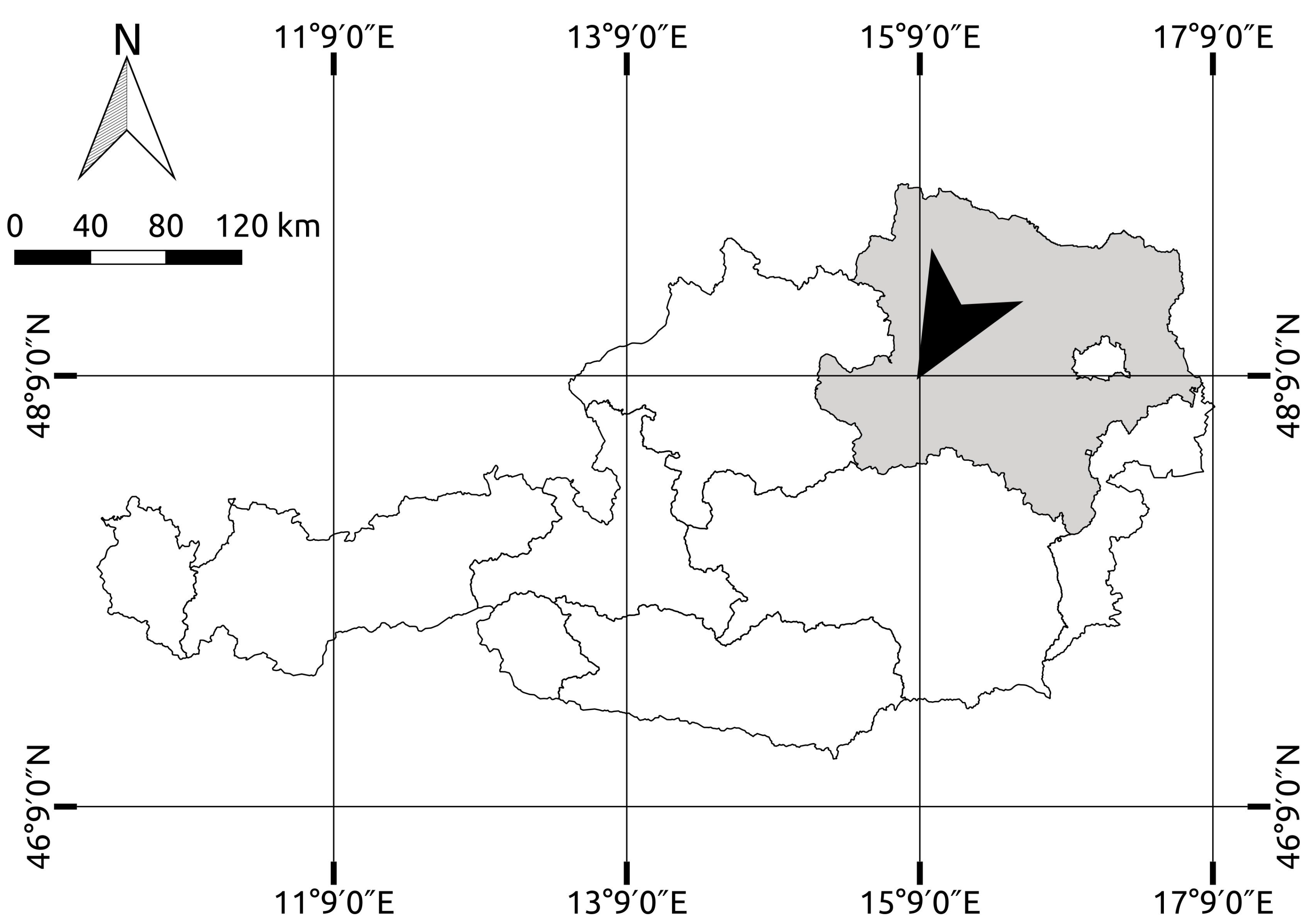
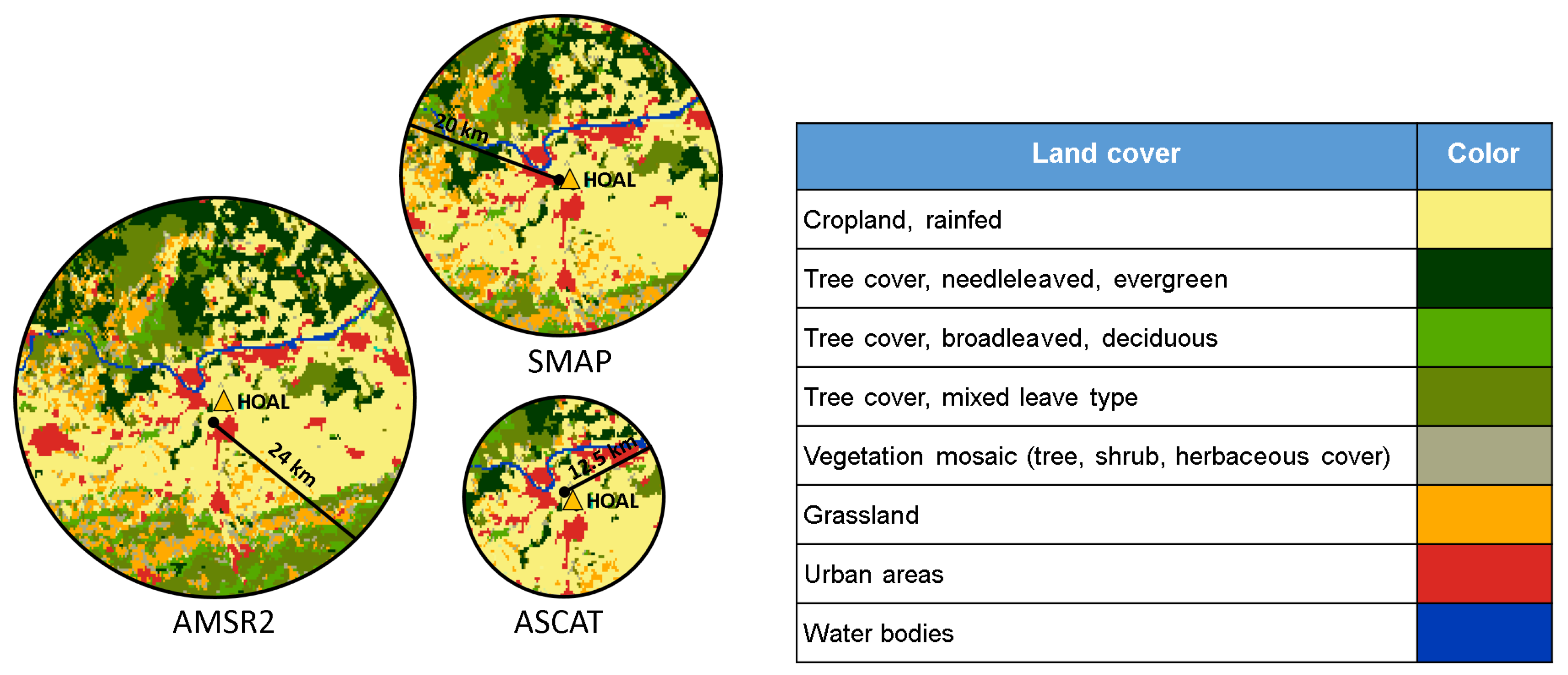
2. Study Site
3. Datasets
3.1. In Situ Soil Moisture
3.2. Satellite Data
3.2.1. ASCAT
3.2.2. AMSR2
3.2.3. SMAP
3.2.4. SPOT-VGT and PROBA-V
3.3. Pre-Processing
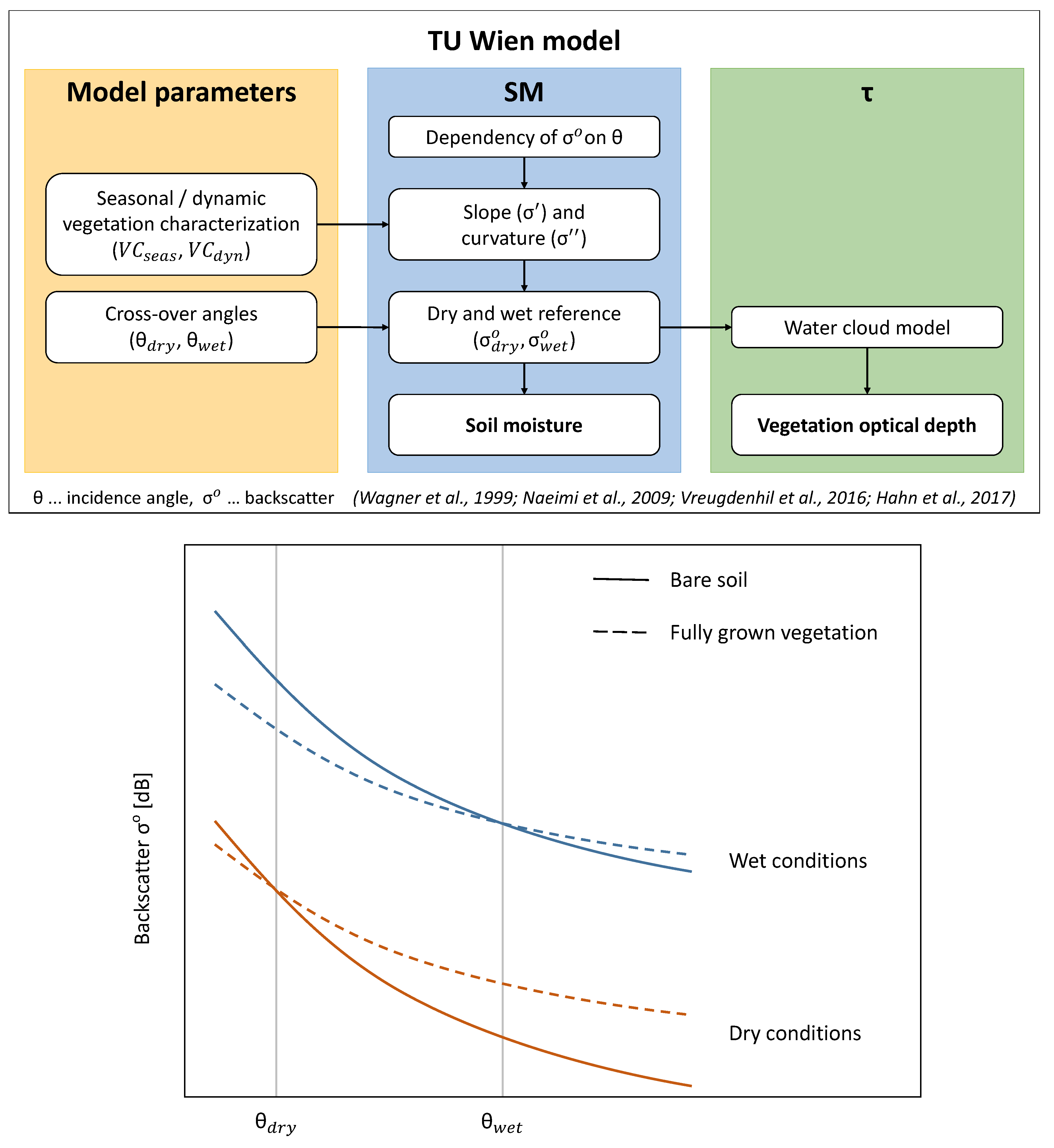
4. Methods
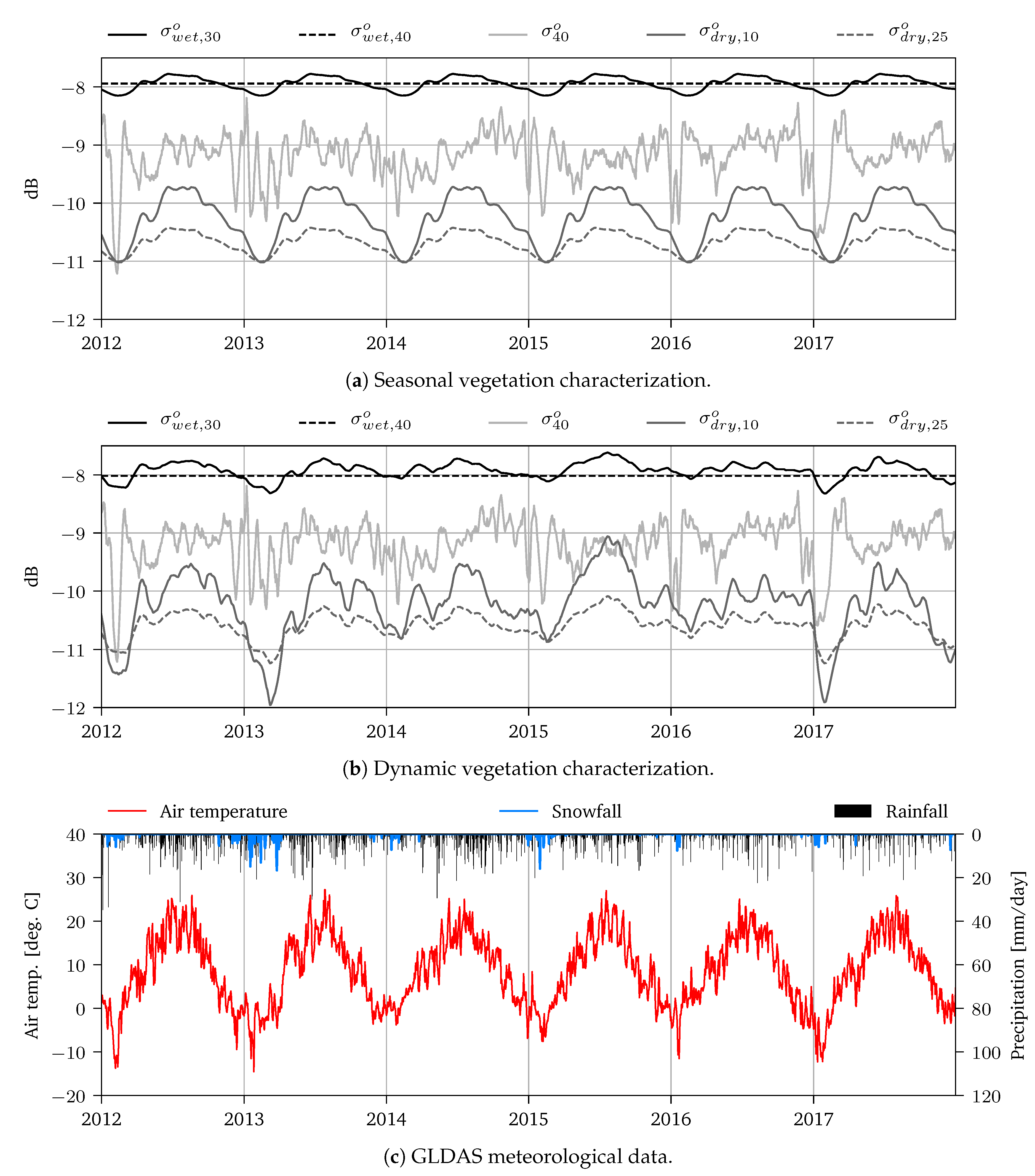
4.1. Type of Vegetation Characterization
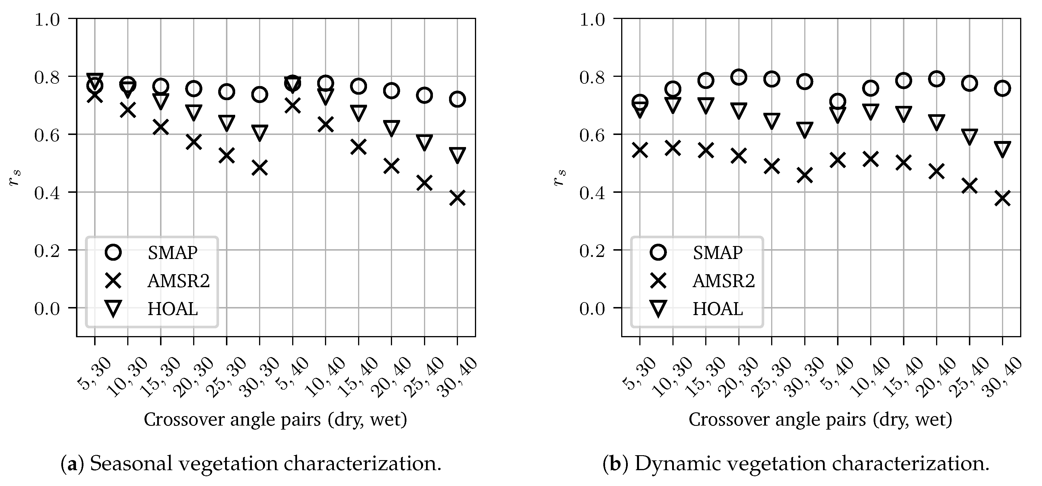
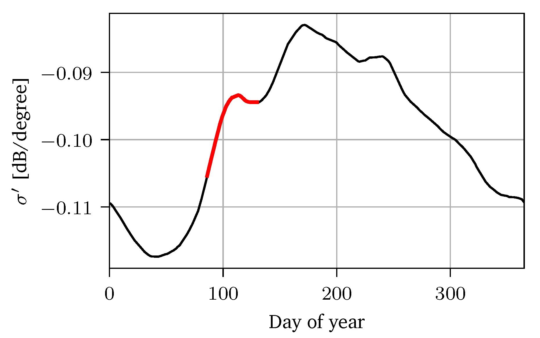
4.2. Selection of Cross-Over Angles
4.3. Evaluation of the Results
5. Results
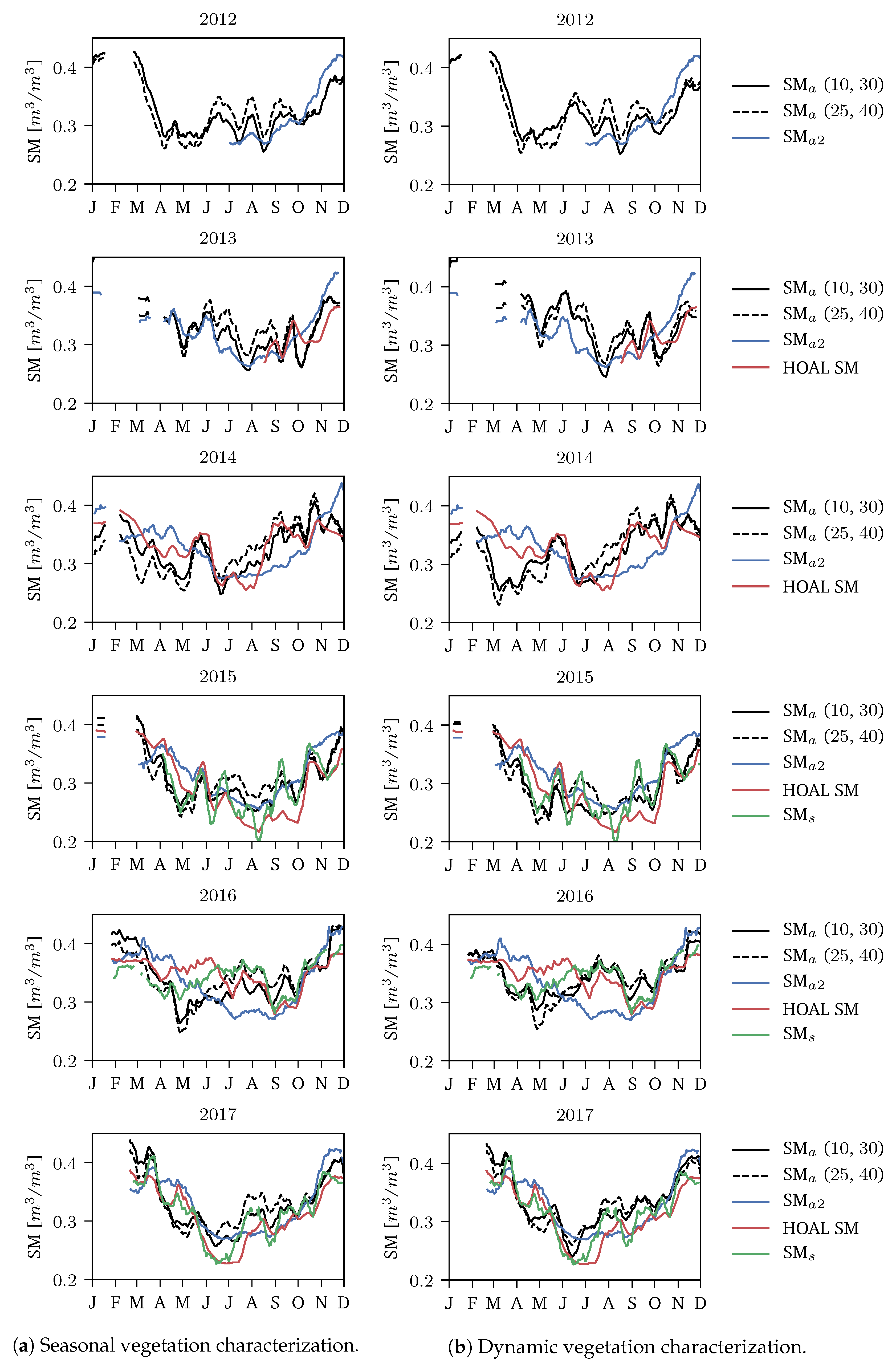
5.1. Soil Moisture
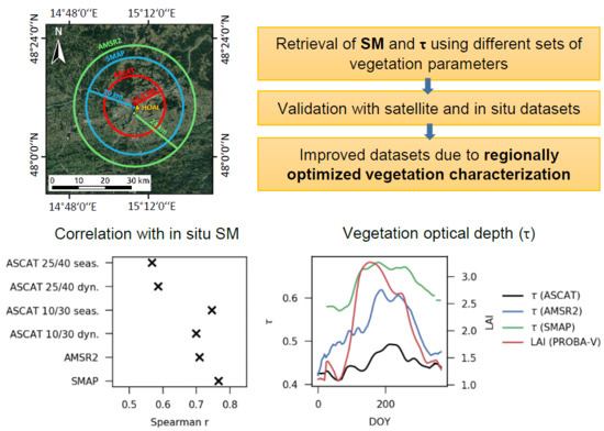
5.1.1. Cross-Over Angle Optimization
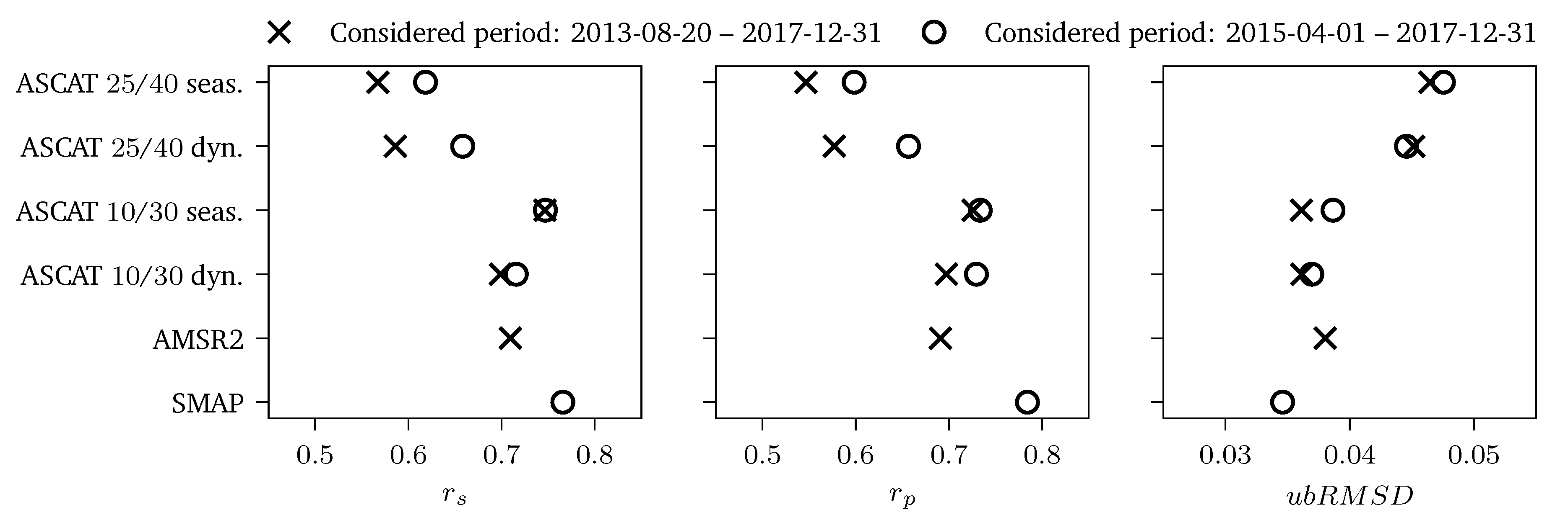
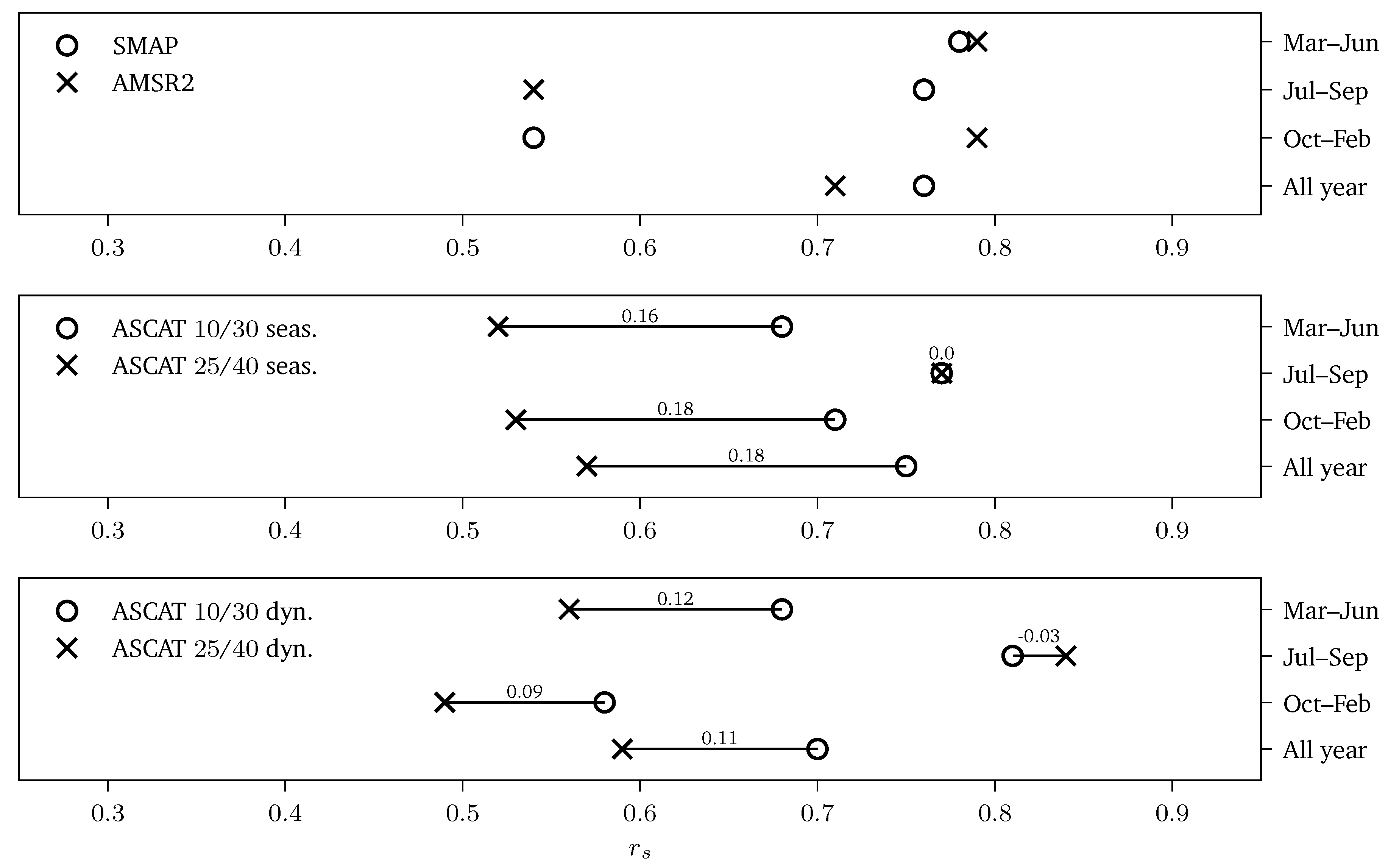
5.1.2. Quantitative Comparison
5.1.3. Qualitative Comparison
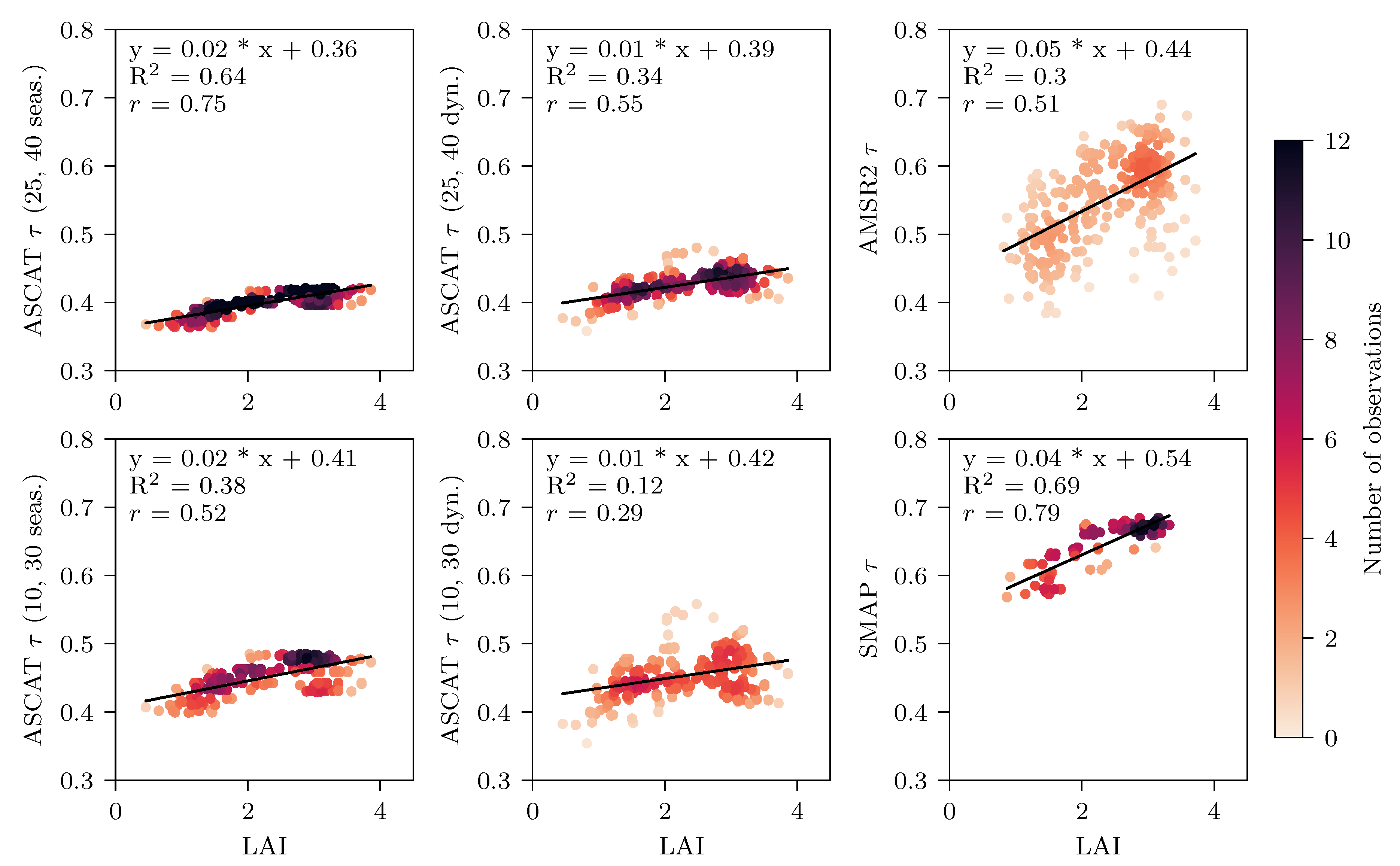
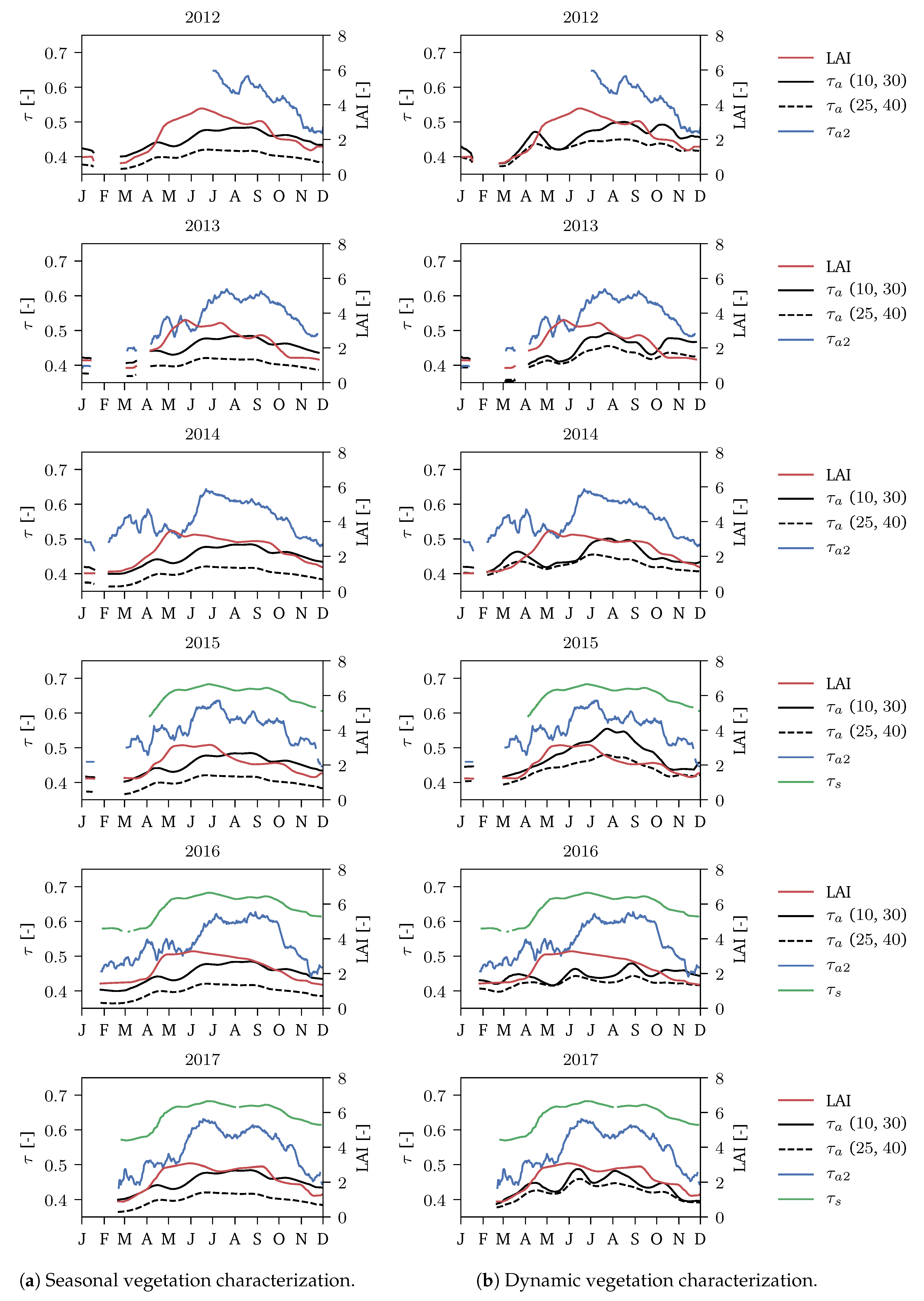
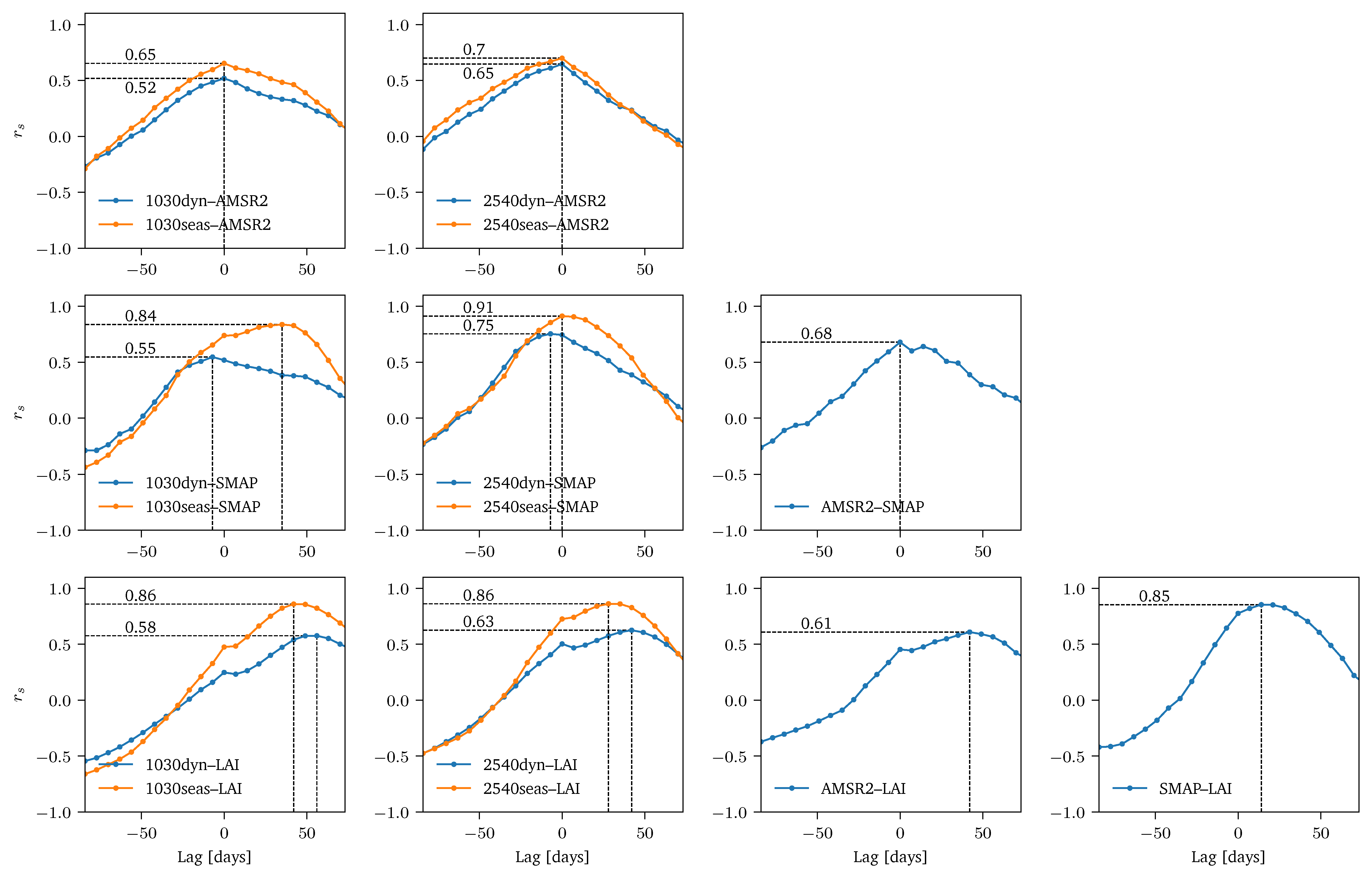
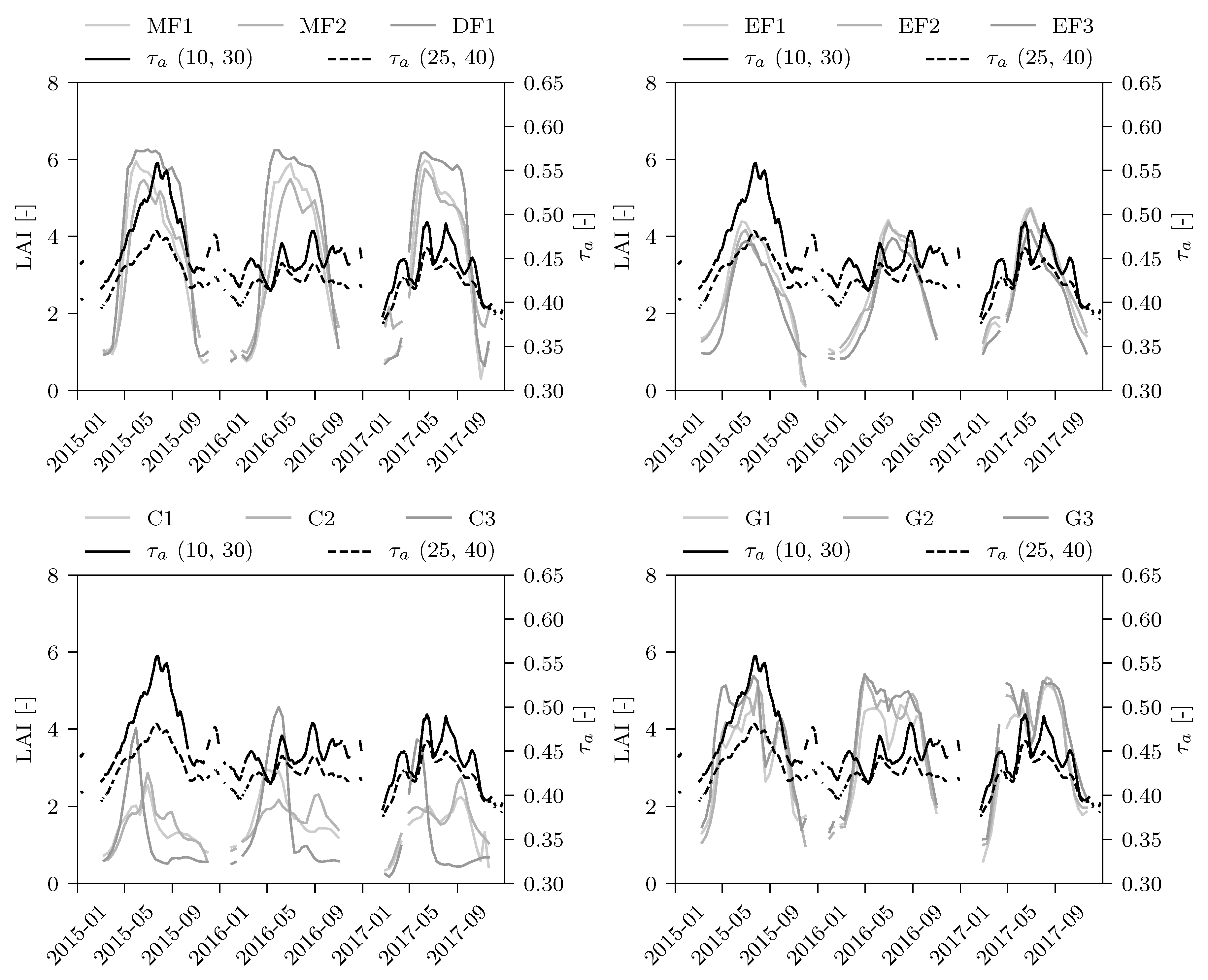
5.2. Vegetation Optical Depth ()
5.2.1. Quantitative Comparison
5.2.2. Qualitative Comparison
5.2.3. Land Cover Effect
6. Discussion
7. Conclusions
Author Contributions
Funding
Acknowledgments
Conflicts of Interest
Abbreviations
| AMSR2 | Advanced Microwave Scanning Radiometer 2 |
| ASCAT | Advanced Scatterometer |
| HOAL | Hydrological Open Air Laboratory |
| LAI | Leaf area index |
| SM | Soil moisture |
| SMAP | Soil Moisture Active Passive |
| Vegetation optical depth | |
| Vegetation characterization using seasonal parameters | |
| Vegetation characterization using dynamic parameters |
References
- Wanders, N.; Bierkens, M.F.; de Jong, S.M.; de Roo, A.; Karssenberg, D. The benefits of using remotely sensed soil moisture in parameter identification of large-scale hydrological models. Water Resour. Res. 2014, 50, 6874–6891. [Google Scholar] [CrossRef]
- Wanders, N.; Karssenberg, D.; Roo, A.D.; De Jong, S.; Bierkens, M. The suitability of remotely sensed soil moisture for improving operational flood forecasting. Hydrol. Earth Syst. Sci. 2014, 18, 2343–2357. [Google Scholar] [CrossRef]
- Brocca, L.; Melone, F.; Moramarco, T.; Wagner, W.; Naeimi, V.; Bartalis, Z.; Hasenauer, S. Improving runoff prediction through the assimilation of the ASCAT soil moisture product. Hydrol. Earth Syst. Sci. 2010, 14, 1881–1893. [Google Scholar] [CrossRef]
- Ling, P. A review of soil moisture sensors. Assn. Flor. Prof. Bull. 2004, 886, 22–23. [Google Scholar]
- Soulis, K.X.; Elmaloglou, S.; Dercas, N. Investigating the effects of soil moisture sensors positioning and accuracy on soil moisture based drip irrigation scheduling systems. Agric. Water Manag. 2015, 148, 258–268. [Google Scholar] [CrossRef]
- Koster, R.D.; Dirmeyer, P.A.; Guo, Z.C.; Bonan, G.; Chan, E.; Cox, P.; Gordon, C.T.; Kanae, S.; Kowalczyk, E.; Lawrence, D.; et al. Regions of strong coupling between soil moisture and precipitation. Science 2004, 305, 1138–1140. [Google Scholar] [CrossRef] [PubMed]
- Brocca, L.; Massari, C.; Ciabatta, L.; Moramarco, T.; Penna, D.; Zuecco, G.; Pianezzola, L.; Borga, M.; Matgen, P.; Martínez-Fernández, J. Rainfall estimation from in situ soil moisture observations at several sites in Europe: An evaluation of the SM2RAIN algorithm. J. Hydrol. Hydromech. 2015, 63, 201–209. [Google Scholar] [CrossRef]
- Svoboda, M.; LeComte, D.; Hayes, M.; Heim, R.; Gleason, K.; Angel, J.; Rippey, B.; Tinker, R.; Palecki, M.; Stooksbury, D.; et al. The drought monitor. Bull. Am. Meteorol. Soc. 2002, 83, 1181–1190. [Google Scholar] [CrossRef]
- Hao, Z.; AghaKouchak, A. A nonparametric multivariate multi-index drought monitoring framework. J. Hydrometeorol. 2014, 15, 89–101. [Google Scholar] [CrossRef]
- Martínez-Fernández, J.; González-Zamora, A.; Sánchez, N.; Gumuzzio, A.; Herrero-Jiménez, C. Satellite soil moisture for agricultural drought monitoring: Assessment of the SMOS derived Soil Water Deficit Index. Remote Sens. Environ. 2016, 177, 277–286. [Google Scholar] [CrossRef]
- Rodell, M.; Velicogna, I.; Famiglietti, J.S. Satellite-based estimates of groundwater depletion in India. Nature 2009, 460, 999. [Google Scholar] [CrossRef] [PubMed]
- Wagner, W.; Hahn, S.; Kidd, R.; Melzer, T.; Bartalis, Z.; Hasenauer, S.; Figa-Saldaña, J.; de Rosnay, P.; Jann, A.; Schneider, S.; et al. The ASCAT soil moisture product: A review of its specifications, validation results, and emerging applications. Meteorol. Z. 2013, 22, 5–33. [Google Scholar] [CrossRef]
- Wagner, W.; Dorigo, W.; de Jeu, R.; Fernandez, D.; Benveniste, J.; Haas, E.; Ertl, M. Fusion of active and passive microwave observations to create an essential climate variable data record on soil moisture. ISPRS Ann. Photogramm. Remote Sens. Spat. Inf. Sci. 2012, 7, 315–321. [Google Scholar]
- Kerr, Y.H.; Waldteufel, P.; Wigneron, J.P.; Martinuzzi, J.; Font, J.; Berger, M. Soil moisture retrieval from space: The Soil Moisture and Ocean Salinity (SMOS) mission. IEEE Trans. Geosci. Remote Sens. 2001, 39, 1729–1735. [Google Scholar] [CrossRef]
- Entekhabi, D.; Njoku, E.G.; O’Neill, P.E.; Kellogg, K.H.; Crow, W.T.; Edelstein, W.N.; Entin, J.K.; Goodman, S.D.; Jackson, T.J.; Johnson, J.; et al. The soil moisture active passive (SMAP) mission. Proc. IEEE 2010, 98, 704–716. [Google Scholar] [CrossRef]
- Parinussa, R.M.; Holmes, T.R.; Wanders, N.; Dorigo, W.A.; de Jeu, R.A. A preliminary study toward consistent soil moisture from AMSR2. J. Hydrometeorol. 2015, 16, 932–947. [Google Scholar] [CrossRef]
- Wagner, W.; Lemoine, G.; Rott, H. A method for estimating soil moisture from ERS scatterometer and soil data. Remote Sens. Environ. 1999, 70, 191–207. [Google Scholar] [CrossRef]
- Naeimi, V.; Scipal, K.; Bartalis, Z.; Hasenauer, S.; Wagner, W. An improved soil moisture retrieval algorithm for ERS and METOP scatterometer observations. IEEE Trans. Geosci. Remote Sens. 2009, 47, 1999–2013. [Google Scholar] [CrossRef]
- Matgen, P.; Heitz, S.; Hasenauer, S.; Hissler, C.; Brocca, L.; Hoffmann, L.; Wagner, W.; Savenije, H. On the potential of MetOp ASCAT-derived soil wetness indices as a new aperture for hydrological monitoring and prediction: A field evaluation over Luxembourg. Hydrol. Process. 2012, 26, 2346–2359. [Google Scholar] [CrossRef]
- Albergel, C.; Rüdiger, C.; Carrer, D.; Calvet, J.C.; Fritz, N.; Naeimi, V.; Bartalis, Z.; Hasenauer, S. An evaluation of ASCAT surface soil moisture products with in-situ observations in Southwestern France. Hydrol. Earth Syst. Sci. 2009, 13, 115–124. [Google Scholar] [CrossRef]
- Brocca, L.; Hasenauer, S.; Lacava, T.; Melone, F.; Moramarco, T.; Wagner, W.; Dorigo, W.; Matgen, P.; Martínez-Fernández, J.; Llorens, P.; et al. Soil moisture estimation through ASCAT and AMSR-E sensors: An intercomparison and validation study across Europe. Remote Sens. Environ. 2011, 115, 3390–3408. [Google Scholar] [CrossRef]
- Wagner, W.; Brocca, L.; Naeimi, V.; Reichle, R.; Draper, C.; de Jeu, R.; Ryu, D.; Su, C.H.; Western, A.; Calvet, J.C.; et al. Clarifications on the “Comparison between SMOS, VUA, ASCAT, and ECMWF soil moisture products over four watersheds in US”. IEEE Trans. Geosci. Remote Sens. 2014, 52, 1901–1906. [Google Scholar] [CrossRef]
- Gruhier, C.; Rosnay, P.D.; Hasenauer, S.; Holmes, T.; De Jeu, R.; Kerr, Y.; Mougin, E.; Njoku, E.; Timouk, F.; Wagner, W.; et al. Soil moisture active and passive microwave products: Intercomparison and evaluation over a Sahelian site. Hydrol. Earth Syst. Sci. 2009, 14, 141–156. [Google Scholar] [CrossRef]
- Barbu, A.; Calvet, J.C.; Mahfouf, J.F.; Lafont, S. Integrating ASCAT surface soil moisture and GEOV1 leaf area index into the SURFEX modelling platform: A land data assimilation application over France. Hydrol. Earth Syst. Sci. 2014, 18, 173–192. [Google Scholar] [CrossRef]
- Hahn, S.; Reimer, C.; Vreugdenhil, M.; Melzer, T.; Wagner, W. Dynamic characterization of the incidence angle dependence of backscatter using metop ASCAT. IEEE J. Sel. Top. Appl. Earth Obs. Remote Sens. 2017, 10, 2348–2359. [Google Scholar] [CrossRef]
- Vreugdenhil, M.; Dorigo, W.A.; Wagner, W.; de Jeu, R.A.; Hahn, S.; van Marle, M.J. Analyzing the Vegetation Parameterization in the TU-Wien ASCAT Soil Moisture Retrieval. IEEE Trans. Geosci. Remote Sens. 2016, 54, 3513–3531. [Google Scholar] [CrossRef]
- Liu, Y.Y.; de Jeu, R.A.; McCabe, M.F.; Evans, J.P.; van Dijk, A.I. Global long-term passive microwave satellite-based retrievals of vegetation optical depth. Geophys. Res. Lett. 2011, 38. [Google Scholar] [CrossRef]
- Tian, F.; Brandt, M.; Liu, Y.Y.; Verger, A.; Tagesson, T.; Diouf, A.A.; Rasmussen, K.; Mbow, C.; Wang, Y.; Fensholt, R. Remote sensing of vegetation dynamics in drylands: Evaluating vegetation optical depth (VOD) using AVHRR NDVI and in situ green biomass data over West African Sahel. Remote Sens. Environ. 2016, 177, 265–276. [Google Scholar] [CrossRef]
- Blöschl, G.; Blaschke, A.; Broer, M.; Bucher, C.; Carr, G.; Chen, X.; Eder, A.; Exner-Kittridge, M.; Farnleitner, A.; Flores-Orozco, A.; et al. The Hydrological Open Air laboratory (HOAL) in Petzenkirchen: A hypothesis-driven observatory. Hydrol. Earth Syst. Sci. 2016, 20, 227. [Google Scholar] [CrossRef]
- Bontemps, S.; Defourny, P.; Radoux, J.; Van Bogaert, E.; Lamarche, C.; Achard, F.; Mayaux, P.; Boettcher, M.; Brockmann, C.; Kirches, G.; et al. Consistent global land cover maps for climate modelling communities: Current achievements of the ESA’s land cover CCI. In Proceedings of the ESA Living Planet Symposium, Edinburgh, UK, 9–13 September 2013; pp. 9–13. [Google Scholar]
- Wagner, W.; Noll, J.; Borgeaud, M.; Rott, H. Monitoring soil moisture over the Canadian Prairies with the ERS scatterometer. IEEE Trans. Geosci. Remote Sens. 1999, 37, 206–216. [Google Scholar] [CrossRef]
- Wagner, W.; Lemoine, G.; Borgeaud, M.; Rott, H. A study of vegetation cover effects on ERS scatterometer data. IEEE Trans. Geosci. Remote Sens. 1999, 37, 938–948. [Google Scholar] [CrossRef]
- Melzer, T. Vegetation modelling in WARP 6.0. In Proceedings of the EUMETSAT Meteorological Satellite Conference, Vienna, Austria, 16–20 September 2013; pp. 1–7. [Google Scholar]
- Vreugdenhil, M.; Hahn, S.; Melzer, T.; Bauer-Marschallinger, B.; Reimer, C.; Dorigo, W.A.; Wagner, W. Assessing vegetation dynamics over mainland Australia with metop ASCAT. IEEE J. Sel. Top. Appl. Earth Obs. Remote Sens. 2017, 10, 2240–2248. [Google Scholar] [CrossRef]
- Owe, M.; de Jeu, R.; Holmes, T. Multisensor historical climatology of satellite-derived global land surface moisture. J. Geophys. Res. Earth Surf. 2008, 113. [Google Scholar] [CrossRef]
- Kim, S.; Liu, Y.Y.; Johnson, F.M.; Parinussa, R.M.; Sharma, A. A global comparison of alternate AMSR2 soil moisture products: Why do they differ? Remote Sens. Environ. 2015, 161, 43–62. [Google Scholar] [CrossRef]
- Zreda, M.; Shuttleworth, W.; Zeng, X.; Zweck, C.; Desilets, D.; Franz, T.; Rosolem, R. COSMOS: The cosmic-ray soil moisture observing system. Hydrol. Earth Syst. Sci. 2012, 16, 4079–4099. [Google Scholar] [CrossRef]
- Cho, E.; Su, C.H.; Ryu, D.; Kim, H.; Choi, M. Does AMSR2 produce better soil moisture retrievals than AMSR-E over Australia? Remote Sens. Environ. 2017, 188, 95–105. [Google Scholar] [CrossRef]
- Kim, S.; Kim, H.; Choi, M. Evaluation of satellite-based soil moisture retrieval over the korean peninsula: Using AMSR2 LPRM algorithm and ground measurement data. J. Korea Water Resour. Assoc. 2016, 49, 423–429. [Google Scholar] [CrossRef]
- Anoop, S.; Maurya, D.K.; Rao, P.; Sekhar, M. Validation and Comparison of LPRM Retrieved Soil Moisture Using AMSR2 Brightness Temperature at Two Spatial Resolutions in the Indian Region. IEEE Geosci. Remote Sens. Lett. 2017, 14, 1561–1564. [Google Scholar] [CrossRef]
- Yee, M.S.; Walker, J.P.; Rüdiger, C.; Parinussa, R.M.; Koike, T.; Kerr, Y.H. A comparison of SMOS and AMSR2 soil moisture using representative sites of the OzNet monitoring network. Remote Sens. Environ. 2017, 195, 297–312. [Google Scholar] [CrossRef]
- Cui, C.; Xu, J.; Zeng, J.; Chen, K.S.; Bai, X.; Lu, H.; Chen, Q.; Zhao, T. Soil moisture mapping from satellites: An intercomparison of SMAP, SMOS, FY3B, AMSR2, and ESA CCI over two dense network regions at different spatial scales. Remote Sens. 2017, 10, 33. [Google Scholar] [CrossRef]
- Han, E.; Crow, W.; Holmes, T.; Bolten, J. Relative Skills of Soil Moisture and Vegetation Optical Depth Retrievals for Agricultural Drought Monitoring. In AGU Fall Meeting Abstracts; American Geophysical Union: San Francisco, CA, USA, 2012. [Google Scholar]
- Liu, Y.Y.; Dijk, A.I.; McCabe, M.F.; Evans, J.P.; Jeu, R.A. Global vegetation biomass change (1988–2008) and attribution to environmental and human drivers. Glob. Ecol. Biogeogr. 2013, 22, 692–705. [Google Scholar] [CrossRef]
- Schmugge, T.; Gloersen, P.; Wilheit, T.; Geiger, F. Remote sensing of soil moisture with microwave radiometers. J. Geophys. Res. 1974, 79, 317–323. [Google Scholar] [CrossRef]
- Njoku, E.G.; Entekhabi, D. Passive microwave remote sensing of soil moisture. J. Hydrol. 1996, 184, 101–129. [Google Scholar] [CrossRef]
- Konings, A.G.; Piles, M.; Das, N.; Entekhabi, D. L-band vegetation optical depth and effective scattering albedo estimation from SMAP. Remote Sens. Environ. 2017, 198, 460–470. [Google Scholar] [CrossRef]
- Colliander, A.; Jackson, T.; Bindlish, R.; Chan, S.; Das, N.; Kim, S.; Cosh, M.; Dunbar, R.; Dang, L.; Pashaian, L.; et al. Validation of SMAP surface soil moisture products with core validation sites. Remote Sens. Environ. 2017, 191, 215–231. [Google Scholar] [CrossRef]
- Chan, S.K.; Bindlish, R.; O’Neill, P.E.; Njoku, E.; Jackson, T.; Colliander, A.; Chen, F.; Burgin, M.; Dunbar, S.; Piepmeier, J.; et al. Assessment of the SMAP passive soil moisture product. IEEE Trans. Geosci. Remote Sens. 2016, 54, 4994–5007. [Google Scholar] [CrossRef]
- Chan, S.; Hunt, R.; Bindlish, R.; Njoku, E.; Kimball, J.; Jackson, T. Ancillary Data Report for Vegetation Water Content. SMAP Proj. Doc., JPL D-53061. SMAP Data Documents. 2013. Available online: https://smap.jpl.nasa.gov/system/internal_resources/details/original/289_047_veg_water.pdf (accessed on 10 November 2018).
- Dierckx, W.; Sterckx, S.; Benhadj, I.; Livens, S.; Duhoux, G.; Van Achteren, T.; Francois, M.; Mellab, K.; Saint, G. PROBA-V mission for global vegetation monitoring: Standard products and image quality. Int. J. Remote Sens. 2014, 35, 2589–2614. [Google Scholar] [CrossRef]
- Rodell, M.; Houser, P.; Jambor, U.; Gottschalck, J.; Mitchell, K.; Meng, C.; Arsenault, K.; Cosgrove, B.; Radakovich, J.; Bosilovich, M.; et al. The Global Land Data Assimilation System. Bull. Am. Meteorol. Soc. 2004, 85, 381–394. [Google Scholar] [CrossRef]
- Bartalis, Z.; Wagner, W.; Naeimi, V.; Hasenauer, S.; Scipal, K.; Bonekamp, H.; Figa, J.; Anderson, C. Initial soil moisture retrievals from the METOP-A Advanced Scatterometer (ASCAT). Geophys. Res. Lett. 2007, 34. [Google Scholar] [CrossRef]
- Albergel, C.; Rüdiger, C.; Pellarin, T.; Calvet, J.C.; Fritz, N.; Froissard, F.; Suquia, D.; Petitpa, A.; Piguet, B.; Martin, E. From near-surface to root-zone soil moisture using an exponential filter: An assessment of the method based on in-situ observations and model simulations. Hydrol. Earth Syst. Sci. Discuss. 2008, 12, 1323–1337. [Google Scholar] [CrossRef]
- Wagner, W. Soil Moisture Retrieval from ERS Scatterometer Data. Ph.D. Thesis, Citeseer, Vienna, Austria, 1998. [Google Scholar]
- Lawrence, H.; Wigneron, J.P.; Richaume, P.; Novello, N.; Grant, J.; Mialon, A.; Al Bitar, A.; Merlin, O.; Guyon, D.; Leroux, D.; et al. Comparison between SMOS Vegetation Optical Depth products and MODIS vegetation indices over crop zones of the USA. Remote Sens. Environ. 2014, 140, 396–406. [Google Scholar] [CrossRef]
- Jones, M.O.; Jones, L.A.; Kimball, J.S.; McDonald, K.C. Satellite passive microwave remote sensing for monitoring global land surface phenology. Remote Sens. Environ. 2011, 115, 1102–1114. [Google Scholar] [CrossRef]
- Jones, M.O.; Kimball, J.S.; Jones, L.A. Satellite microwave detection of boreal forest recovery from the extreme 2004 wildfires in A laska and C anada. Glob. Chang. Boil. 2013, 19, 3111–3122. [Google Scholar] [CrossRef] [PubMed]
- Jones, M.O.; Kimball, J.S.; Jones, L.A.; McDonald, K.C. Satellite passive microwave detection of North America start of season. Remote Sens. Environ. 2012, 123, 324–333. [Google Scholar] [CrossRef]
- Jensen, K.H.; Illangasekare, T.H. HOBE: A hydrological observatory. Vadose Zone J. 2011, 10, 1–7. [Google Scholar] [CrossRef]
- Bircher, S.; Skou, N.; Jensen, K.H.; Walker, J.P.; Rasmussen, L. A soil moisture and temperature network for SMOS validation in Western Denmark. Hydrol. Earth Syst. Sci. 2012, 16, 1445–1463. [Google Scholar] [CrossRef]


| HOAL | Sensor Footprints | |
|---|---|---|
| Location (center) | 48°9′N 15°9′E | approx. 48°9′N 15°9′E |
| Extent | 66 ha | 490–1800 km2 |
| Elevation | 268–323 m a.s.l. | 200–900 m a.s.l. |
| Mean slope | 8% | 8.5% |
| Arable land | 87% | approx. 60% |
| SM stations | 31 |
| Catchment | ASCAT Version | |||
|---|---|---|---|---|
| LR | 25/40, | 0.60 | 0.58 | 0.031 |
| LR | 10/30, | 0.68 | 0.68 | 0.025 |
| LR | 25/40, | 0.61 | 0.59 | 0.030 |
| LR | 10/30, | 0.64 | 0.63 | 0.026 |
| SW France | 25/40, | 0.62 | 0.64 | 0.035 |
| SW France | 10/30, | 0.67 | 0.69 | 0.033 |
| SW France | 25/40, | 0.64 | 0.67 | 0.034 |
| SW France | 10/30, | 0.70 | 0.72 | 0.032 |
| HOBE | 25/40, | 0.68 | 0.71 | 0.029 |
| HOBE | 10/30, | 0.77 | 0.79 | 0.026 |
| HOBE | 25/40, | 0.70 | 0.72 | 0.028 |
| HOBE | 10/30, | 0.79 | 0.78 | 0.025 |
© 2018 by the authors. Licensee MDPI, Basel, Switzerland. This article is an open access article distributed under the terms and conditions of the Creative Commons Attribution (CC BY) license (http://creativecommons.org/licenses/by/4.0/).
Share and Cite
Pfeil, I.; Vreugdenhil, M.; Hahn, S.; Wagner, W.; Strauss, P.; Blöschl, G. Improving the Seasonal Representation of ASCAT Soil Moisture and Vegetation Dynamics in a Temperate Climate. Remote Sens. 2018, 10, 1788. https://doi.org/10.3390/rs10111788
Pfeil I, Vreugdenhil M, Hahn S, Wagner W, Strauss P, Blöschl G. Improving the Seasonal Representation of ASCAT Soil Moisture and Vegetation Dynamics in a Temperate Climate. Remote Sensing. 2018; 10(11):1788. https://doi.org/10.3390/rs10111788
Chicago/Turabian StylePfeil, Isabella, Mariette Vreugdenhil, Sebastian Hahn, Wolfgang Wagner, Peter Strauss, and Günter Blöschl. 2018. "Improving the Seasonal Representation of ASCAT Soil Moisture and Vegetation Dynamics in a Temperate Climate" Remote Sensing 10, no. 11: 1788. https://doi.org/10.3390/rs10111788
APA StylePfeil, I., Vreugdenhil, M., Hahn, S., Wagner, W., Strauss, P., & Blöschl, G. (2018). Improving the Seasonal Representation of ASCAT Soil Moisture and Vegetation Dynamics in a Temperate Climate. Remote Sensing, 10(11), 1788. https://doi.org/10.3390/rs10111788