Soil Moisture and Irrigation Mapping in A Semi-Arid Region, Based on the Synergetic Use of Sentinel-1 and Sentinel-2 Data

Abstract

This paper presents a technique for the mapping of soil moisture and irrigation, at the scale of agricultural fields, based on the synergistic interpretation of multi-temporal optical and Synthetic Aperture Radar (SAR) data (Sentinel-2 and Sentinel-1). The Kairouan plain, a semi-arid region in central Tunisia (North Africa), was selected as a test area for this study. Firstly, an algorithm for the direct inversion of the Water Cloud Model (WCM) was developed for the spatialization of the soil water content between 2015 and 2017. The soil moisture retrieved from these observations was first validated using ground measurements, recorded over 20 reference fields of cereal crops. A second method, based on the use of neural networks, was also used to confirm the initial validation. The results reported here show that the soil moisture products retrieved from remotely sensed data are accurate, with a Root Mean Square Error (RMSE) of less than 5% between the two moisture products. In addition, the analysis of soil moisture and Normalized Difference Vegetation Index (NDVI) products over cultivated fields, as a function of time, led to the classification of irrigated and rainfed areas on the Kairouan plain, and to the production of irrigation maps at the scale of individual fields. This classification is based on a decision tree approach, using a combination of various statistical indices of soil moisture and NDVI time series. The resulting irrigation maps were validated using reference fields within the study site. The best results were obtained with classifications based on soil moisture indices only, with an accuracy of 77%.

1. Introduction

With the world population being projected to reach 9.1 billion by 2050, agricultural production will need to increase substantially, to meet the surging demand for food [1,2]. In this context, increased production must be accompanied by strategies for improved irrigation efficiency and the development of more sustainable agricultural techniques. In semi-arid regions, the limited availability of water represents a major obstacle to enhanced crop production. Efficient agricultural water management is thus a major issue, especially in areas where irrigation is deployed, meaning that the development of tools that can provide regional estimates of the water balance may contribute to the sustainable management of water resources in such areas [3,4,5]. It has been shown that the irrigation process requires a high level of precision, in order to optimize water input and crop response, while minimizing its potentially adverse environmental impacts [6].

The monitoring of irrigation water requires the mapping of irrigated and non-irrigated areas at high spatial and temporal resolutions [7,8]. In practice, an accurate knowledge of spatio-temporal variations in the soil’s water content is crucial, when it comes to assessing the optimal volume of water to be delivered to the crops, at specific times throughout the year.

Remote sensing currently provides a wealth of information describing the Earth’s surface. In particular, remotely sensed optical data has long been used to estimate agricultural surface parameters, and to provide surface vegetation measurements, which can be interpreted in the form of vegetation parameters such as the Leaf Area Index (LAI), Fraction Cover (FC), and the Normalized Difference Vegetation Index (NDVI), etc., at low and high spatial resolutions [9,10,11,12,13]. However, meteorological conditions, aerosols, optical turbulence, as well as the presence of cloud cover affect these measurements, and can limit their validity and relevance. Several studies have also used thermal infrared data to measure the surface temperature and estimate the soil water content [14,15]. The use of these techniques at the scale of agricultural fields remains imperfect, due to limitations inherent to ambient weather conditions and the lack of data recorded at high spatio-temporal resolutions. By contrast, Synthetic Aperture Radar (SAR) observations are not affected by meteorological conditions, and can be used to monitor various surface parameters, including soil moisture, over agricultural areas [16,17,18,19,20].

Three main methodologies have been proposed for the retrieval of soil surface moisture from remotely sensed radar observations: the first of these relies on the inversion of semi-empirical or physical models, the second makes use of a statistical approach such as that of neural networks, and the third is based on the use of change detection algorithms.

With the first approach, both semi-empirical models (e.g., the Dubois, Oh, and Baghdadi models) [21,22,23] and physical models (e.g., the Integral Equation (IEM), and the Small Perturbation (SPM) models) [24,25,26] have been developed for the assessment of bare soil moisture at the scale of agricultural fields. In the case of surfaces with a vegetation cover, several models have been proposed for the simulation of soil and vegetation contributions, using various parameters to represent the influence of vegetation on the radar signal. The most commonly used technique makes use of the semi-empirical Water Cloud Model (WCM), developed by Attema and Ulaby [27], coupled with a semi-empirical or empirical backscattering soil model [28,29]. This approach requires solving of the radiative transfer equation, and computes the total backscattering coefficient by summing the signals reflected by the vegetation together with those attenuated by the vegetation and scattered by the soil. Vegetation descriptors are derived mainly from optical data. The most commonly used descriptor is the NDVI, which provides an accurate representation of the influence of vegetation on the total backscattering coefficient. Bousbih et al. [30] and Baghdadi et al. [31] calibrated the WCM using Sentinel-1 data, together with the NDVI derived from various optical images. Several studies propose the retrieval of soil moisture from inversion of the WCM, for various types of crop and configuration. Prévot et al. [28] inverted the WCM to estimate soil moisture with an accuracy of 6.5% (Vol.) and LAI with 1 m² m⁻², using C and X-band data recorded by the scatterometer Radar Multifréquences Sol pour l’Etude des Signatures Spectrales (RAMSES) (Ground-based multi-frequency radar scatterometer for the study of spectral signatures) over winter wheat fields. Kumar et al. [29] used the LAI as a vegetation descriptor, and the ASAR instrument on ESA’s ENVIronment SATellite (ENVISAT) platform, to generate soil moistures with an RMSE of approximately 4% (Vol.), in various campaigns over sugarcane fields. Zribi et al. [18] estimated soil moisture values using the WCM, together with C-band ASAR and SPOT/HRV data, leading to an RMSE of approximately 6% (Vol.) over wheat fields. El Hajj et al. [32] used the NDVI, LAI, Fraction of Absorbed Photo-synthetically Active Radiation (FARPAR), and Fraction Cover (FC) to invert the WCM with X-band SAR data, thus allowing the soil moisture to be estimated with an RMSE of 3.6% (Vol.) for NDVI values ranging between 0.45 and 0.75, and 6.1% (Vol.) for NDVI values ranging between 0.75 and 0.90.

The second approach to the retrieval of soil surface moisture is based on Neural Network computations, and usually involves the use of one or two radar signal polarizations and the NDVI. This method also produces quite accurate estimations of the soil moisture [33,34,35,36,37]. Paloscia et al. [34] have proposed an approach based on an Artificial Neural Network, using VV SAR data and the NDVI from the Moderate Resolution Imaging Spectro-radiometer (MODIS) time series. The results obtained with this technique have a good accuracy, with a soil moisture RMSE of 4% (Vol.). El Hajj et al. [36] developed an algorithm based on a Neural Network, to estimate soil moisture over agricultural fields, by combining the WCM with the IEM (Integral Equation Model), the backscattering model used for bare soils. This combined use of optical and radar data allowed soil moistures to be estimated with an RMSE of approximately 5% (Vol.). C-band SAR radar sensors can be used to estimate soil moisture at depths between approximately 0 and 2 cm [38,39,40]. However, in agricultural contexts characterized by high rates of evaporation, this product can become highly variable, thus making it difficult to analyze the temporal dynamics of soil moisture [37,38].

The third approach to soil moisture estimation makes use of the change detection technique [41,42,43]. This method has been implemented using scatterometer sensors, at low spatial resolutions. Zribi et al. [41] proposed an algorithm using VV ASAR/ENVISAT data and MODIS time series observations, recorded over North Africa. When validated over central Tunisia, the soil moisture estimations were found to be very accurate, with an RMSE of 3.5% (Vol.) at a spatial resolution of 1 km. Gao et al. [42] combined Sentinel-1 data and the NDVI computed from Sentinel-2 images to retrieve soil moisture at a spatial resolution equal to 100 m. These products were validated, with an RMSE in volumetric moisture equal to approximately 8.7% (Vol.) and 5.9% (Vol.), using two different change detection methods.

The mapping of irrigated and rainfed areas can be used to prepare irrigation schedules and to assess the condition of water-stressed crops. Several studies [44,45,46,47,48,49,50,51,52] have demonstrated the considerable potential of optical remote sensing for irrigation mapping. Thiruvengadachari [44] proposed the interpretation of single-date Landsat imagery for the mapping of irrigated areas, by including additional information related to major surface irrigation projects, canal network maps, drainage patterns, and recorded groundwater utilization. Although single-date imagery can be used to identify irrigated fields, it is not always reliable, since single-date analysis does not take the dynamic changes of the vegetation cover into account, over a full agricultural season. Multi-temporal analysis is thus better adapted to the detection of irrigated fields. Thenkabail et al. [46] used time-series data from MODIS to generate a map of irrigated areas for the Ganges and Indus river basins. Studies combining the two aforementioned methods have increased the spatial and temporal resolution of irrigation mapping. Gumma et al. [50] developed a decision-tree approach using Landsat 30 m single-date data, combined with MODIS 250 m time series data. They achieved a precision lying in the range 67–93% for the identification of irrigated fields, with different classes of vegetation. Despite the strong potential of these techniques, the use of optical data is heavily dependent on the prevailing weather conditions, and cloud cover in particular. In areas affected by high cloud cover, these methods can be difficult to implement. During wet years, under low water stress conditions with vegetation cover, it can be difficult to distinguish between irrigated and non-irrigated fields using optical indices only. However, the use of soil moisture estimations can be used to improve the accuracy with which irrigated and non-irrigated areas are classified.

The aim of the present study is to propose an accurate technique for the mapping of soil water content, through the inversion of Sentinel-1 (S-1) and Sentinel-2 (S-2) data, combined with the use of the Water Cloud Model. In addition, the resulting soil moisture data can then be used to produce annual irrigation maps, allowing irrigated and rainfed areas to be distinguished. The remote sensing data (S-1 and S-2) analyzed in this study was acquired over cereal crops at a high spatial resolution, with short revisit times. The following section describes the study site and the database. The soil moisture mapping process and its validation are presented in Section 3 (methodology). In the fourth section, the resulting irrigation maps are evaluated. The final section includes a discussion of the results together with our conclusions.

2. Study Site and Database

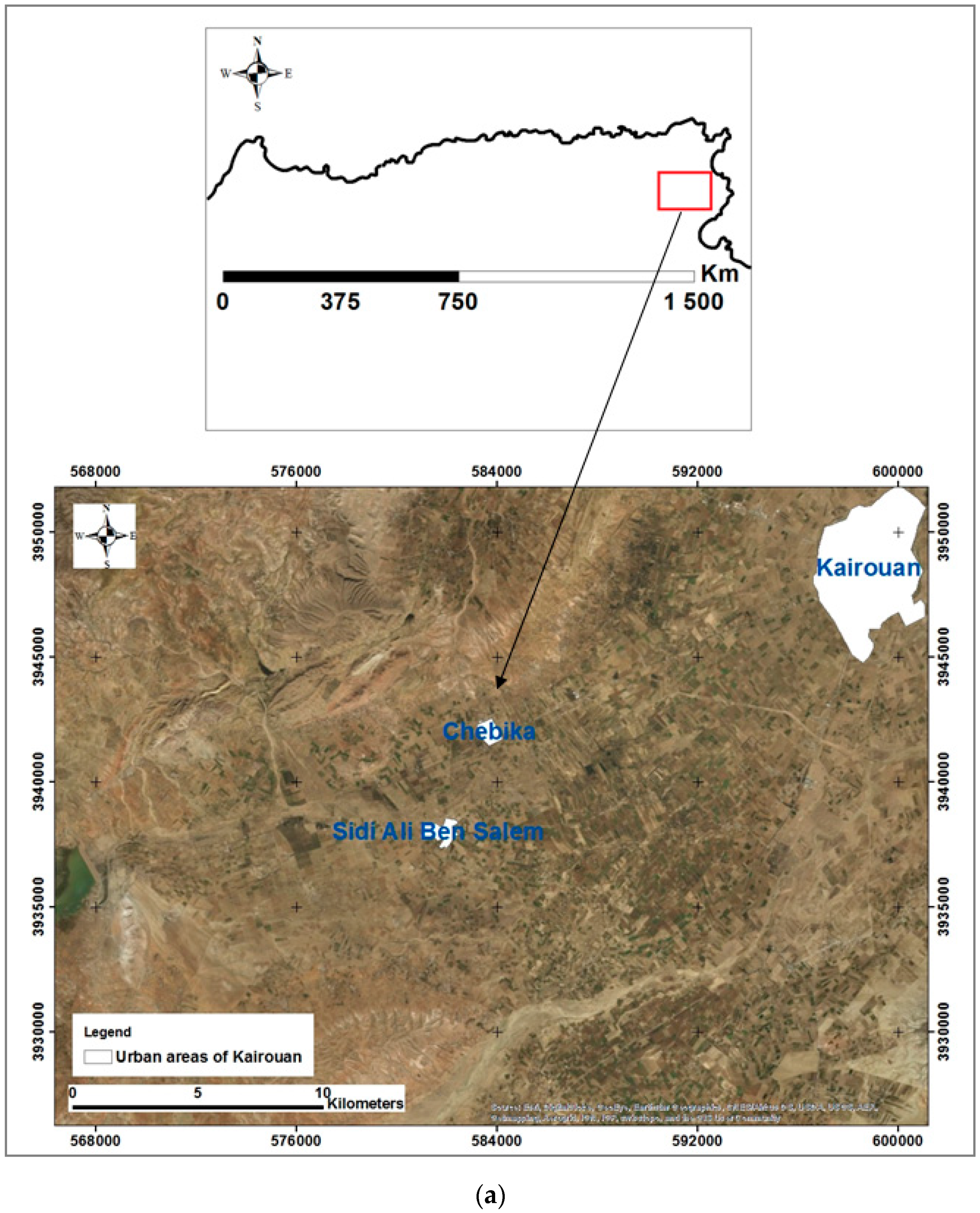
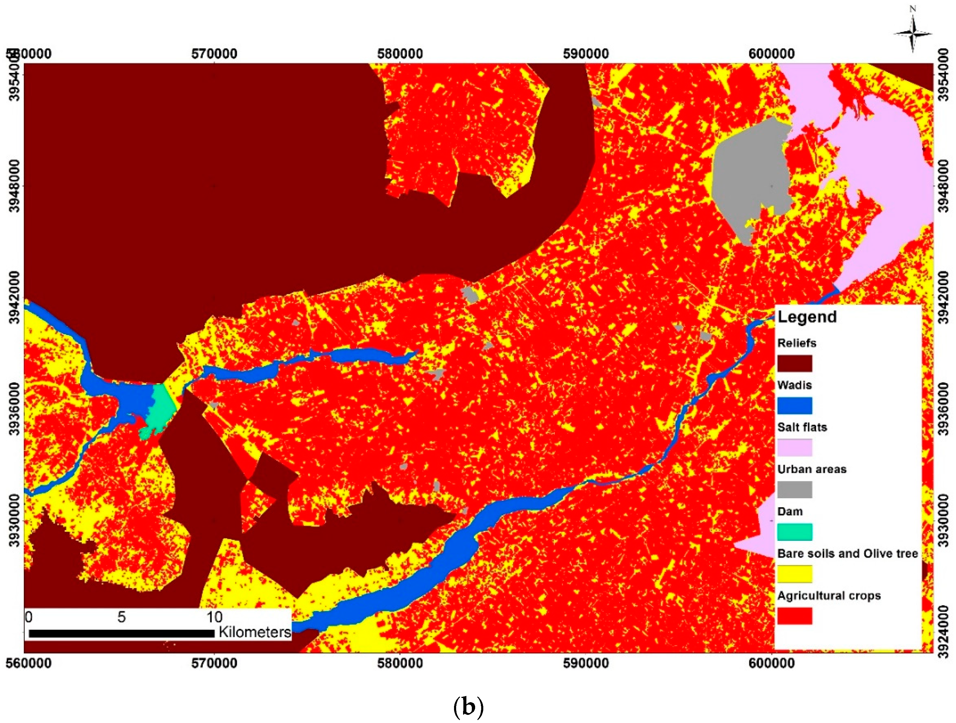
2.1. Study Site

The Kairouan plain (Central Tunisia: 9°53′57″E; 35°34′51″N; Figure 1a) is a semi-arid, typically agricultural region. Its flat topography is characterized by widespread cultivation (cereal crops and market gardening) together with arboriculture, which is dominated mainly by olive tree plantations [53]. The area has dry summer seasons, with an average temperature of approximately 30 °C during the hottest months (July and August), and wet winters. Precipitation is variable, with frequent periods of drought and an annual average rainfall of approximately 300 mm. The mean annual potential evapotranspiration is close to 1600 mm. The landscape in this area is dominated by agricultural plants (cereals and olive trees), as shown in Figure 1b, and the fields are covered by topsoil (5 cm in depth) consisting mainly of loam and clay.

Twenty reference fields with winter wheat crops (irrigated and rainfed wheat) were selected, and two campaigns were organized during the agricultural seasons (which start at the time of sowing and end after harvesting), from December 2015 to May 2016, and from December 2016 to March 2017. The first campaign was between December 2015 and May 2016; the second was between December 2016 and March 2017. These periods fall between the sowing and harvesting seasons of cereal crops [18]. The campaigns involved ground measurements and satellite acquisitions, and were carried out over the study site at regular intervals.

2.2. Ground Measurements

In situ soil moisture readings were recorded in selected reference fields (bare soil and wheat fields), and Sentinel-1 (S-1) radar observations were acquired, during the two cereal crop cycles (between December 2015 and March 2017). The in situ soil moisture and vegetation measurements were carried out on 38 different dates, at the same time as the radar acquisitions. For each reference field, twenty Thetaprobe measurements of volumetric soil moisture were made at a depth of 5 cm. These were calibrated using gravimetric measurements from previous campaigns [18]. Most of the fields were covered by smooth or moderately tilled soils.

The first agricultural season (2015–2016) was an extremely dry one, with a total annual rainfall of approximately 120 mm, recorded by the nearby INGC meteorological station (“Institut National des Grandes Cultures”; 9°56′16″E; 35°37′15″N). The soil moisture values were relatively low in the rainfed plots, and ranged between 3.9% (Vol.) and 18% (Vol.). In the case of the irrigated plots, the soil moisture values ranged between 5% (Vol.) and 39% (Vol.). The second agricultural season (2016–2017) was characterized by a relative higher average annual rainfall (approximately 240 mm), which was nevertheless lower than the long-term annual average, and soil moisture values ranging between 5% (Vol.) and 45% (Vol.).

An additional campaign was carried out between March and April 2017, in order to locate and collect information from several different agricultural fields (

Table 1. Scheduling of the study site measurement campaigns between 2015 and 2017.

Date Ranges	Campaigns	Fields Numbers
6 December 2015–28 April 2016	Theta Probe measurements	23
29 November 2016–30 March 2017	Theta Probe measurements	20
17 March 2017–17 April 2017	Irrigation investigation	74

), and to assess the differences in soil moisture characterizing rainfed and irrigated cereal crops. The data recorded during this campaign was later used to calibrate and validate the irrigation maps produced from the first two observation campaigns. Seventy-four plots were located over the Kairouan plain, corresponding to a total of 46 irrigated cereal crops and 28 rainfed wheat fields, with surface areas ranging between 2 and 25 ha.

The Kairouan plain has an extensive network of measuring stations, including meteorological and regular soil moisture stations. Four of the meteorological stations were installed in 2009, at Chebika (INGC), Skhira, Sidi Ali Ben Salem and Nasrallah. The closest station to the study site is that at Chebika, which provides meteorological data such as air temperature, relative humidity, global radiation, wind speed, atmospheric pressure and precipitation, at 30 min intervals.

2.3. Satellite Data

2.3.1. Sentinel-1

Sentienl-1A and Sentinel-1B images were acquired between December 2015 and March 2017. These satellites have the same orbital pattern, and are operated in the C-band (5.4 GHz), Interferometric Wideswath (IW) mode, with a spatial resolution of 10 m. Each satellite has a revisit period of 12 days, leading to a dual-satellite revisit period equal to six days. The sensors provide dual-polarization imagery (VV and VH) at an incidence angle ranging between 39° and 40°. This study used Level-1 ground range detection (GRD) products, derived from focused SAR images that were multi-looked and projected to a ground-range, using an Earth Ellipsoid Model.

The image processing was carried out using the Sentinel Application Platform (SNAP) toolbox. The first step in this process involved conversion of the signal, to obtain the backscattering coefficient. Terrain corrections were then applied, to correct for geometric distortions, using the Digital Elevation Model (DEM) proposed by the Shuttle Radar Topography Mission (SRTM), at a spatial resolution of 30 m. Finally, thermal noise removal and a Lee filter were applied, in order to reduce speckle effects in the images. The backscattering coefficient was averaged for each reference field. Seventy Sentinel-1 images recorded in the VV and VH polarizations, in both ascending and descending orbital modes, were successively downloaded and processed every six days.

2.3.2. Sentinel-2

Optical images of the study site were obtained from the Sentinel-2A satellite, on dates close to the Sentinel-1 images acquired between December 2015 and March 2017. The S-2A images were downloaded and processed from THEIA, a French open-source land data service center (https://www.theia-land.fr/).

The data was derived from cloud-free images with radiometric and atmospheric corrections. The Normalized Difference Vegetation Index (NDVI) was then computed, with Bands 4 and 8, which represent the Red (RED) and Near-Infrared (NIR) reflectances, using the expression:

$$NDVI=\left(NIR-RED\right)/\left(NIR+RED\right)$$

(1)

The values of NDVI were averaged for each reference field, and these ranged between 0.08 in the case of bare soils, and 0.8 in the case of dense vegetation.

Twenty-eight S-2 optical images were recorded on dates close to the S-1 radar acquisitions, with a delay of not more than ten days between the S-1 and S-2 images (in this area, cereal crops do not change significantly in a single week).

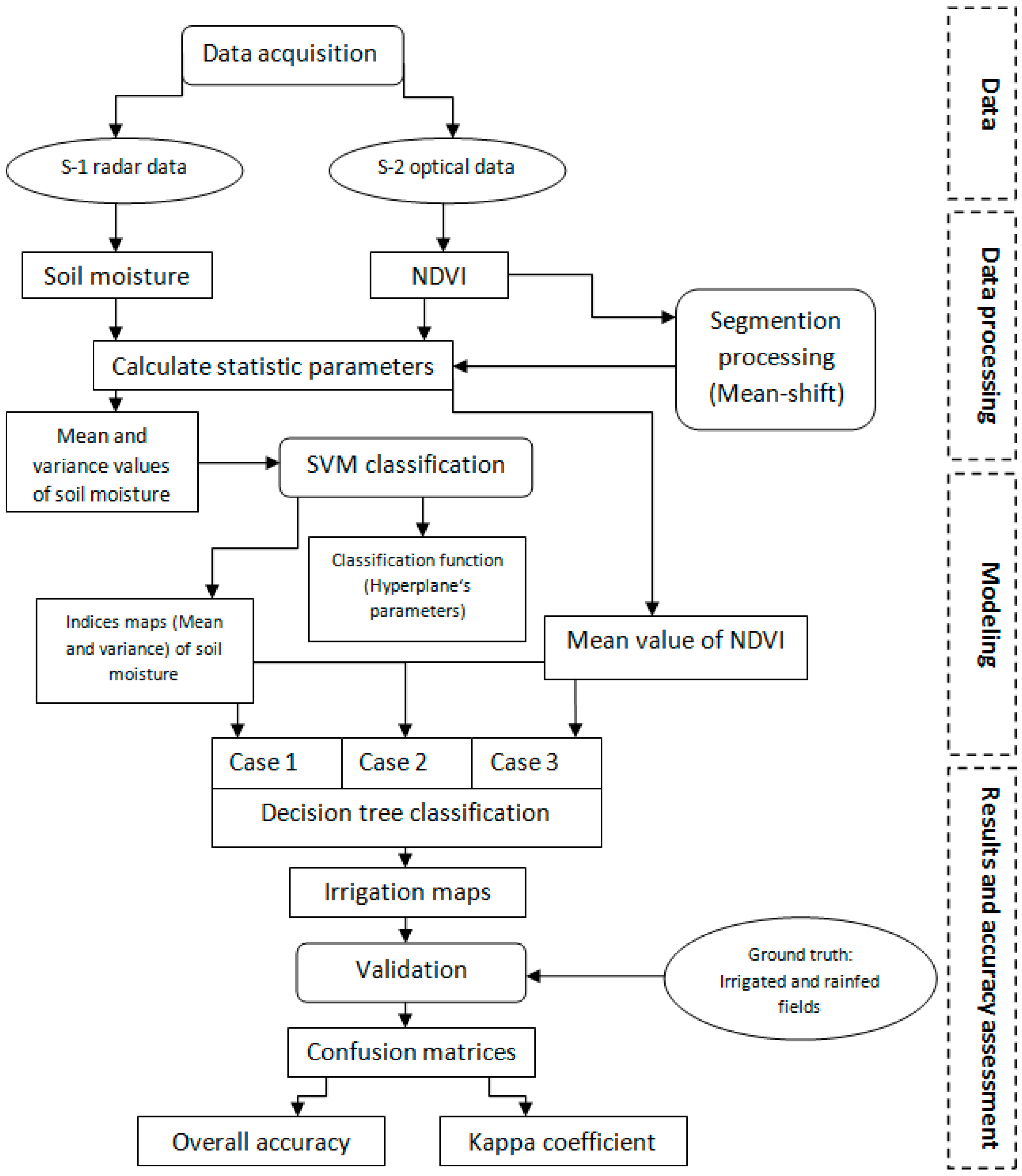
3. Methodology

3.1. Soil Moisture Retrieval Methodology

The soil moisture estimations were computed for bare soils and cereal fields. These need to be observed at a high spatial resolution, in order to facilitate the detection of irrigation events in individual fields. The proposed approach is based on the inversion of the WCM, coupled to an empirical soil backscattering model. The inversion algorithm comprises two successive phases, the first of which includes calibration of the model over the study site, and removal of all radar signal attenuation and/or scattering effects produced by the vegetation. The second step involves the implementation of an inversion algorithm to retrieve the soil moisture.

3.1.1. Water Cloud Model

The Water Cloud Model was developed by Attema and Ulaby [27], in order to simulate the characteristics of a radar signal when it is backscattered by the ground, and in any way affected by the soil surface moisture and plant canopies. The total backscattering coefficient (σ⁰) in this model is given by the following expressions:

$${\sigma }^0={\sigma }_{veg}^0+{\sigma }_{veg/soil}^0+{\tau }^2{\sigma }_{soil}^0$$

(2)

where

$${\tau }^2=\exp \left(-2 B V\sec \left(\theta \right)\right)$$

(3)

In Expression (2), the first term represents scattering due to the vegetation, and the second term, σ⁰_veg/soil, is related to multiple (“double-bounce”) scattering, which can often be neglected in the case of wheat scattering [54]. The third term represents soil scattering, attenuated by the vegetation cover.

The vegetation backscattering is modeled as:

$${\sigma }_{veg}^0=A V\cos \left(\theta \right)\left(1-{\tau }^2\right)$$

(4)

and the soil backscattering is modeled as:

$${\sigma }_{soil}^0=C {10}^{D.Mv}$$

(5)

The latter expression thus assumes that there is a linear relationship between the soil moisture and the radar signal expressed in dB, where C and D are calibration parameters, τ² is the two-way vegetation transmissivity, Mv is the soil moisture, θ is the incidence angle of the radar signal, and V is the vegetation parameter.

The calibration and validation of the WCM are described in a previous study [28]. The parameterization of the WCM was adapted to a wide range of soil moistures (between 5% (Vol.) and 45% (Vol.)), and NDVI values (between 0.14 and 0.8). The model is calibrated in two successive steps, the first of which uses bare soil reference fields to retrieve the parameters C and D, with the second step using vegetation-covered fields to retrieve the parameters A and B.

The fitted model allows the parameters A, B, C and D, (

Table 2. Water Cloud Model parameters for the VV polarization.

A	B	C	D	RMSE
0.06	0.42	−16.97	0.27	0.84 dB

), which depend on the type of canopy, to be determined. An earlier study [30] has also shown that the signal in the VV polarization is more sensitive to the soil surface parameter. For this reason, we consider the VV polarization only in the following section.

3.1.2. Inversion of the Water Cloud Model and Soil Moisture Retrieval

Following its calibration with the aforementioned parameters, the WCM is inverted and the soil moisture is computed. This inversion process makes use of the spatialized NDVI, derived from S-2 images and the backscattering coefficient. In the present study, we introduced a moving average filter with a 5 × 5 pixel window, in order to mitigate speckle artifacts on the resulting maps.

3.2. Irrigation Mapping Methodology

In this section, we propose a methodology for the identification of irrigated areas at the scale of individual fields, based on the interpretation of Sentinel-1 and Sentinel-2 images.

The structure of this algorithm is described by the flow chart in Figure 2. The key input data used in this process are the soil moisture maps produced by the inversion technique, and the values of NDVI derived from S-2 images.

The first step involves the processing of a segmented S-2 image, using NDVI data to generate meaningful image segments, including the agricultural fields of interest. The soil moisture and NDVI values are averaged for each of the segmented fields. The algorithm then makes use of the mean and variance of the soil moisture time series, and the mean value of the NDVI time series, in order to distinguish between irrigated and rainfed fields. Support Vector Machine and Decision Tree classification were incorporated into the process. Finally, the resulting irrigation maps are validated using selected reference fields.

3.2.1. Image Segmentation

To calculate the statistical parameters of the satellite products (mean and variance), the agricultural fields are assigned as homogenous segments, using an NDVI image derived from S-2 data. A segmentation algorithm (mean-shift) is then applied, and for each segment the mean NDVI, together with the mean and variance of the soil moisture, are computed.

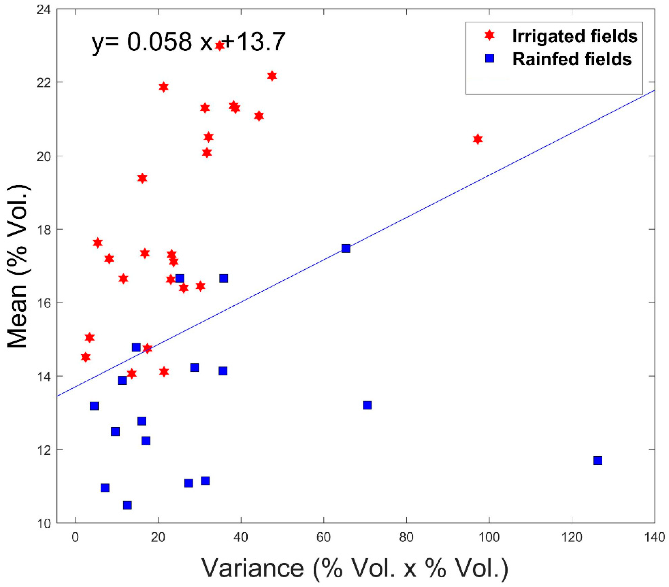
3.2.2. Support Vector Machine Classification

The purpose of the second step in the classification procedure is to distinguish between rainfed and irrigated areas. An initial classification step is implemented using a Support Vector Machine (SVM). The SVM is a supervised machine-learning algorithm, which has been widely applied to the classification of remote sensing images [55,56,57]. In the case of the present algorithm, classification is achieved by identifying a decision boundary that differentiates between the two classes. This boundary is generally an optimal hyperplane for linear, separable patterns (Figure 3), which can be expressed as:

$$Y=ax+b$$

(6)

where a and b are the hyperplane parameters, with a equal to 0.058 and b equal to 13.7.

The input variables in the SVM classification are the mean and variance of the soil moisture time series, computed from the descending node radar data, which has a revisit time of six days.

A total of 74 training cereal crops (irrigated and rainfed fields) were assessed across the study site, and then separated into two datasets: 46 fields were used to compute the parameters of the hyperplane equation, in the SVM modeling step. The results of this classification are shown in Figure 3, in which the irrigated and rainfed fields lie respectively above and below the linear hyperplane, and the highest mean values of soil moisture correspond to irrigated fields. It can also be seen that the variance and mean value of the soil moisture product time series are correlated. This trend can be explained in terms of the relative aridity of the study site, where frequent changes in the soil moisture of irrigated fields, from initially dry to relatively wet conditions, are associated with an increase in the variance of this parameter.

3.2.3. Decision Tree Classification

The Decision Tree classifier has long been employed for land cover mapping [58,59], to distinguish between various classes of agricultural area using indices derived from remote sensing data. The method developed in the present study applies the Decision Tree classification, using mean and variance maps of soil moisture together with a map of mean NDVI values, to separate the irrigated from the rainfed areas. This classification is based firstly on the use of maps of mean NDVI values only. It is then associated with the SVM classification, using the hyperplane parameters, together with the soil moisture parameters. Finally, the irrigation/rainfed classification is completed by combining the soil moisture parameters with the mean value of NDVI, leading to the production of irrigation maps. The 28 reference fields, which were not included in the 70 training fields, were used to validate the irrigated and rainfed fields identified by the classification algorithm.

4. Results

4.1. Validation and Mapping of Soil Moisture

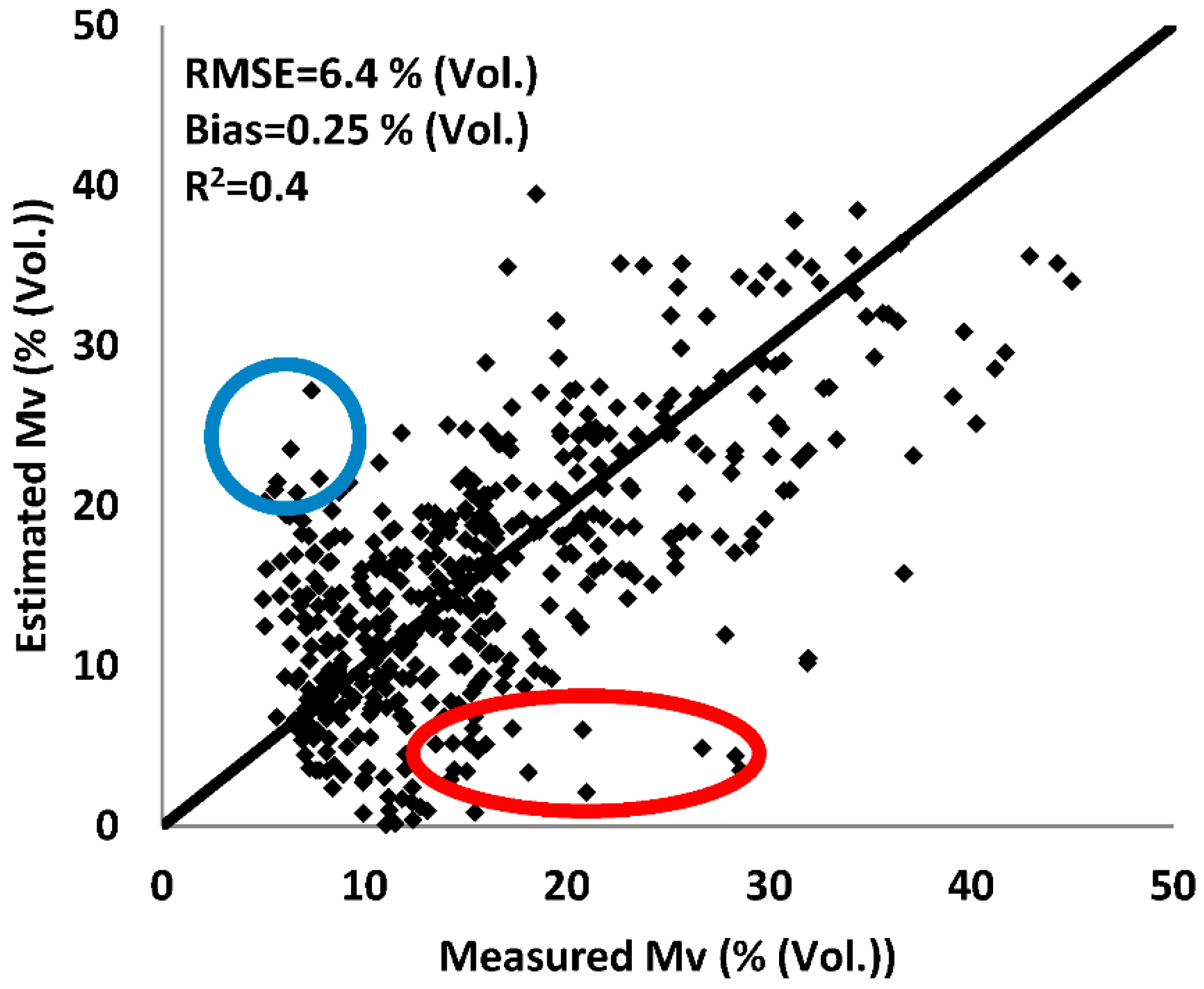
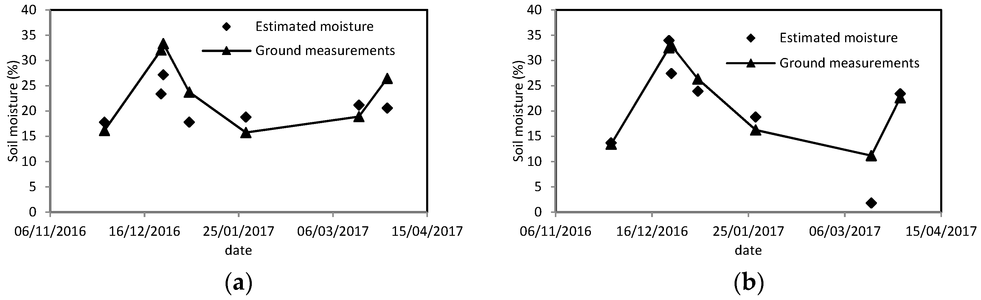
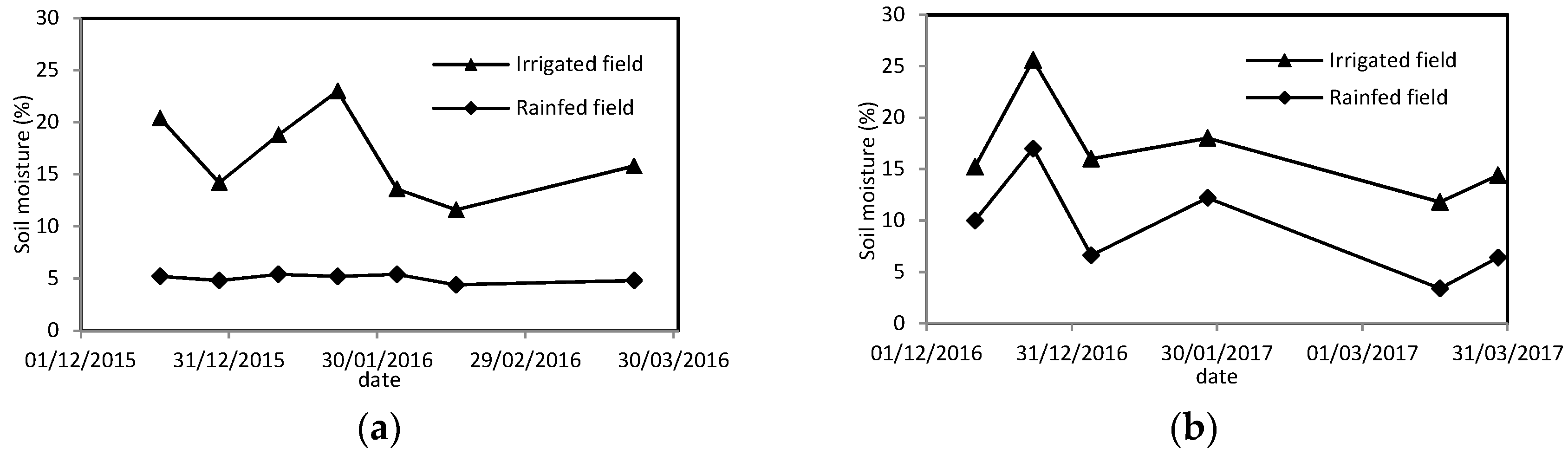
4.1.1. Validation of the Proposed Inversion Against Ground Measurements

The first validation is achieved by comparing the estimated water content with the ground measurements, acquired by the Theta Probe sensor on the reference fields, for soil moisture conditions ranging from dry to wet. Figure 4 shows the good agreement found between the measured and estimated soil moistures (derived from data in the VV polarization), for NDVI values ranging between 0.08 and 0.7. With these results, the RMSE is 6.4% (Vol.), the bias is 0.25% (Vol.), and the coefficient of determination R² is equal to 0.4 (with p-value < 0.01).

Figure 5 plots the estimated and measured (Theta probe) values of soil moisture as a function of time, for two different reference fields, showing that the remotely sensed estimations are in good agreement with the ground truth measurements.

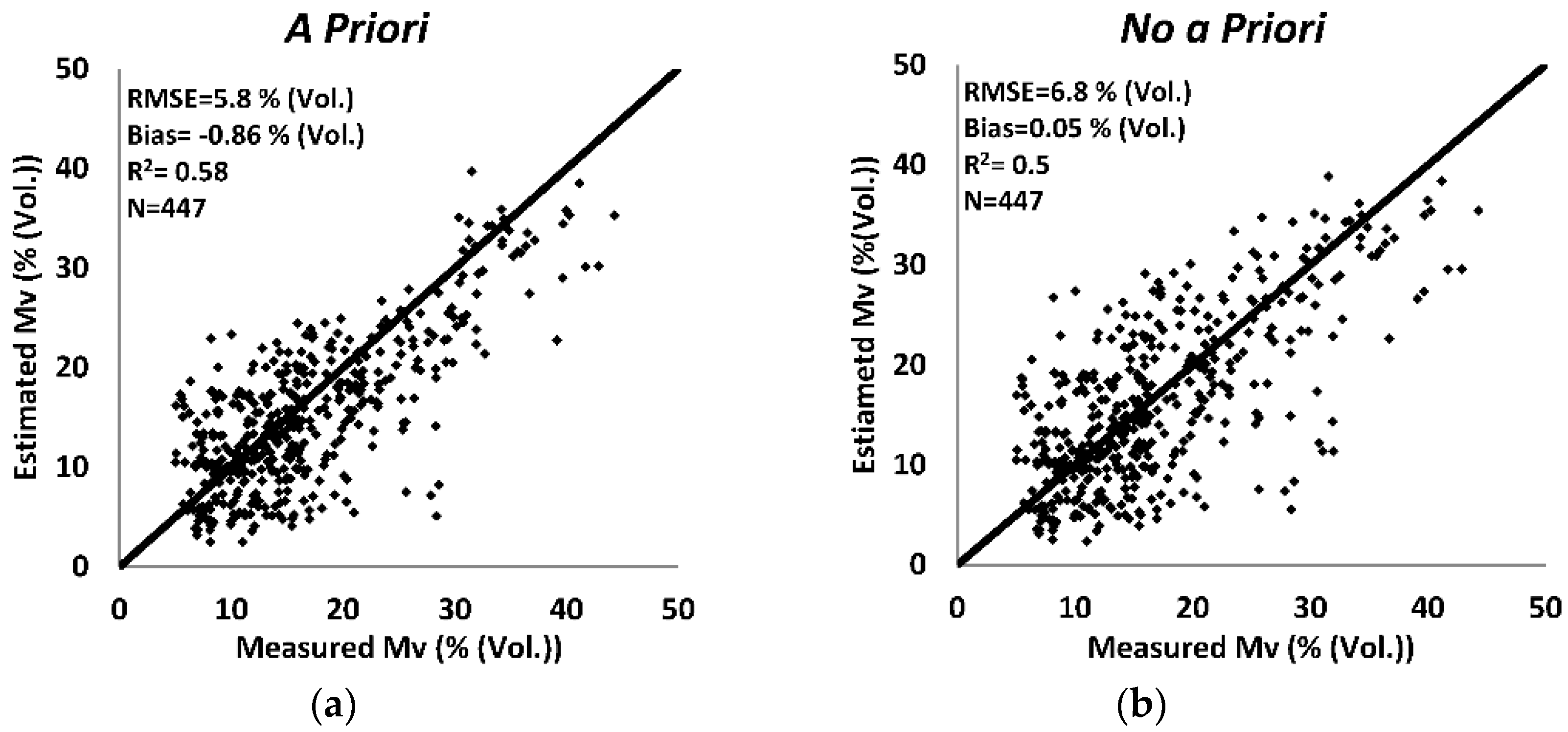
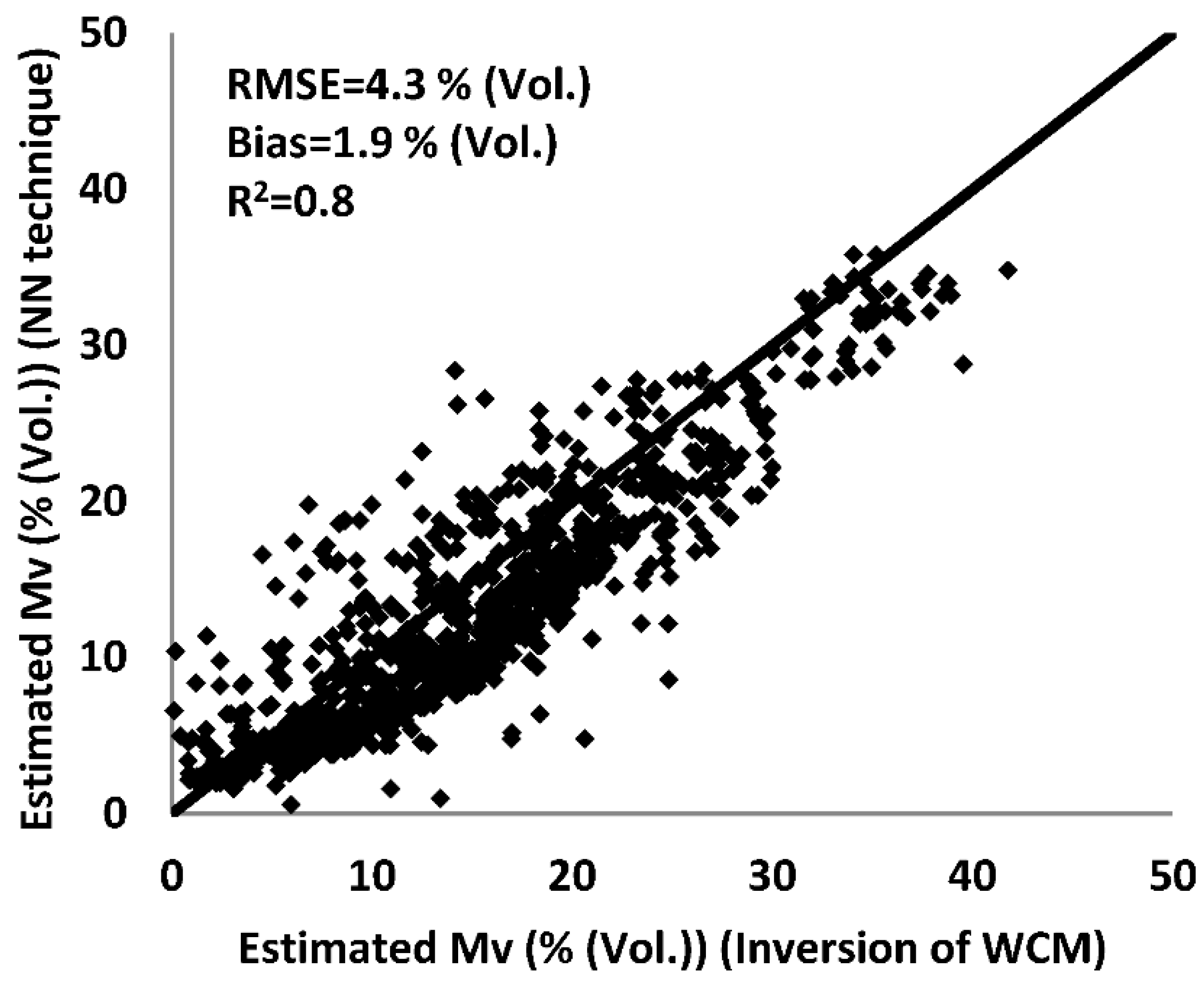
4.1.2. Validation of Soil Moisture Products Computed by Inversion, Using Neural Networks

(a) Neural Network products

A Neural Network (NN) technique for soil moisture mapping, based on the inversion of radar signals, has been proposed by El Hajj et al. [36]. This NN uses the WCM, coupled with the Integral Equation Model (IEM), and is trained using C-band SAR data in the VV and VH polarizations, together with NDVI data derived from optical S-2 images. Although, in an effort to improve the soil moisture estimations, the NN can include meteorological data to provide the network with a priori information concerning rainfall events, it can also be used without this information. In practice, rainfall has a significant influence on the soil and is strongly related to its surface moisture content. After a long period of drought, the soil becomes very dry, with low soil moisture values (Mv between 2% and 25% (Vol.)). Sudden bouts of heavy rain then lead to high levels of soil moisture (Mv between 25% and 40% (Vol.)).

In this context, NNs can be established for two distinct cases:

• no a priori information concerning the soil moisture
• availability of a priori information concerning the soil moisture: dry to wet or very wet soil.

This approach was shown to perform very well in the south of France [36], with an RMSE equal to 5.5% (Vol.) in the absence of a priori soil moisture information, and 4% (Vol.) in the presence of a priori information, for dry soils. In the case of wet soils, this technique led to an RMSE of 6.9% (Vol.) without a priori information, and 5.1% (Vol.) with a priori information.

Figure 6 shows the performance of the NN over the Merguellil site, for both cases (with and without a priori soil moisture information). In the absence of a priori information, the estimated values of Mv have an RMSE equal to 6.8% (Vol.) and a coefficient of determination (R²) equal to 0.5 (p-value < 0.01). When a priori information is available, the agreement between predicted and measured values of soil moisture is improved, and estimations with an RMSE equal to 5.8% (Vol.), and a coefficient of determination R² equal to 0.58 (p-value < 0.01).

(b) Comparing NN estimations with the proposed inversion products

Here, the soil moisture obtained with the NN and a priori information is compared with the values of soil moisture computed using direct inversion of the WCM (Figure 7), showing that these two products are highly correlated, with a coefficient of determination R² equal to 0.8, an RMSE of 4.3% (Vol.) and a bias of 1.9% (Vol.). Despite the limitations and simplicity of the inversion methodology, the results obtained with the NN validation show that it can accurately estimate the soil moisture.

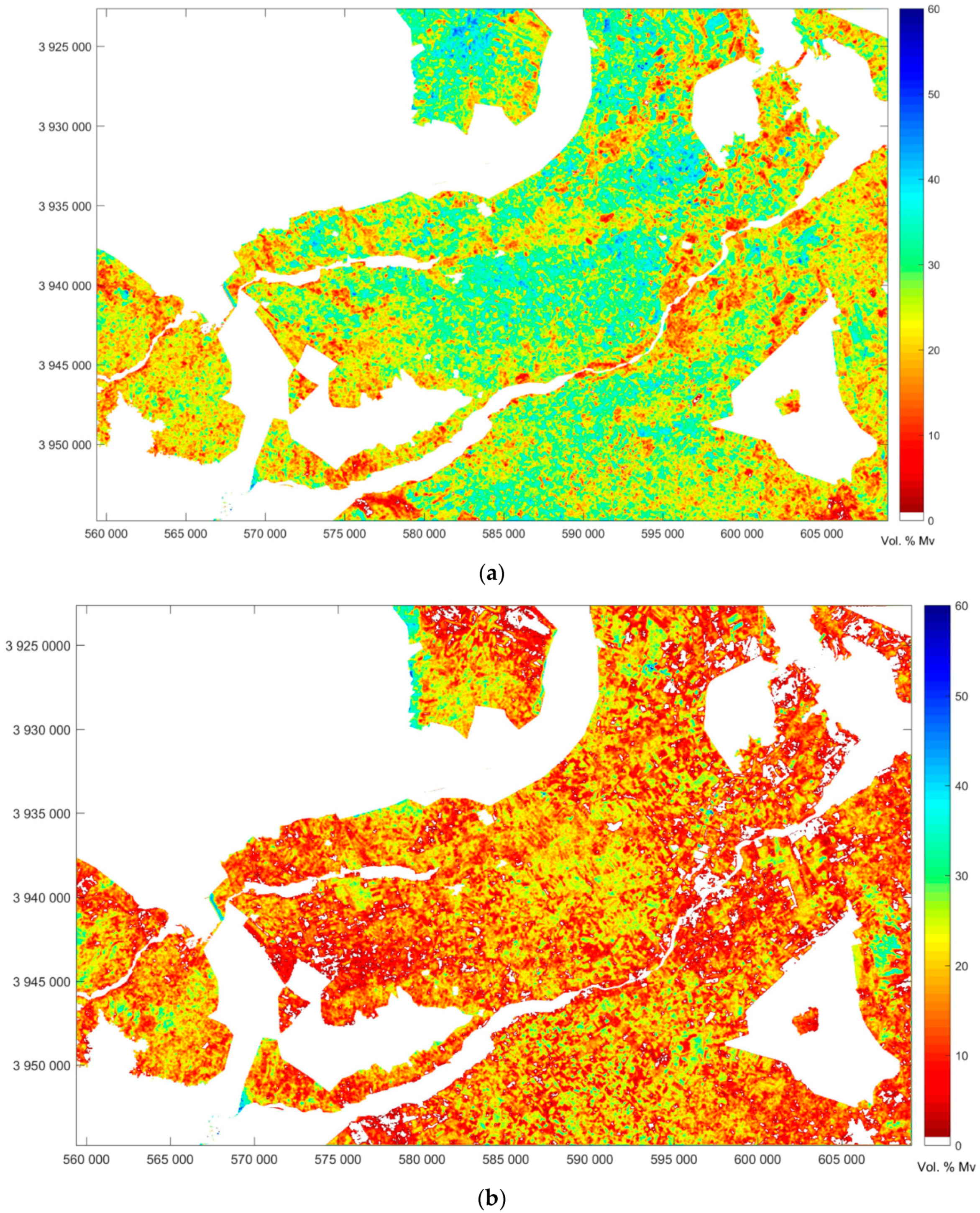
4.2. Soil Moisture Mapping

Figure 8 provides examples of the resulting soil moisture maps, computed for the study site by inverting the WCM. Two specific dates selected in order to analyze the soil moisture values obtained for the whole study site, for two specific cases: a wet period (24 December 2016), and a dry period (20 July 2016). The results obtained for these two cases are significantly different, as a consequence of their differences in terms of seasonal and meteorological conditions (rainfall).

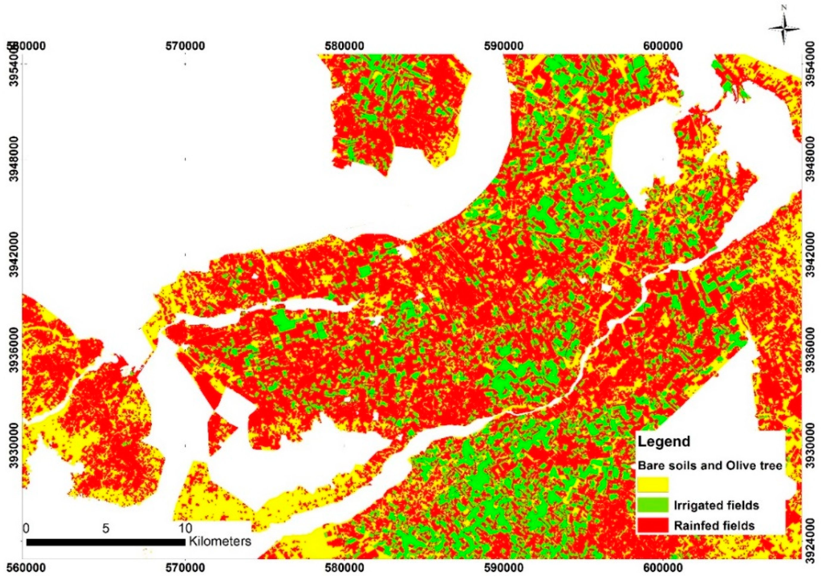
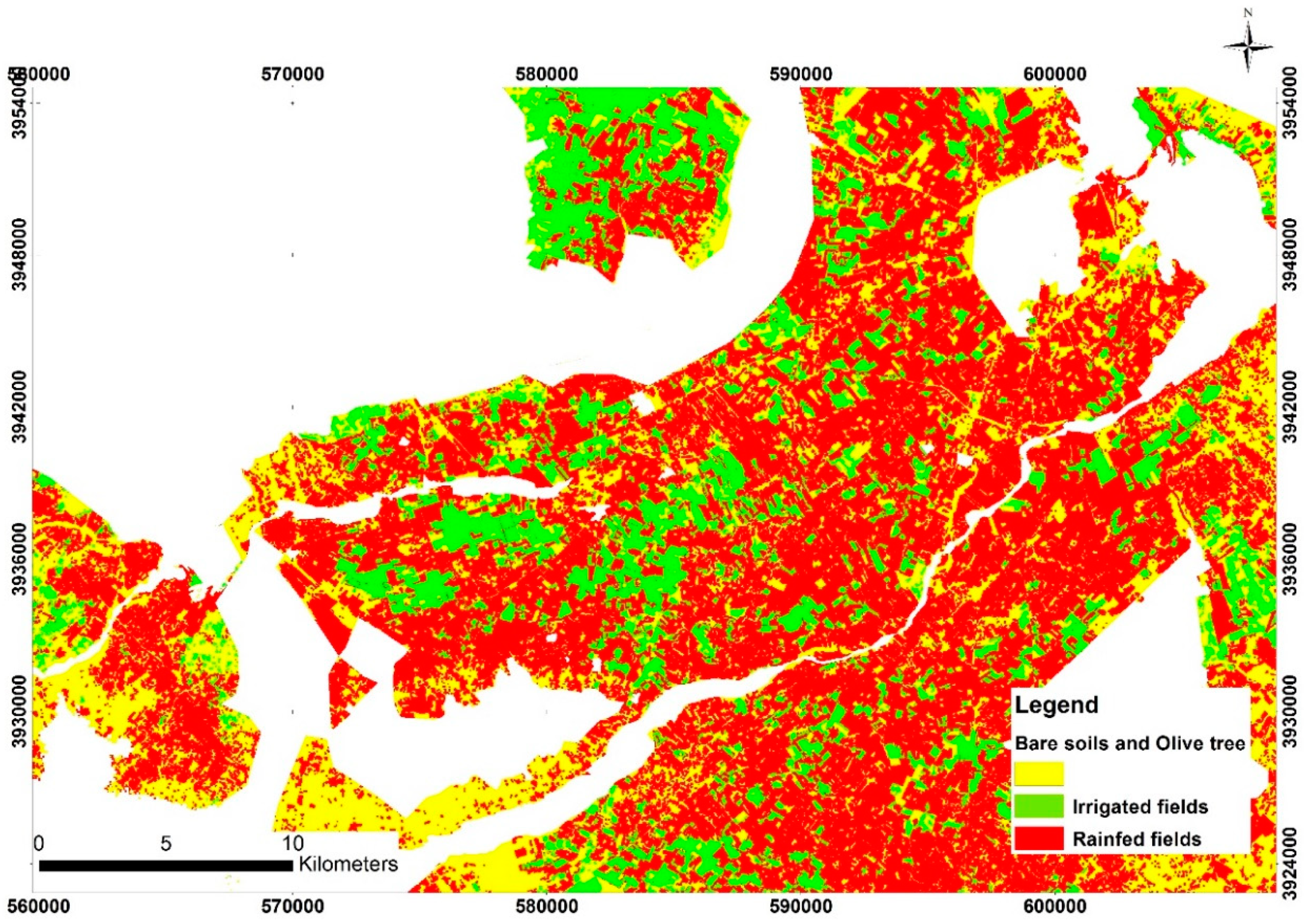
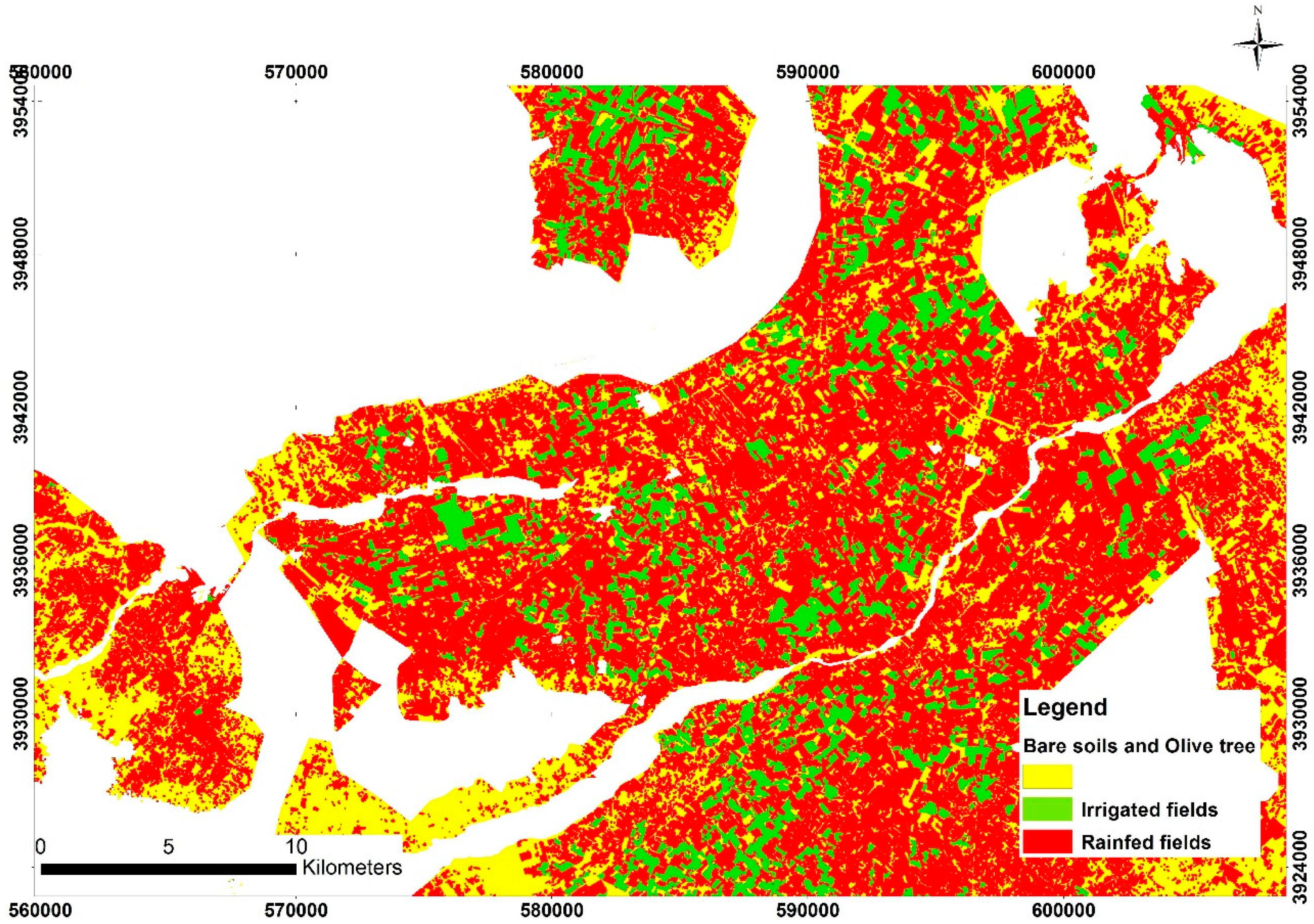
4.3. Irrigation Mapping

A mask is first applied to the images, in order to eliminate high ground, lakes or ponds, dams, urban areas, salt flats, and olive fields.

Three cases are then considered for the classification of irrigated and rainfed areas:

-

classification using mean NDVI values only

-

classification using soil moisture parameters (mean and variance) only

-

classification using the mean and variance of soil moisture, combined with the mean values of NDVI.

The irrigation results corresponding to the above three cases are shown in Figure 9, Figure 10, Figure 11 and Figure 12. These patterns of irrigation were then analyzed in greater detail, in order to identify the irrigated and non-irrigated fields on the study site. For this, confusion matrices were used to compare the pixels of each field with the resulting irrigation map. The resulting confusion matrices, used for the Decision Tree classification, are listed in

Table 3. Classification accuracy when the NDVI is assessed.

Classes		Reference
		Irrigated Pixels	Rainfed Pixels	Total
Classified	Irrigated pixels	1381	335	1716
	Rainfed pixels	616	334	950
	Total	1997	669	2666
Overall accuracy	58.1%
Kappa coefficient (K)	0.12

,

Table 4. Classification accuracy when the soil moisture is assessed.

Classes		Reference
		Irrigated Pixels	Rainfed Pixels	Total
Classified	Irrigated Pixels	1652	70	1722
	Rainfed Pixels	74	978	1052
	Total	1726	1048	2774
Overall Accuracy	77.2%
Kappa coefficient (K)	0.58

and

Table 5. Classification accuracy when both soil moisture and NDVI are assessed.

Classes		Reference
		Irrigated Pixels	Rainfed Pixels	Total
Classified	Irrigated pixels	1554	3	1557
	Rainfed pixels	270	1112	1382
	Total	1824	1115	2939
Overall accuracy	71.8%
Kappa coefficient (K)	0.52

. They summarize the accuracy statistics in terms of the Kappa coefficient, which is a standardized indicator of the overall accuracy of the validation step. This coefficient measures the strength of the agreement between the classification algorithm and the ground truth measurements, thus indicating the accuracy of each class, established with the validation data set. These classifications are based on a Decision Tree classifier.

● Classification based on NDVI statistical parameters

With this approach, the only classification parameter used to discriminate between fields was the mean value of NDVI, derived from the time series of NDVI images acquired during the month of March (Figure 9). This is the period during which cereals experience their most rapid growth. Earlier dates were not considered, because the sowing dates varied from one field to another. In the absence of any change in irrigation, this could significantly affect the measured values of NDVI. An empirical threshold of 0.6 was used to separate the irrigated from the non-irrigated fields. A field with a mean value of NDVI greater than 0.6 is thus interpreted as having irrigated crops, whereas fields with a lower NDVI are considered to be rainfed. This threshold can be shifted, in accordance with the climatic conditions and agricultural practices of the studied region.

The relatively poor accuracy (58.1%) of this “NDVI classification” is shown in Table 3.

● Classification using soil moisture statistics only

With this approach, we use soil moisture alone as a parameter to discriminate between irrigated and non-irrigated fields, without the NDVI index (Figure 11). Using the SVM algorithm, we compute the hyperplane parameters from the mean and variance of soil moisture values, which are estimated from the time series (January to end of March). The hyperplane is then used to separate the irrigated from the non-irrigated fields. In this region, the irrigation of cereal fields generally begins in early January, whereas the period of maximum vegetation growth occurs towards the end of March; soil moisture estimations are limited by a maximum NDVI of approximately 0.7 [36].

Figure 10 provides two examples of typical soil moisture product time series, for the 2015–2016 and 2016–2017 agricultural seasons, corresponding to irrigated and rainfed fields. During the studied seasons, soil moisture estimations were not computed for cases in which the weather (cloud cover) during the 15 preceding days had hindered the acquisition of suitable Sentinel-2 images. In both cases, we observed a significant difference between the moisture levels of irrigated and rainfed fields. This difference was particularly strong in the case of the driest season (2015–2016), during which very low values of soil moisture were observed in the rainfed fields.

The overall classification accuracy achieved with the soil moisture parameter is better than that obtained using the NDVI: 77.2%, with a Kappa coefficient (K) equal to 0.58 (Table 4).

● Classification using statistical parameters derived from both soil moisture and NDVI

With this approach, a decision tree classification is used based on three statistical parameters: the mean value of NDVI for the month of March, using the same threshold (0.6) as described above, and the mean and variance of the soil moisture (Figure 12). Thresholds were applied to the SVM algorithm, based on two statistical parameters: the mean and variance of the soil moisture time series. In the second approach, the values of soil moisture computed for the period between the beginning of January and the end of March are considered.

The combined use of these three indicators leads to good results, with an overall classification accuracy of 71.8% (Table 5).

5. Discussion

5.1. Soil Moisture Estimation

Soil moisture retrievals were computed using two different approaches, using optical and radar data at high spatial resolution. The first approach was based on the direct inversion of the WCM and the second one used the NN techniques. The two methods provided good results, with an RMSE approximately equal to 6% (Vol.), and are highly correlated. However, overestimations and underestimations of the approach, as shown in Figure 4 and Figure 6, are explained by dense vegetation cover and rough field.

The overestimation of soil moisture (in particular, the data points identified with a blue circle in Figure 4 is attributed to errors produced in the case of rough soil reference fields. In practice, as the proposed soil backscattering model simplifies the soil roughness to a uniform value for all fields, the soil moisture retrieved for fields with high roughness levels tends to be overestimated. For dense cereal crops with the highest values of NDVI (above 0.65, corresponding to the data points identified by a red ellipse in Figure 4), the proposed algorithm underestimates the soil moisture.

Two specific dates were selected to analyze the soil moisture maps. Figure 8a shows the soil moisture map, derived from the S-1 image acquired on 24 December 2016, revealing high levels of soil moisture across the site: most of the soil moisture values lie in the range between 25% (Vol.) and 45% (Vol.). The higher values correspond to a period characterized by a cumulative rainfall of 85 mm during the five days preceding the estimations, recorded by the meteorological station (INGC) within the site. Figure 8b (20 July 2016) corresponds to a dry date: the lowest values of soil moisture range between 5% (Vol.) and 20% (Vol.). In the case of this observation, no precipitation had been recorded during the months of June and July. The significantly higher values of soil moisture revealed in certain areas are interpreted as the consequence of local irrigation in selected fields.

5.2. Irrigation Mapping

The first generated irrigation map was based on the mean value of NDVI (Figure 9, Table 3). This classification provided the lowest results with an overall accuracy of 58.1%. Relatively frequent confusions occur between rainfed and irrigated fields, due to two different factors: (a) in the case of the 2016–2017 season, which was not particularly dry, even non-irrigated fields could attain high values of NDVI; (b) as fertilizers are not used by all farmers, higher NDVI levels could be observed for non-irrigated, but fertilized fields, rather than for irrigated fields without fertilization. These constraints, combined with the absence of optical images on certain dates (due to cloud cover), illustrate the limitations of an approach-based solely on the interpretation of NDVI.

Figure 11 provided the resulting irrigation map from the classification using only soil moisture parameters (Mean and variance value). As shown in Table 3, the classification provided the highest accuracy. This improvement can be attributed to the fact that a relatively high level of soil moisture is a more reliable indicator of irrigation than a relatively high level of NDVI. The soil moisture indicator is particularly important in the semi-arid environment of the proposed site, where the number of rainfall events is generally very small, and the level of evaporation is high, leading to a substantial difference in the behavior of soil moisture, between irrigated and non-irrigated fields.

The third classification used the soil moisture parameters and the mean value of NDVI. The inclusion of soil moisture clearly improves the accuracy of the classification. However, the case using soil moisture parameters only yields, slightly better results, thus showing that the inclusion of the NDVI slightly degrades the classification accuracy. These results are typical for a semi-arid site with a small number of rainfall events, a high level of evaporation, and variable practices in terms of the use of fertilizers.

6. Conclusions

In semi-arid areas, water resources are becoming increasingly scarce. For this reason, it is important to propose scenarios for the improved management of these natural resources, in an effort to ensure the future protection and development of the agricultural sector.

The aim of the present study is to generate operational irrigation maps on an annual basis, distinguishing between irrigated and rainfed areas, for the management of irrigation and the implementation of agricultural strategies, at a high spatial resolution.

In an initial step, operational approaches were proposed for the retrieval of soil moisture maps, at the scale of individual fields on the semi-arid Kairouan plain in central Tunisia.

With the arrival of the Sentinel-1 and Sentinel-2 constellations, it has now become feasible to produce soil moisture products at high spatial resolutions and relatively high temporal frequencies.

The approach proposed in this study is based on the inversion of the WCM, using radar data recorded in the VV polarization and NDVI data derived from optical images. The estimated values of soil moisture are validated using ground measurements and a Neural Network (NN) moisture product. Consistent results are obtained when the two satellite moisture products are compared, with an RMSE of 4.3% (Vol.) and a bias of 1.9% (Vol.) between the two estimations.

A classification algorithm is proposed for the mapping of irrigated and rainfed areas over the Kairouan plain. The first approach to this classification uses a Support Vector Machine (SVM) to distinguish between irrigated and rainfed areas, based on soil moisture parameters (mean and variance). A Decision Tree classification is then used to produce irrigation maps with several simulations based on these parameters, for three specific cases: a classification based on mean NDVI values for agricultural fields; a classification based on the mean and variance of soil moisture time series; and lastly a classification based on the mean and variance of soil moisture time series, together with the mean values of NDVI. The highest overall classification accuracy (77%) is achieved when the soil moisture parameters only are used. The lowest accuracy is achieved when the mean values of NDVI only are used. In the present study, the added NDVI information to the soil moisture data decreased the quality of the classification. This outcome is probably due to the limited ability of NDVI to distinguish between irrigated and non-irrigated fields, in the specific context of our semi-arid study site, which is characterized by high levels of evaporation, rare and infrequent rainfall events, and the limited application of fertilizers. Despite the considerable potential of Sentinel-1 and Sentinel-2 data for the production of irrigation maps, in certain cases their 6-day revisit period could be insufficient for the observation of all irrigation and rainfall events. In a forthcoming study, these methods will be tested in more humid regions, in an effort to examine the changes in empirical thresholds considered in this study, as well as the limitations and specific characteristics of the optical NDVI and soil moisture products when applied to the analysis of irrigation practices.

References

- Alexandratos, N.; Bruinsma, J. World Agriculture towards 2030/2050: The 2012 Revision; ESA Working Paper No. 12–13; Food and Agriculture Organization of the United Nations: Rome, Italy, 2012. [Google Scholar]
- Doungmanee, P. The nexus of agricultural water use and economic development level. Kasetsart J. Soc. Sci. 2016, 37, 38–45. [Google Scholar] [CrossRef]
- Simonneaux, V.; Lepage, M.; Helson, D.; Metral, J.; Thomas, S.; Duchemin, B.; Cherkaoui, M.; Kharrou, H.; Berjami, B.; Chebhouni, A. Estimation spatialisée de l’ évapotranspiration des cultures irriguées par télédétection: Application à la gestion de l’irrigation dans la plaine du haouz (Marrakech, Morocco). Sécheresse 2009, 20, 123–130. [Google Scholar]
- Saadi, S.; Simonneaux, V.; Boulet, G.; Raimbault, B.; Mougenot, B.; Fanise, P.; Ayari, H.; Lili-Chabaane, Z. Monitoring irrigation Consumption using high resolution NDVI image time series: Calibration and validation in the Kairouan plain (Tunisia). Remote Sens. 2015, 7, 13005–13028. [Google Scholar] [CrossRef]
- Adeyemi, O.; Grove, I.; Peets, S.; Norton, T. Advanced Monitoring and Management Systems for Improving Sustainability in Precision Irrigation. Sustainability 2017, 9, 353. [Google Scholar] [CrossRef]
- Kharrou, M.; Page, M.L.; Chehbouni, A.; Simonneaux, V.; Er-Raki, S.; Jarlan, L.; Ouzine, L.; Khabba, S.; Chehbouni, G. Assessment of Equity and Adequacy of Water Delivery in Irrigation Systems Using Remote Sensing-Based Indicators in Semi-Arid Region, Morocco. Water Resour. Manag. 2013, 27, 4697–4714. [Google Scholar] [CrossRef]
- Ambika, A.K.; Wardlow, B.; Mishra, V. Data Descriptor: Remotely sensed high resolution irrigated area mapping in India for 2000 to 2015. Sci. Data 2016, 3, 160118. [Google Scholar] [CrossRef] [PubMed]
- Ozdogan, M.; Gutman, G. A new methodology to map irrigated areas using multi-temporal MODIS and ancillary data: An application example in the continental US. Int. J. Remote Sens. 2008, 112, 3520–3537. [Google Scholar] [CrossRef]
- Satalino, G.; Mattia, F.; Ruggieri, S.; Rinaldi, M. LAI estimation of agricultural crops from optical data at different spatial resolution. In Proceedings of the 2009 IEEE International Geoscience and Remote Sensing Symposium (IGARSS 2009), Cape Town, South Africa, 12–17 July 2009. [Google Scholar] [CrossRef]
- Eklundh, L.; Jin, H.; Schubert, P.; Guzinski, R.; Heliasz, M. An Optical Sensor Network for Vegetation Phenology Monitoring and Satellite Data Calibration. Sensors 2011, 11, 7678–7709. [Google Scholar] [CrossRef]
- Kuusk, A. Monitoring of vegetation parameters on large areas by the inversion of a canopy reflectance model. Int. J. Remote Sens. 1998, 19, 2893–2905. [Google Scholar] [CrossRef]
- Leprieur, C.; Verstraete, M.M.; Pinty, B. Evaluation of the performance of various vegetation indices to retrieve vegetation cover from AVHRR data. Remote Sens. Rev. 1994, 10, 265–284. [Google Scholar] [CrossRef]
- Gutman, G.; Ignatov, A. The derivation of the green vegetation fraction from NOAA/AVHRR data for use in numerical weather prediction models. Int. J. Remote Sens. 1998, 19, 1533–1543. [Google Scholar] [CrossRef]
- Ghahremanloo, M.; Mobasheri, M.R.; Amani, M. Soil moisture estimation using land surface temperature and soil temperature at 5 cm depth. Int. J. Remote Sens. 2018. [Google Scholar] [CrossRef]
- Yang, Y.; Guan, H.; Lon, D.; Liu, B.; Qin, G.; Qin, J.; Batelaan, O. Estimation of Surface Soil Moisture from Thermal Infrared Remote Sensing Using an Improved Trapezoid Method. Remote Sens. 2015, 7, 8250–8270. [Google Scholar] [CrossRef]
- Zribi, M.; Gorrab, A.; Baghdadi, N. A new soil roughness parameter for the modeling of radar backscattering over bare soil. Remote Sens. Environ. 2014, 152, 62–73. [Google Scholar] [CrossRef]
- Saux-Picart, S.; Ottlé, C.; Decharme, B.; André, C.; Zribi, M.; Perrier, A.; Coudert, B.; Boulain, N.; Cappelaere, B. Water and Energy budgets simulation over the Niger super site spatially constrained with remote sensing data. J. Hydrol. 2009, 375, 287–295. [Google Scholar] [CrossRef]
- Zribi, M.; Chahbi, A.; Lili Chabaane, Z.; Duchemin, B.; Baghdadi, N.; Amri, R.; Chehbouni, A. Soil surface moisture estimation over a semi-arid region using ENVISAT ASAR radar data for soil evaporation evaluation. Hydrol. Earth Syst. Sci. 2011, 15, 345–358. [Google Scholar] [CrossRef]
- Zribi, M.; Pardé, M.; Boutin, J.; Fanise, P.; Hauser, D.; Dechambre, M.; Kerr, Y.; Leduc-Leballeur, M.; Reverdin, G.; Skou, N.; et al. CAROLS: A New Airborne L-Band Radiometer for Ocean Surface and Land Observations. Sensors 2011, 11, 719–742. [Google Scholar] [CrossRef]
- King, C.; Lecomte, V.; Le Bissonnais, Y.; Baghdadi, N.; Souchère, V.; Cerdan, O. Remote-sensing data as an alternative input for the ‘STREAM’runoff model. Catena 2005, 62, 125–135. [Google Scholar] [CrossRef]
- Oh, Y.; Sarabandi, K.; Ulaby, F.T. An empirical model and an inversion technique for radar scattering from bare soil surfaces. IEEE Trans. Geosci. Remote Sens. 1992, 30, 370–382. [Google Scholar] [CrossRef]
- Dubois, P.C.; Van Zyl, J.; Engman, T. Measuring soil moisture with imaging radars. IEEE Trans. Geosci. Remote Sens. 1995, 33, 915–926. [Google Scholar] [CrossRef]
- Baghdadi, N.; Choker, M.; Zribi, M.; El-hajj, M.; Paloscia, S.; Verhoest, N.; Lievens, H.; Baup, F.; Mattia, F. A new empirical model for radar scattering from bare soil surfaces. Remote Sens. 2016, 8, 920. [Google Scholar] [CrossRef]
- Fung, A.K.; Li, Z.; Chen, K.S. Backscattering from a randomly rough dielectric surface. IEEE Trans. Geosci. Remote Sens. 1992, 30, 356–369. [Google Scholar] [CrossRef]
- Baghdadi, N.; King, C.; Chanzy, A.; Wigneron, J.P. An empirical calibration of the integral equation model based on SAR data, soil moisture and surface roughness measurement over bare soils. Int. J. Remote Sens. 2002, 23, 4325–4340. [Google Scholar] [CrossRef]
- Baghdadi, N.; Holah, N.; Zribi, M. Calibration of the integral equation model for SAR data in C-band and HH and VV polarizations. Int. J. Remote Sens. 2006, 27, 805–816. [Google Scholar] [CrossRef]
- Attema, E.P.W.; Ulaby, F.T. Vegetation modeled as a water cloud. Radio Sci. 1978, 13, 357–364. [Google Scholar] [CrossRef]
- Prévot, L.; Champion, I.; Guyot, G. Estimating surface soil moisture and leaf area index of a wheat canopy using a dual-frequency (C and X bands) scatterometer. Int. J. Remote Sens. 1993, 46, 331–339. [Google Scholar] [CrossRef]
- Kumar, K.; Hari Prasad, K.S.; Arora, M.K. Estimation of water cloud model vegetation parameters using a genetic algorithm. Hydrol. Sci. J. 2012, 57, 776–789. [Google Scholar] [CrossRef]
- Bousbih, S.; Zribi, M.; Lili-Chabaane, Z.; Baghdadi, N.; El Hajj, M.; Gao, Q.; Mougenot, B. Potential of Sentinel-1 Radar Data for the Assessment of Soil and Cereal Cover Parameters. Sensors 2017, 17, 2617. [Google Scholar] [CrossRef] [PubMed]
- Baghdadi, N.; El Hajj, M.; Zribi, M.; Bousbih, S. Calibration of the Water Cloud Model at C-Band for Winter Crop Fields and Grasslands. Remote Sens. 2017, 9, 969. [Google Scholar] [CrossRef]
- El Hajj, M.; Baghdadi, N.; Zribi, M.; Belaud, G.; Cheviron, B.; Courault, D.; Charron, F. Soil moisture retrieval over irrigated grassland using X-band SAR data. Remote Sens. Environ. 2016, 176, 202–218. [Google Scholar] [CrossRef]
- Elshorbagy, A.; Parasuraman, K. On the relevance of using artificial neural networks for estimating soil moisture content. J. Hydrol. 2008, 362, 1–18. [Google Scholar] [CrossRef]
- Paloscia, S.; Pampaloni, P.; Pettinato, S.; Santi, E. Generation of soil moisture maps from ENVISAT/ASAR images in mountainous areas: A case study. Int. J. Remote Sens. 2010, 31, 2265–2276. [Google Scholar] [CrossRef]
- Paloscia, S.; Pettinato, S.; Santi, E.; Notarnicola, C.; Pasolli, L.; Reppucci, A. Soil moisture mapping using Sentinel-1 images: Algorithm and preliminary validation. Int. J. Remote Sens. 2013, 134, 234–248. [Google Scholar] [CrossRef]
- El Hajj, M.; Baghdadi, N.; Zribi, M.; Bazzi, H. Synergic use of Sentinel-1 and Sentinel-2 images for operational soil moisture mapping at high spatial resolution over agricultural areas. Remote Sens. 2017, 9, 1292. [Google Scholar] [CrossRef]
- Hassan-Esfahani, L.; Torres-Rua, A.; Jensen, A.; McKee, M. Assessment of Surface Soil Moisture Using High-Resolution Multi- Spectral Imagery and Artificial Neural Networks. Remote Sens. 2015, 7, 2627–2646. [Google Scholar] [CrossRef]
- Mishra, V.; Cruise, J.F.; Hain, C.R.; Mecikalsk, J.R.; Anderson, M.C. Development of soil moisture profiles through coupled microwave–thermal infrared observations in the southeastern United States. Hydrol. Earth Syst. Sci. 2018, 22, 4935–4957. [Google Scholar] [CrossRef]
- Jackson, T.J.; Cosh, M.H.; Bindlish, R.; Starks, P.J.; Bosch, D.D.; Seyfried, M.; Goodrich, D.C.; Moran, M.S.; Du, J. Validation of Advanced Microwave Scanning Radiometer Soil Moisture Products. IEEE Trans. Geosci. Remote Sens. 2010, 48, 4256–4272. [Google Scholar] [CrossRef]
- Le Morvan, A.; Zribi, M.; Baghdadi, N.; Chanzy, A. Soil moisture profile effect on radar signal measurement. Sensors 2008, 8, 256–270. [Google Scholar] [CrossRef]
- Zribi, M.; Kotti, F.; Wagner, W.; Amri, R.; Shabou, M.; Lili-Chabaane, Z.; Baghdadi, N. Soil moisture mapping in a semi-arid region, based on ASAR/Wide Swath satellite data. Water Resour. Res. 2014, 50, 823–835. [Google Scholar] [CrossRef]
- Gao, Q.; Zribi, M.; Baghdadi, N.; Escorihuela, M.J. Synergetic Use of Sentinel-1 and Sentinel-2 Data for Soil Moisture Mapping at 100 m Resolution. Sensors 2017, 17, 1966. [Google Scholar] [CrossRef]
- Tomer, S.K.; Al Bitar, A.; Sekhar, M.; Zribi, M.; Bandyopadhyay, S.; Sreelash, K.; Sharma, A.K.; Corgne, S.; Kerr, Y. Retrieval and Multi-scale Validation of Soil Moisture from Multi-temporal SAR Data in a Tropical Region. Remote Sens. 2015, 7, 8128–8153. [Google Scholar] [CrossRef]
- Thiruvengadachari, S. Satellite sensing of irrigation pattern in semiarid areas: An Indian study. Photogramm. Eng. Remote Sens. 1981, 47, 1493–1499. [Google Scholar]
- Gao, Q.; Zribi, M.; Escorihuela, M.; Baghdadi, N.; Segui, P. Irrigation Mapping Using Sentinel-1 Time Series at Field Scale. Remote Sens. 2018, 10, 1495. [Google Scholar] [CrossRef]
- Thenkabail, P.S.; Schull, M.; Turral, H. Ganges and Indus river basin land use/land cover (LULC) and irrigated area mapping using continuous streams of MODIS data. Remote Sens. Environ. 2004, 95, 317–341. [Google Scholar] [CrossRef]
- Fieuzal, R.; Duchemin, B.; Jarlan, L.; Zribi, M.; Baup, F.; Merlin, O.; Dedieu, G.; Garatuza-Payan, J.; Watt, C.; Chehbouni, A. Combined use of optical and radar satellite data for the monitoring of irrigation and soil moisture of wheat crops. Hydrol. Earth Syst. Sci. 2011, 15, 1117–1129. [Google Scholar] [CrossRef]
- Dheeravath, V.; Thenkabail, P.S.; Chandrakantha, G.; Noojipady, P.; Reddy, G.P.O.; Biradar, C.M.; Gumma, M.K.; Velpuri, M. Irrigated areas of India derived using MODIS 500 m time series for the years 2001–2003. ISPRS J. Photogramm. Remote Sens. 2009, 65, 42–59. [Google Scholar] [CrossRef]
- Kamthonkiat, D.; Honda, K.; Turral, H.; Tripathi, N.K.; Wuwongse, V. Discrimination of irrigated and rainfed rice in a tropical agricultural system using SPOT VEGETATION NDVI and rainfall data. Int. J. Remote Sens. 2005, 26, 2527–2547. [Google Scholar] [CrossRef]
- Gumma, M.K.; Thenkabail, P.S.; Hideto, F.; Nelson, A.; Dheeravath, V.; Busia, D.; Rala, A. Mapping Irrigated Areas of Ghana Using Fusion of 30 m and 250 m Resolution Remote-Sensing Data. Remote Sens. 2011, 3, 816–835. [Google Scholar] [CrossRef]
- Jin, N.; Tao, B.; Ren, W.; Feng, M.; Sun, R.; He, L.; Zhuang, W.; Yu, Q. Mapping Irrigated and Rainfed wheat areas using multi-temporal satellite Data. Remote Sens. 2016, 8, 207. [Google Scholar] [CrossRef]
- Meier, J.; Zabel, F.; Mauser, W. A global approach to estimate irrigated areas—A comparison between different data and statistics. Hydrol. Earth Syst. Sci. 2018, 22, 1119–1133. [Google Scholar] [CrossRef]
- Gorrab, A.; Zribi, M.; Baghdadi, N.; Mougenot, B.; Fanise, P.; Lili Chabaane, Z. Retrieval of Both Soil Moisture and Texture Using TerraSAR-X Images. Remote Sens. 2015, 7, 10098–10116. [Google Scholar] [CrossRef]
- Ulaby, F.T.; Moore, R.K.; Fung, A.K. Microwave Remote Sensing Active and Passive; Artech House Publishers: Reading, MA, USA, 1986. [Google Scholar]
- Mountrakis, G.; Im, J.; Ogole, C. Support vector machines in remote sensing. A review. ISPRS J. Photogram. Remote Sens. 2011, 66, 247–259. [Google Scholar] [CrossRef]
- Pal, M.; Mather, P.M. Support vector machines for classification in remote sensing. Int. J. Remote Sens. 2005, 26, 1007–1011. [Google Scholar] [CrossRef]
- Huang, C.; Davis, L.; Townshend, J. An assessment of support vector machines for land cover classification. Int. J. Remote Sens. 2002, 23, 725–749. [Google Scholar] [CrossRef]
- Mclver, D.K.; Friedl, M.A. Using prior probabilities in decision-tree classification of remotely sensed data. Remote Sens. Environ. 2002, 81, 253–261. [Google Scholar] [CrossRef]
- Punia, M.; Joshi, P.K.; Prwal, M.C. Decision trees classification of land use cover for Delhi, India using IRS-P6 AWiFS data. Expert Syst. Appl. 2010, 38, 5577–5583. [Google Scholar] [CrossRef]