1. Introduction
The upcoming space missions Tandem-L and BIOMASS, plan to create a 3-D map of the global forest structure by means of synthetic aperture radar (SAR) tomography (TomoSAR), and monitor the global carbon cycle in a systematic manner. Particularly, BIOMASS will signify the first space-borne P-band SAR [
1].
TomoSAR is a powerful remote sensing (RS) technique that allows the 3-D imaging of volumetric targets, recovering the vertical distribution of the backscattered power for each range-azimuth resolution cell [
2,
3]. For the case of forested scenes, as the one considered in this work, the retrieval of the forest height and the above-ground biomass, constitute the key components for the study of the global carbon cycle [
1,
4]. The TomoSAR RS technique aids at the recovery of such parameters due to its distinctive ability to monitor the 3-D inner structure of volumetric targets, gathering information about the nature and location of the ongoing scattering processes.
Forested scenes are characterized by a continuous distribution of scatterers along the vertical axis, and are not only composed of few prominent point-type scatterers. For such scenarios, SAR sensors operating in longer wavelengths, e.g., L- and P-band, are commonly chosen, having better sensitivity to the contributions from both the ground surface and the vegetation layers [
5,
6]. Specifically, the high penetration capability of the transmitted wave at P-band, allows for observing the ground surface even in a dense forest.
The TomoSAR nonlinear inverse problem at hand is commonly treated applying modern spatial spectral analysis (SSA) techniques, within the direction-of-arrival (DOA) estimation framework [
3]. The conventional non-parametric matched spatial filter (MSF) and Capon beamforming techniques [
3,
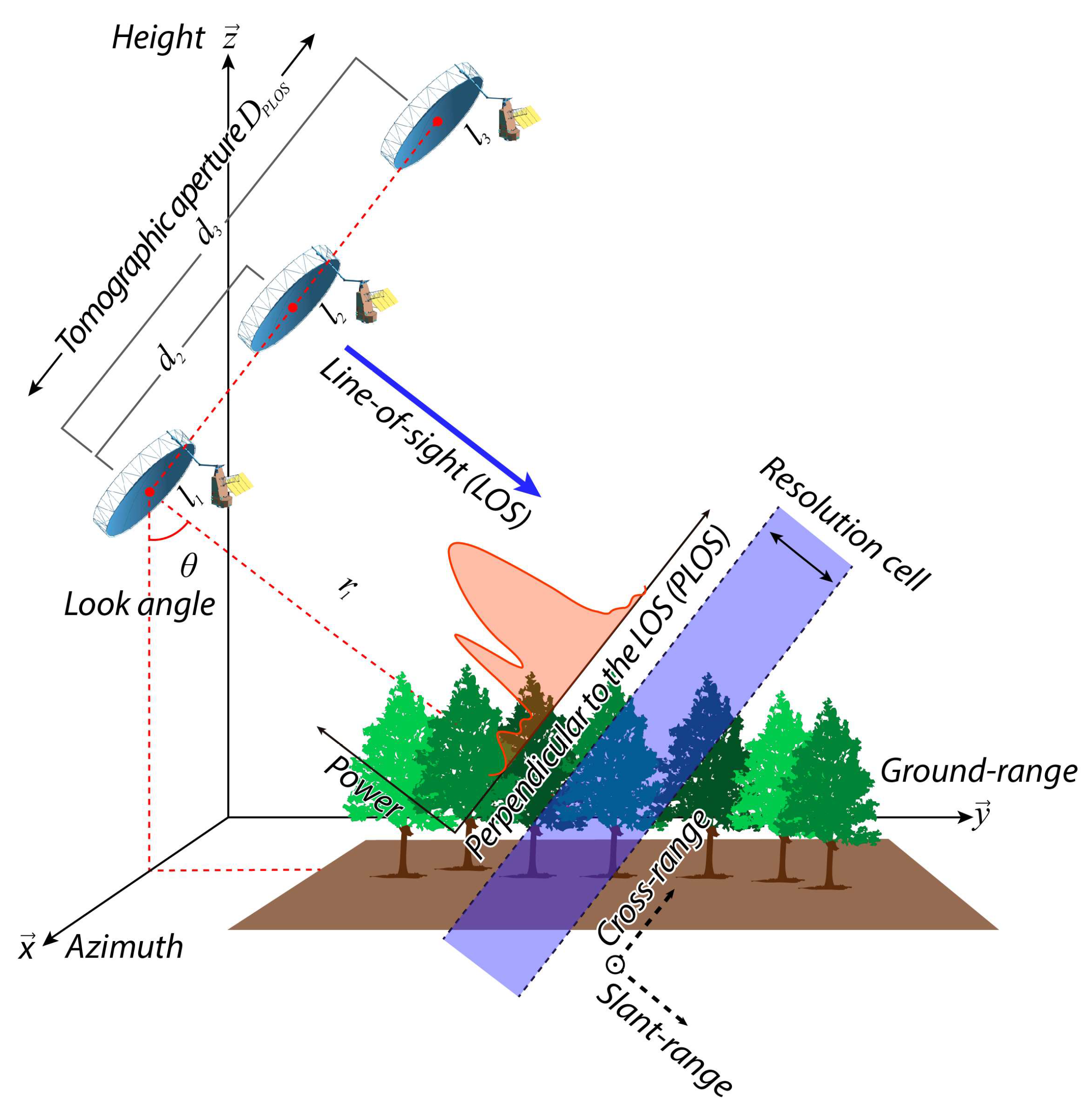
7] are well suited to cope with scenarios characterized by the presence of distributed scatterers, since these techniques recover an estimate of the continuous power spectrum pattern (PSP). Particularly, Capon provides enhanced resolution when the number of processed looks/snapshots is sufficiently high to avoid the rank deficiency of the data covariance matrix. Nonetheless, the resolution capability of such SSA-based estimators highly depends on the total baseline span, the so-called tomographic aperture (refer to
Figure 1). Furthermore, irregular sampling and non-uniform acquisition constellations introduce artifacts and increase the ambiguity levels, sacrificing the overall achievable image quality.
Taking advantage of the sparse representations of the perpendicular to the line-of-sight (PLOS) profiles in the wavelet domain, super-resolved compressed sensing (CS)-based approaches [
8,
9] are also employed to deal with the TomoSAR inverse problem. However, CS-based techniques often imply a considerable computational burden, due to their iterative nature and due to the non-availability of adapted efficient convex optimization algorithms.
Overcoming the above-mentioned disadvantages of the conventional MSF and Capon beamforming methods, in the real-world TomoSAR operating scenarios, and with significantly lower computational burden in comparison to the wavelet-based CS techniques, a new nonparametric multi-stage approach for feature enhanced TomoSAR imaging is addressed in this paper. The proposed new approach combines the descriptive experiment design regularization (DEDR) framework [
10,
11], for enhanced image reconstruction, with the sparsity preserving image refinement in the wavelet transform (WT) domain [
12,
13]. First, high resolution imagery is recovered from the MSF initial estimates via the virtual adaptive beamforming (VAB)-based processing with convergence guaranteed projections onto convex sets (POCS) (Section 15.4.5 in Reference [
14]). Further refinement with suppression of artifacts is performed via the sparsity preserving wavelet domain thresholding (WDT).
The new addressed multi-stage iterative method, called WAVAB (WDT-refined VAB), operates robustly in scenarios with non-regular constellation geometries and only a few available snapshots. Additionally, the aggregation of the sum of Kronecker products (SKP) decomposition technique [
15,
16] at the pre-processing stage improves ground and canopy separation and allows for the application of different better suited TomoSAR imaging techniques, on the ground and canopy structural components, separately.
The feature enhancing capabilities of the WAVAB TomoSAR imaging technique are corroborated via processing E-SAR airborne real data of the German Aerospace Center, providing detailed volume height profiles reconstruction as an alternative to the existing most prominent competing non-parametric SSA-based approaches.
2. Problem Phenomenology
Consider a TomoSAR acquisition constellation composed by
L tracks as a linear array. In a discrete-form representation, the TomoSAR data signal vector
y represents the set of
L focused signals for a specified azimuth-range position, and is related to the complex random scene reflectivity vector
s via the linear equation of observation (EO) [
3,
7],
in which the
steering matrix
is composed of
M L-dimensional steering vectors
that contain the interferometric phase information, associated to a source located at the PLOS elevation position
above the reference focusing plane, which, for a certain elevation position
is given by [
7],
where
is the two-way vertical wavenumber between the master track and the
l-th acquisition positions. Here,
stands for the carrier wavelength,
is the incidence angle,
is the slant-range distance between the master track and the considered target, and
is the PLOS-oriented baseline distance between the master position and the
l-th acquisition position, as depicted in
Figure 1.
Vectors
s,
n and
y in the EO (1), define the vectors composed of the decomposition coefficients
,
and
, of the finite-dimensional approximations of the continuous signal
S, noise
N and observation
Y fields, respectively; and matrix
is the signal formation operator (SFO) that maps
S →
Y, the source Hilbert signal space
S onto the observation Hilbert signal space
Y [
10].
In the current study, we avoid any parameterization or structurization of the scattering field model. Thus, we resort to a model in which the scatterers are assumed to be distributed over unknown support regions over the pixel-framed sensing search area. In the case of absense of scatterers in certain zones (e.g., scenes composed of a mixture of point-like and distributed scatterers), the relevant scattering field is sparse, and the sparsity supports are unknown to the observer. For such a case, vectors
s,
n and
y represent complex random Gaussian zero-mean vectors, which are characterized by their corresponding correlation matrices [
7,
10]
and
where
stands for the Hermitian conjugate operator,
is the power spectral density of the white noise power [
3] and
is the expectation operator.
Vector
b at the principal diagonal of the diagonal matrix
, composed of the averaged entries
at each
m-th PLOS elevation position,
defines the backscattering power, referred to also as the PSP, i.e., the second order statistics of the complex reflectivity vector
s.
The inverse TomoSAR imaging problem at hand resides on reconstructing an optimal estimate of the vertical profile of the illuminated scene backscattered power reflectivity map, for each observed range-azimuth resolution cell, given the complex (multi-look) SAR data recordings y. Recall that in this contribution, we intend to follow the DEDR-WDT optimization strategy and develop the new nonparametric TomoSAR WAVAB optimal solver.
3. Related State-of-the-Art Work
In order to retrieve a statistically optimal solution to the previously specified TomoSAR nonlinear inverse problem, the Bayes minimum risk (BMR) strategy [
17] is extended to the maximum-likelihood (ML) optimization approach, imposing no constraint on linearity and assuming no a priori knowledge about the probability density function (pdf) of the desired PSP vector
b.
Due to the intrinsic statistical nature of the physical phenomena, the TomoSAR data vector
y, in the EO (1), is customary modelled as a stochastic vector, which, in theory, represents an infinite number of different realizations of the data formation process. The pdf of such a complex-valued zero-mean Gaussian vector
y is given by [
18]
We define then, the log-likelihood function of vector
b as the logarithm of the conditional pdf
[
19],
in which the terms that do not contain
b are ignored and the scene characteristics are retrieved from the measurement statistics presented by the data covariance matrix
[
3,
7],
where
indicates one of
J independent realizations (looks) of the SAR signal acquisitions.
The ML solution is then reduced to the minimization problem
with the objective function
. As it has been proven in Reference [
19], minimization of (11) with respect to the PSP vector
b, related to
, is equivalent to minimizing the covariance fitting Stein’s loss and yields the ML-inspired estimator (Equation (32) in Reference [
19])
Taking into account the properties of the convergent Capon SSA estimates of the PSP (power reflectivity), which in a coordinate/pixel form are given by [
3,
7]
making use of the fixed-point iterative implementation of the ML algorithm (12), as suggested in Reference [
19], and performing some algebraic manipulations, we find that the ML estimator (12) in the vector form,
, is algorithmically equivalent to the solver to the following equation (the transformation of (12) into the solver in (14) is detailed in Reference [
11])
with the real-valued measurement data statistics
the solution-depended weighted MSF data vector
and the solution-dependent weighted MSF imaging system point spread function (PSF) operator
where symbol
denotes the Schur-Hadamard (element-wise) matrix product. In (14) and (15), operator {⋅}
diag returns the vector at the principal diagonal of the embraced matrix; in (16),
represents the matrix-form ambiguity function (AF) operator of the MSF system that performs formation of the complex image
.
The initial estimate of the PSP
is formed as a square detected MSF output (here,
defines the element-wise square detection operator). To increase accuracy in the presence of signal-dependent (multiplicative) noise when retrieving
, multi-looking is performed through the averaging of adjacent values in the data covariance matrix
(10) or from multiple reduced resolution focalizations of the cell of interest via azimuth sub-apertures [
20].
4. Proposed TomoSAR-Adapted WAVAB Approach
Following the general DEDR methodology [
10,
11], first, we define the variational analysis (VA)-inspired metrics structure in the solution space, specified by the inner product
with the metric inducing matrix-form operator
where
I is the identity matrix,
defines the numerically approximated discrete-form Laplacian, computed applying the first-order finite difference operator
[
21] over the original
M-pixel formatted PLOS sensing direction
z. The weight parameters
,
,∈[0,1], scaled to the [0,1] interval, control the balance between the corresponding metrics measures in the image space
. In the general case,
,
, the Laplacian term in
tends to contrast the image high spatial frequency information; thus, contrast preservation regularization is implicitly considered [
22].
Next, to construct the WAVAB solver for the feature enhanced image reconstruction, in the positive cone solution set from , with the VA-inspired metric, we suggest to aggregate the image recovery transforms and the convergence guaranteed POCS into the multi-stage DEDR-structured solution rule (that we refer to as the WAVAB-optimal solver) . Application of such to solve (14) yields the desired feature enhanced TomoSAR image. The purpose of the proposed multi-stage solver is threefold:
(i) First, the action of operator transforms (14) into the implicit contractive mapping iterative scheme in the image space , with the VA-structured metric specified above.
(ii) Second, operator
defines a sparsity preserving POCS operator that clips off all entries lower than the user specified nonnegative sparsity promoting tolerance threshold
in the image/solution space. For the simplest (zero) assignment,
= 0,
defines the constraining projector onto the nonnegative convex cone solution set. Hence, incorporation of
,
, into the implicit iterative solver (19) guarantees its convergence, that is, a direct sequence from the fundamental theorem of POCS (Section 15.4.5 in Reference [
14]). These two cascade transforms,
, specify the iterative DEDR solver
where the adaptively weighted image vector
and the solution-dependent matrix-form PSF operator
, defined by (16), are updated at each
i-th iteration, and the metrics balancing factors
,
, are the user-specified degrees of freedom to compete between the overall enhanced image smoothing and contrast preservation regularization.
The iterative process is terminated at
, for which the user specified
-norm convergence control tolerance level
εTL is attained at some
i =
I (or the maximum admissible number of iterations is reached) [
11,
21]. In the experiments reported next, we followed the suggestions from Reference [
11] for the equi-balanced adjustment,
, which does not affect the overall convergence of (19) that is a direct sequence from the fundamental theorem of POCS.
(iii) Last, the composite transform operator
performs the discrete WT-based sparsity promoting (i.e., soft thresholding in the WT domain) transform of the last (
I-th) iteration of (19) into
where
defines the WDT-based sparsity promoting recovery operator, in which
denotes the (inverse) discrete WT,
represents the image recovered at the
t-th iteration of (20), and
is the element-wise Donoho’s soft thresholding (denoising) operator with a shrinkage parameter
, in which
denotes the function max(
f, 0) and
is the element-wise signum function [
12,
13]. In the experiments reported next, we adopted the Daubechies Symlet WT basis with four vanishing moments and three levels of decomposition, as suggested in the related works [
8,
9], and the median estimator for
[
13] that yields
= 0.0481 (for the 0…1 scale of
in
). The iterations in (20) are initialized by the previously reconstructed image (19), i.e.,
, and are terminated after attaining the asymptotic convergence, (in a conventional
discrepancy metric).
Incorporation of the POCS pre-conditioner into (20) guarantees its convergence and preservation of image non-negativity, i.e., consistency. The recovery performed at the last (T-th) iteration at the WDT processing stage (20) yields the desired WAVAB-optimally enhanced TomoSAR image .
The motivation for performing the second iterative process (20) is based on the orthogonal WT expansion of the PSP power image (at any iteration in (20))
, where
denotes the (inverse) DWT and
represents a vector of the wavelet coefficients defined as
. Due to the presumed orthogonality of the employed discrete WT, we have
=
, the identity operator [
23].
The feature enhanced TomoSAR images recovered at the DEDR-VAB stage (19) manifest sparse representations in the WT space with a few large coefficients and many very small ones. Thus, incorporation of the WDT-based iterative recovery stage in (20) provides additional image enhancement with suppression of the artifacts that may be produced by (19), performed via the sparsity promoting denoising in the WT domain with assured non-negativity and consistency preservation.
With the extensions treated, the multi-level DEDR-WDT regularization via multi-stage iterative processing (19), (20), guarantees well-conditioned solutions (in the Hadamard sense) to the TomoSAR nonlinear inverse problem in (14).
Notice that the ML-inspired solver in (12) becomes the Capon method [
3,
7] when
. Being (14) algorithmically equivalent to (12), the introduced WAVAB approach in (19) and (20) can be seen as a variant (refinement) of the Capon technique, adapted to the case when there are discrepancies between the measured data covariance matrix
and the actual (modelled) data correlation matrix
. Moreover, by constructions, the computations in (19) do not involve any matrix inversion at all iteration steps, which differs our approach from Capon beamforming, that requires inversions of
; the ML-based method in (12), that requires inversions of
; and from the previous DEDR-related developments in [
10,
11], that require inversions of
, meaning, that the latter techniques are inapplicable for feature enhanced reconstruction of sparse tomographic PSP scenes, in which some of the elements of vector
equal to zero.
In summary, the introduced WAVAB approach is implemented as follows:
6. Numerical Examples
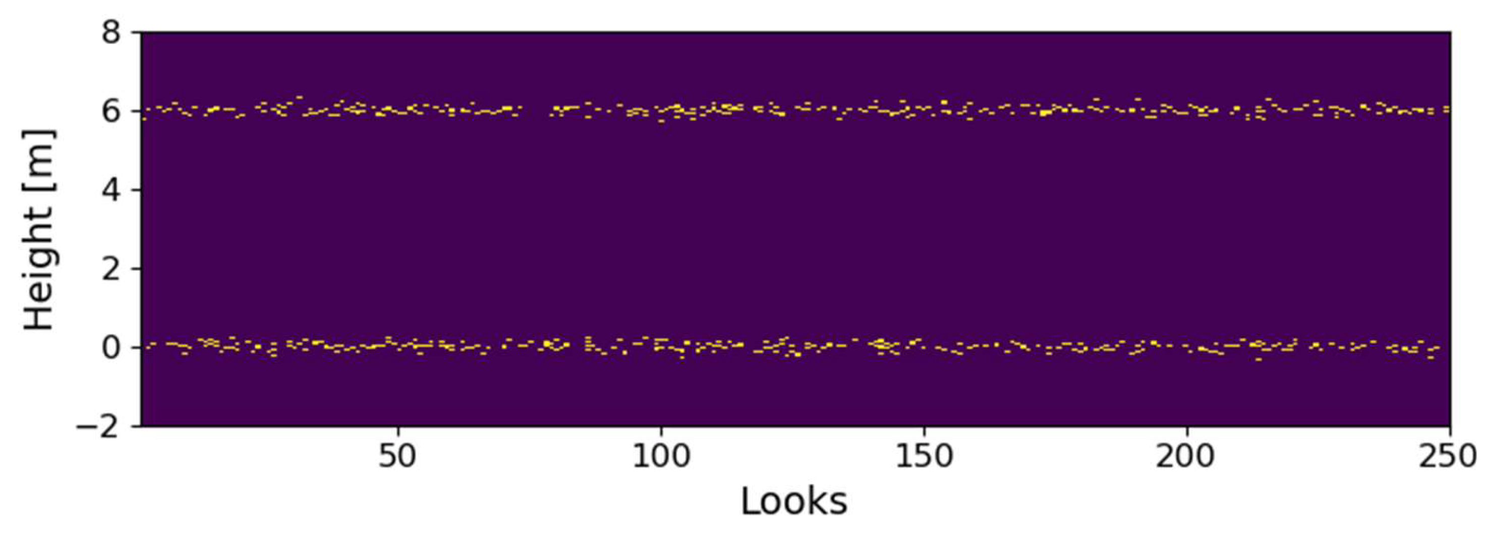
In order to demonstrate the performance of the novel WAVAB approach in comparison to the previously mentioned competing techniques, the signals of two uncorrelated scatterers with equal reflectivity are simulated. To simulate independent realizations of the data vector
in (1), we consider that the two scatterers follow (for simplicity) two Gaussian distributions among
independent looks, with phase-centers (means) located at
m and
m, respectively, and spread (standard deviation)
m, as depicted in
Figure 2.
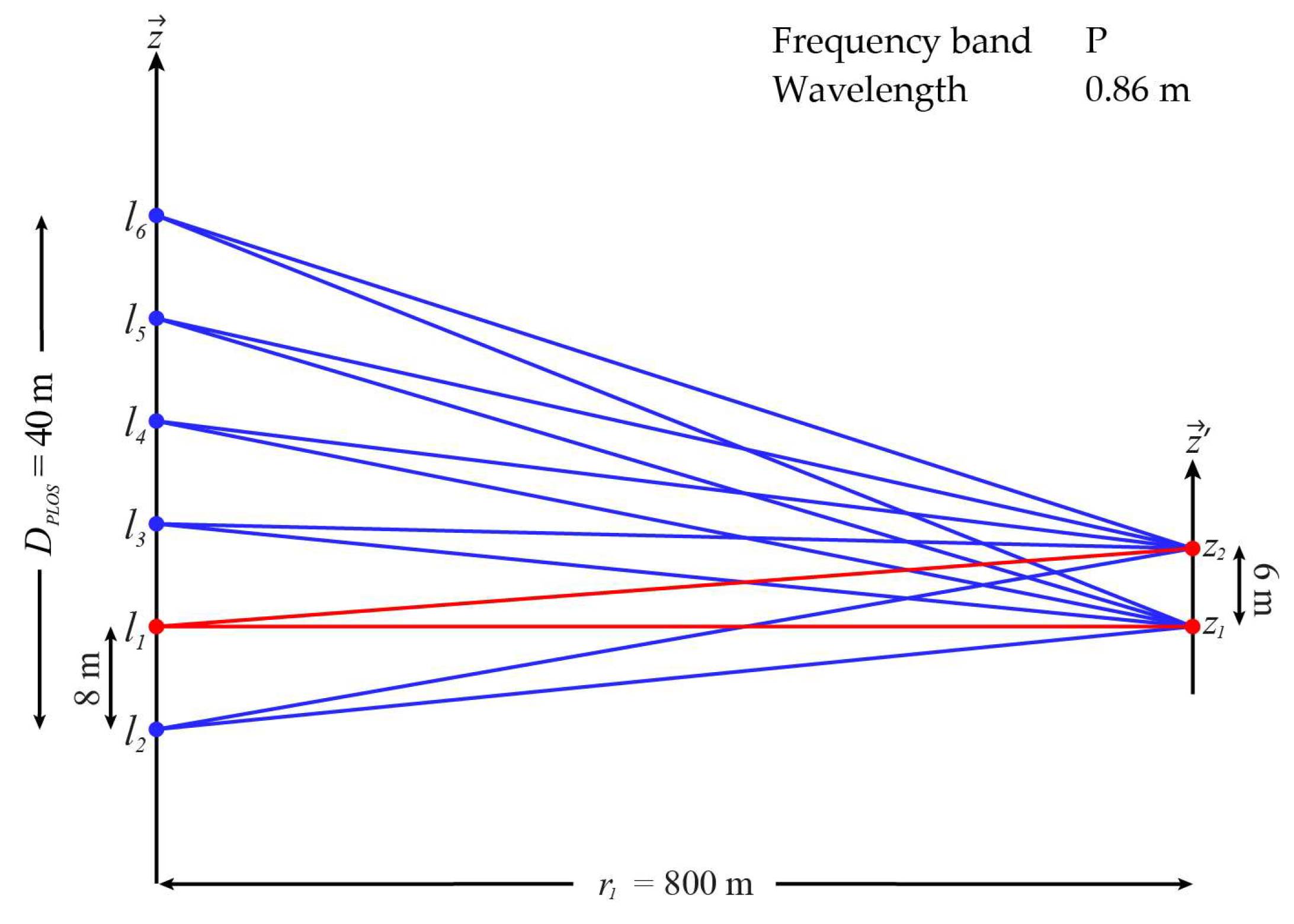
Also, we consider a P-band sensor with wavelength
m and the simplified tomographic acquisition geometry shown in
Figure 3, composed of
L = 6 PLOS-oriented tracks with baselines evenly distributed, spanning a synthetic aperture of
m. The first target
is assumed to be at a slant-range distance from the master track of
m, meaning a Fourier resolution,
[
2], of 8.6 m in the PLOS direction.
In the simulations reported next, we calculate the mean squared error (MSE)
between the actual positions
and the retrieved estimates
, for each particular case, using 100 Monte-Carlo trials, with the aim of obtaining the average value. As in (21),
refers to the respective phase-center.
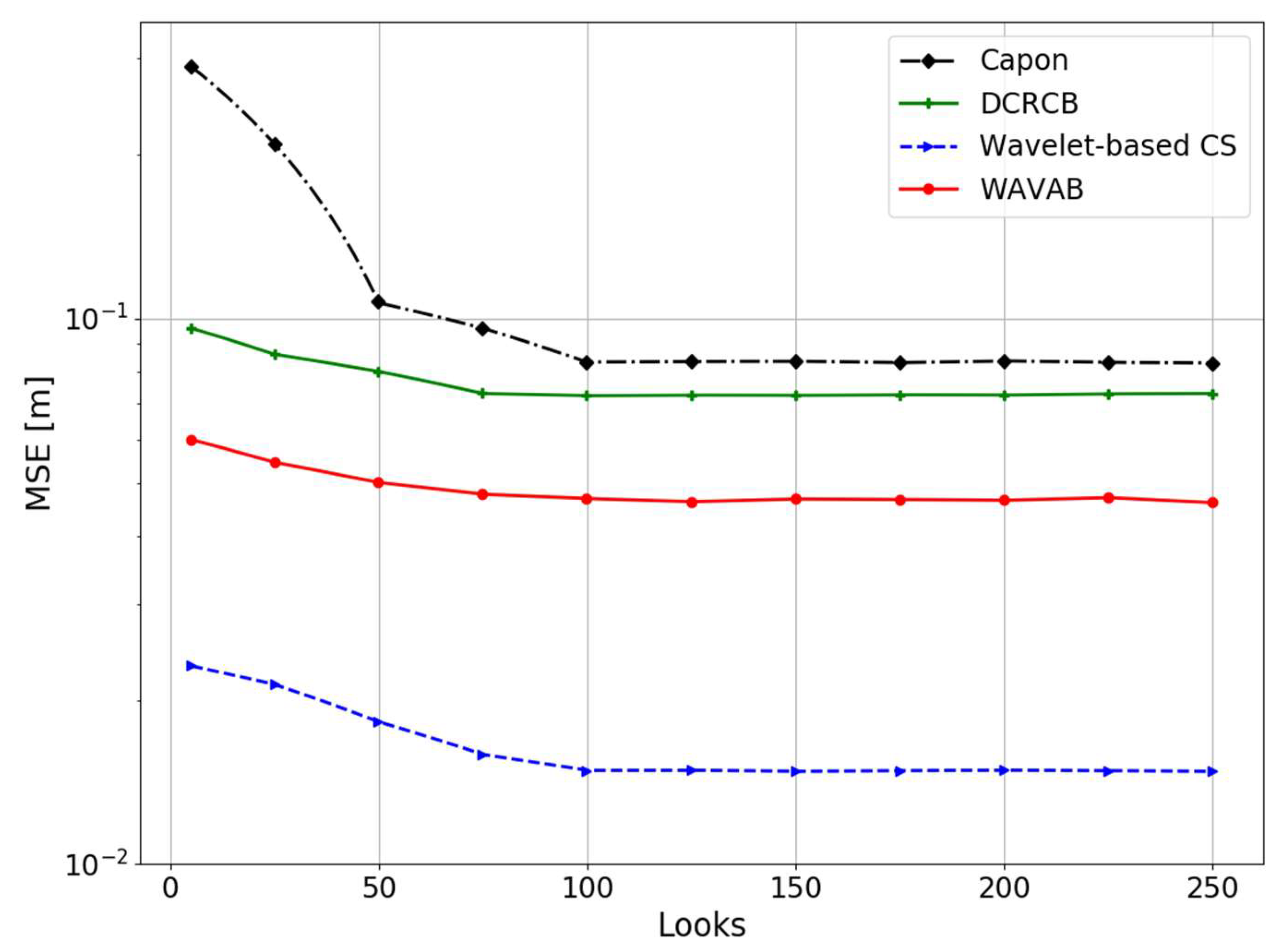
First, we simulate the data covariance matrix
in (10), with different number of looks
J, in order to investigate the asymptotic properties of the Capon, DCRCB, CS and WAVAB techniques. The power spectral density of the white noise power is set to
= 0.01.
Figure 4 shows the fast convergence properties of the aforementioned focusing techniques to a lower MSE as the number of looks increases. The Capon and DCRCB methods converge to almost the same value, whereas WAVAB and CS converge to a minor MSE, CS being the technique with better performance. As expected, due to the involved inversion of the data covariance matrix
, Capon presents worse results for a low number of looks, being inapplicable when matrix
is rank deficient (
).
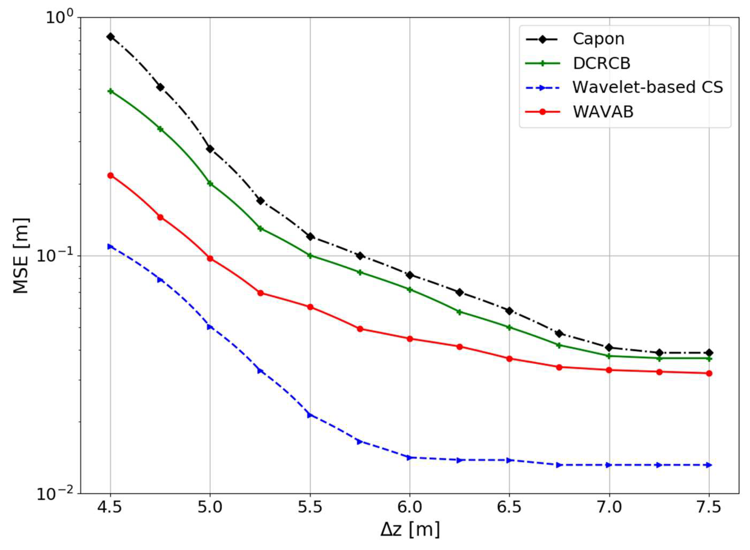
In order to study the vertical resolution, a different distance between scatterers,
, is simulated. We consider that the first target
stays at the same location and a high multi-looking value of
.
Figure 5 depicts how the accuracy of all methods improves as
increases. We can notice that the Capon, DCRCB and WAVAB techniques provide similar MSE when
approaches to the Fourier resolution, while, in general, CS provides more accurate estimates than the other competing methods. On the other hand, for smaller distances between scatterers
, the WAVAB estimator retrieves better results than Capon and DCRCB.
Typically, when a high number of looks J is considered, both Capon and DCRCB estimators tend to have similar responses. When the data covariance matrix results in being rank deficient, the use of the robust versions of Capon beamforming, as DCRCB, is recommended. For the particular case of SKP decomposition, multi-looking is performed first in the MP-MB data covariance matrix (22) to handle multiple non-deterministic sources; thus, to prevent resolution loss, it is advisable to avoid a second multi-looking procedure in the retrieved (rank-deficient) structure matrices; rather, robust methods as DCRCB, CS and the novel WAVAB are employed.
The next sections are intended to corroborate the capabilities of the introduced WAVAB approach through experimental results, and to point out its particular advantages in comparison to the other competing approaches. First, in order to study the robustness of the methods against irregular sampling, the tomographic slices of a forested test site are retrieved, using a non-evenly distributed acquisition constellation. Then, in order to analyze the response of the methods using only a few available snapshots, the SKP decomposition technique is applied at the pre-processing stage, retrieving rank-deficient structure matrices. A second multi-looking procedure is not performed with the aim of preserving resolution.
7. Experimental Results
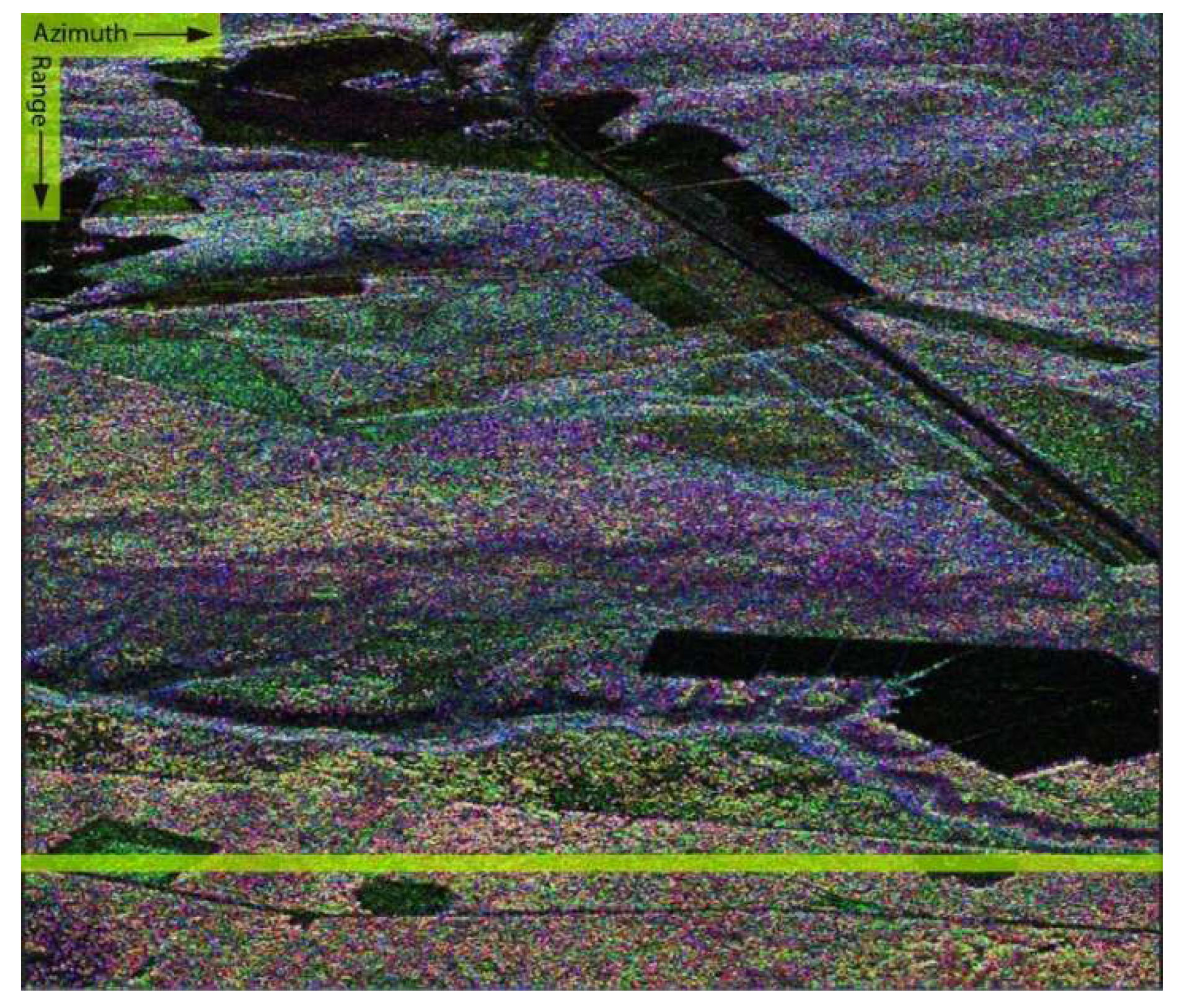
To demonstrate the enhanced imaging capabilities of the multi-stage TomoSAR WAVAB technique (19), (20), we use a stack of nine single-look complex SAR images properly co-registered and phase flattened (
Figure 6 shows one image out of the stack), obtained by processing fully polarimetric P-band data of the German Aerospace Center (DLR), acquired by the E-SAR airborne sensor, during the BioSAR campaign in October 2008, in the forested test area located at the Vindeln municipality, in northern Sweden. The main parameters of the E-SAR sensor, used during the BioSAR 2008 campaign, are gathered in
Table 1.
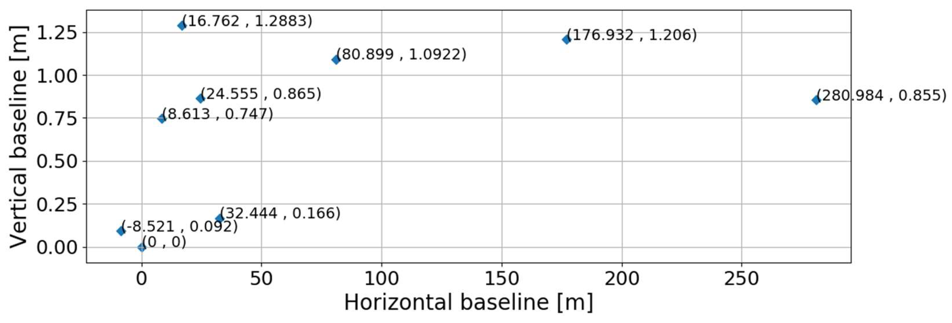
Phase calibration has been performed by exploiting the availability of permanent scatterers, namely, single-stable targets within the illuminated scene [
26]. The acquisition constellation follows the minimum redundancy principle [
27], spanning a horizontal synthetic aperture of approximately
m, as shown in
Figure 7. In practice, regions with high air traffic, such as the one considered in this study, demand to operate over only one height level, so that the flight space is not blocked. Therefore, the acquisition constellation rather spans a horizontal synthetic aperture
.
The tomographic reconstruction has been conducted as follows: several azimuth positions at a fixed range distance were selected as indicated by the yellow rectangle in
Figure 6. The tomographic slices in the azimuth and height PLOS directions correspond to 1080 m by 40 m acquisition formats.
For the selected range line, with incidence angle
° and slant-range distance
m, the Fourier resolution,
[
28], is about 12 m (
stands for the look angle). However, due to the irregular sampling, it is expected to have high ambiguity levels.
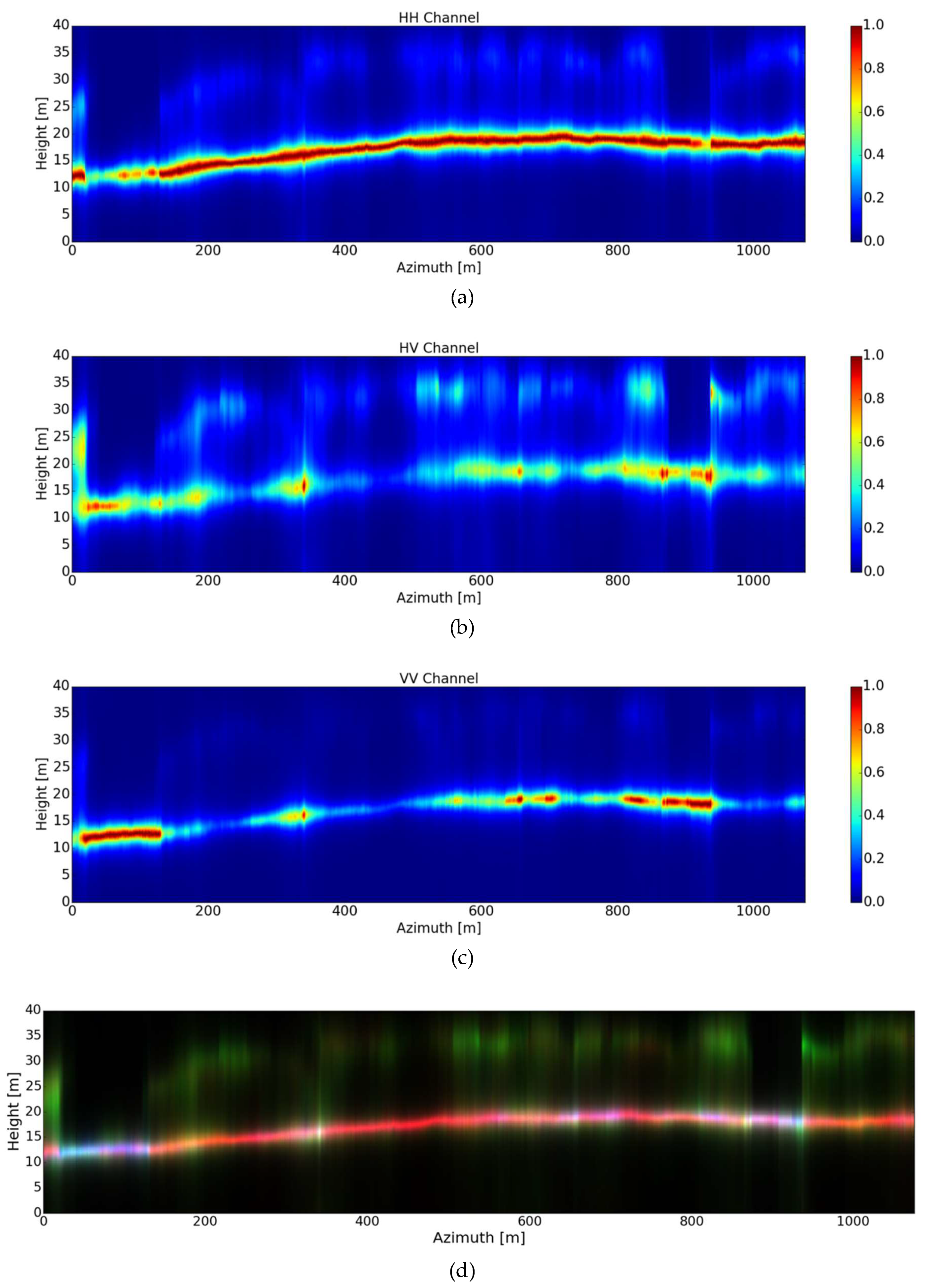
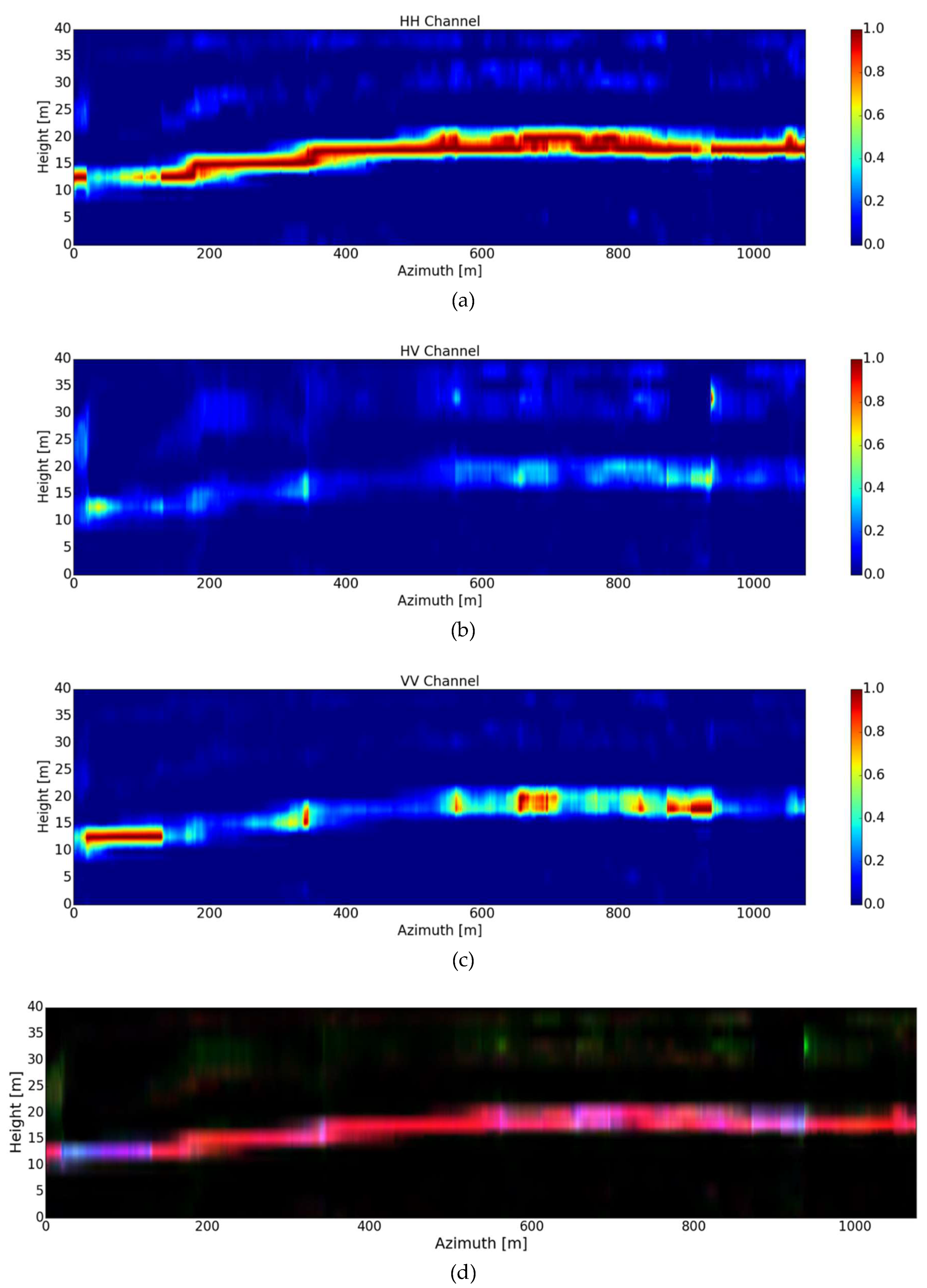
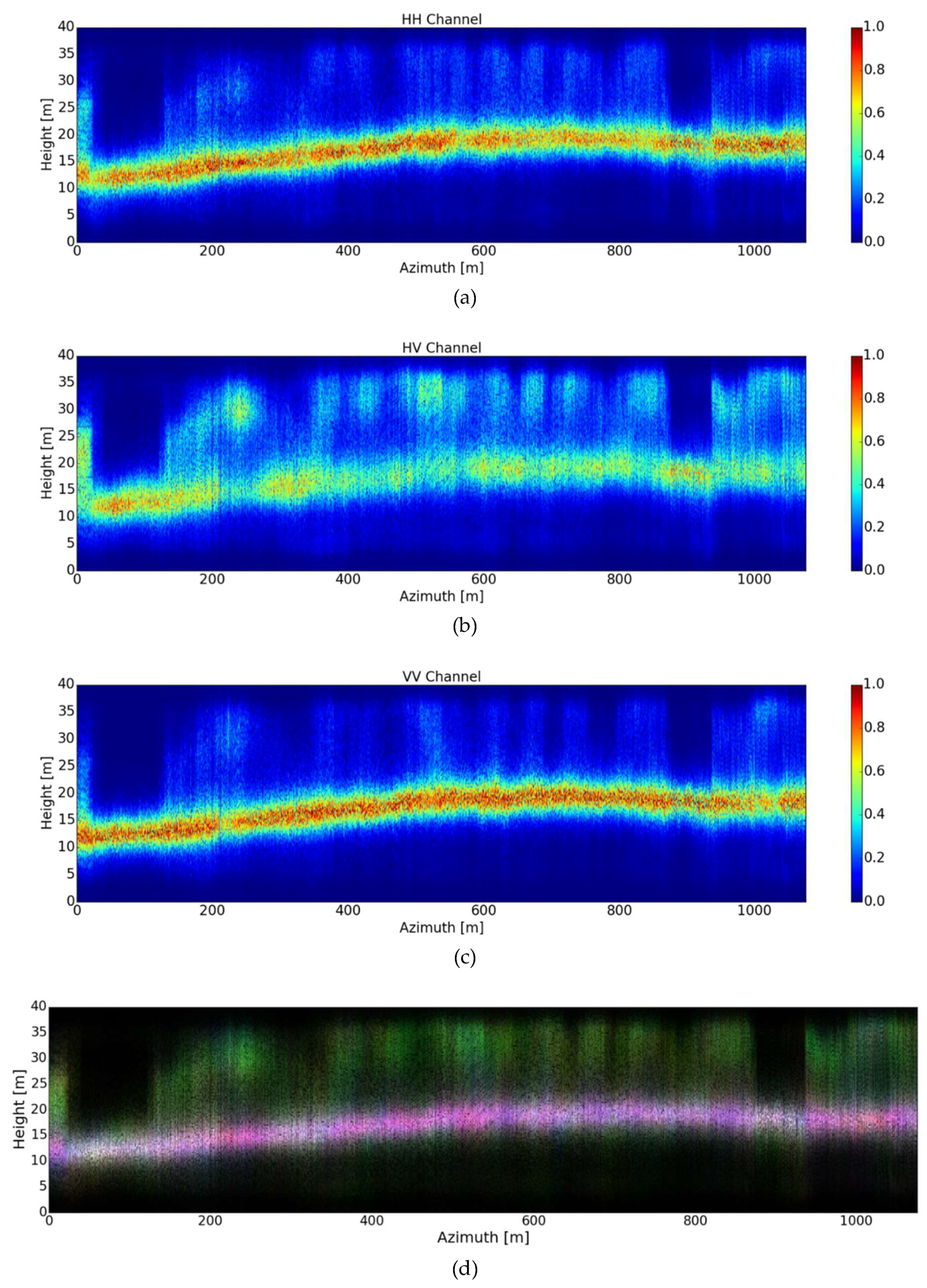
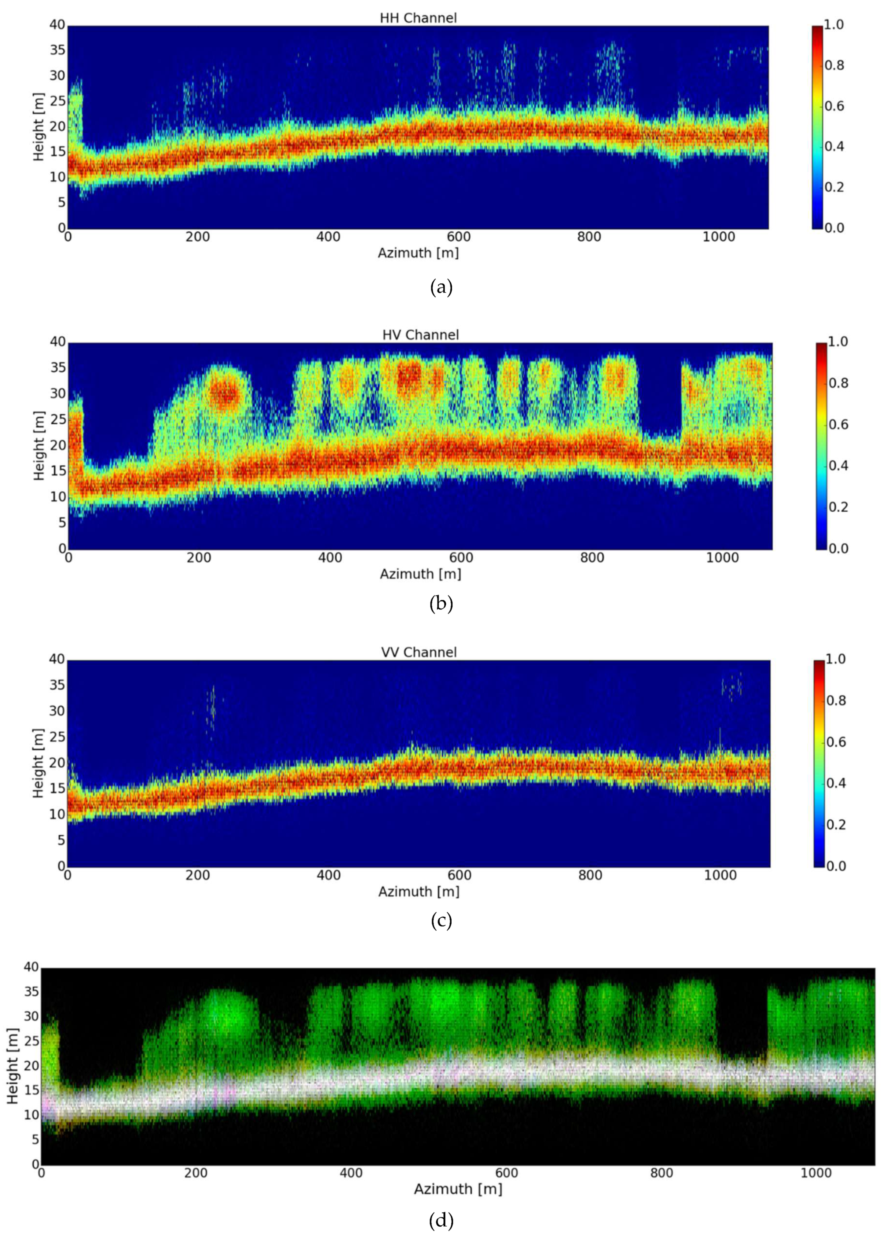
Figure 8,
Figure 9,
Figure 10,
Figure 11,
Figure 12 and
Figure 13 show the recovered tomographic slices for the selected azimuth positions at the specified range line (refer to
Figure 6), using the MSF, Capon beamforming, DCRCB, CS and WAVAB approaches, correspondingly, for each polarization. The tomograms retrieved by means of the introduced TomoSAR WAVAB method at the first DEDR-VAB stage (19), with convergence at
I = 8 iterations, are shown in
Figure 12; while the tomograms recovered after the second WDT stage (20), followed by
T = 3 iterations (in total 11 iterations), are depicted in
Figure 13.
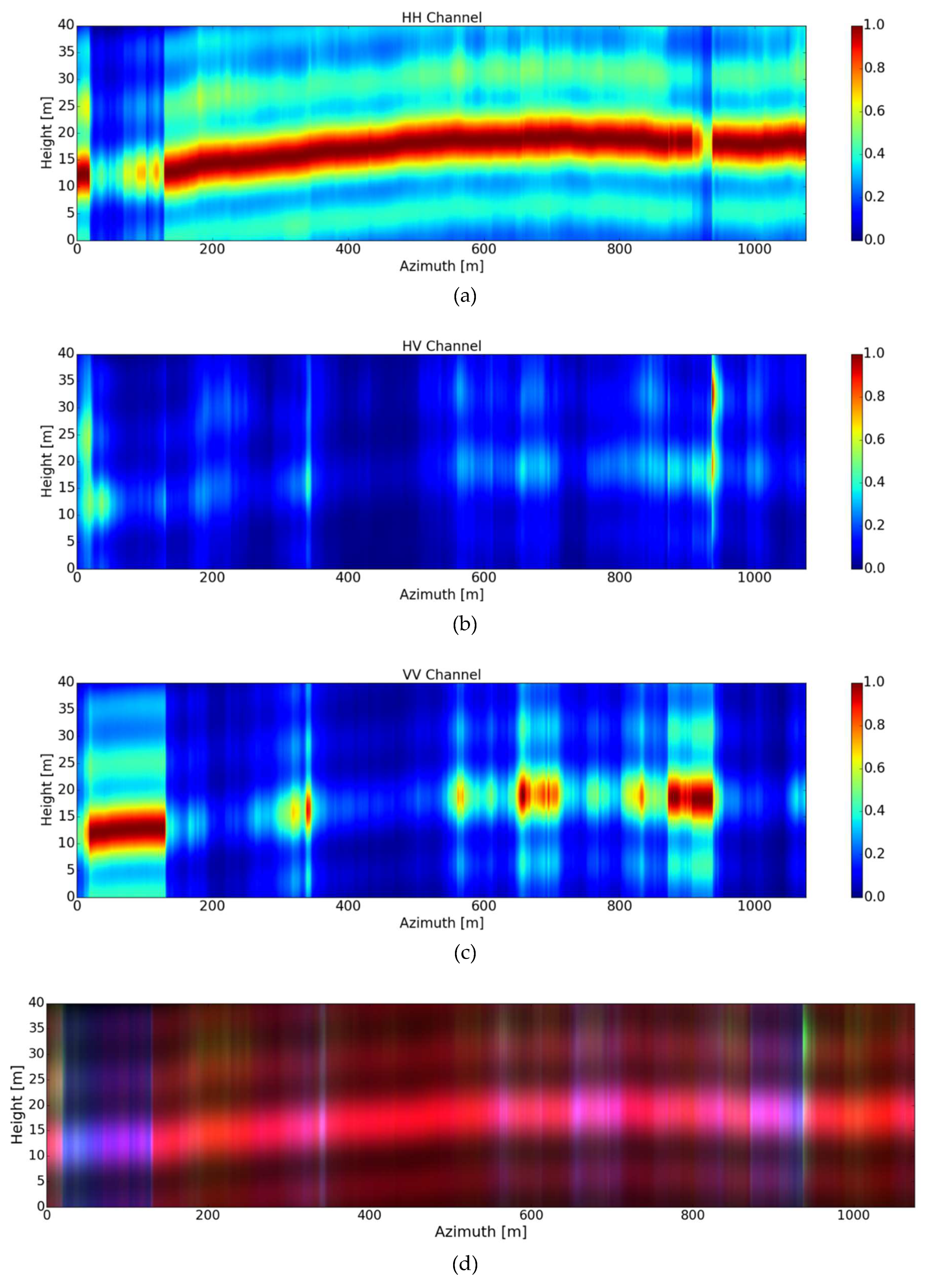
For all cases, the color coded tomogram, calibrated to the same [0,1] scales, for the three corresponding polarimetric channels (red
HH, green
HV and blue
VV) is also presented. The employed wavelet-based CS technique considers a sparsifying basis based on the Symlets 4 wavelet family with three decomposition levels, as suggested in the previous related studies [
8,
9].
Next, the SKP decomposition technique is applied on the measured MP-MB data covariance matrix (22) at the pre-processing stage, retrieving the (rank-deficient) structure matrices for both ground-only and canopy-only contributions. Since the ground component behaves as a point-type target [
15,
16], its tomogram is recovered using the multiple signal classification (MUSIC) method [
3,
7] with a single source model (as shown in
Figure 14), which is better suited for such kinds of responses. On the other hand, the canopy-only contributions are treated using TomoSAR focusing techniques that are better adapted to tackle with volumetric targets, including the proposed WAVAB approach. The conventional Capon beamforming method [
3,
7] is usually not used, due to the ill-posed nature of the involved structure matrix inversion; rather, the DCRCB technique [
24,
25] is used instead, which overcomes the aforementioned limitation.
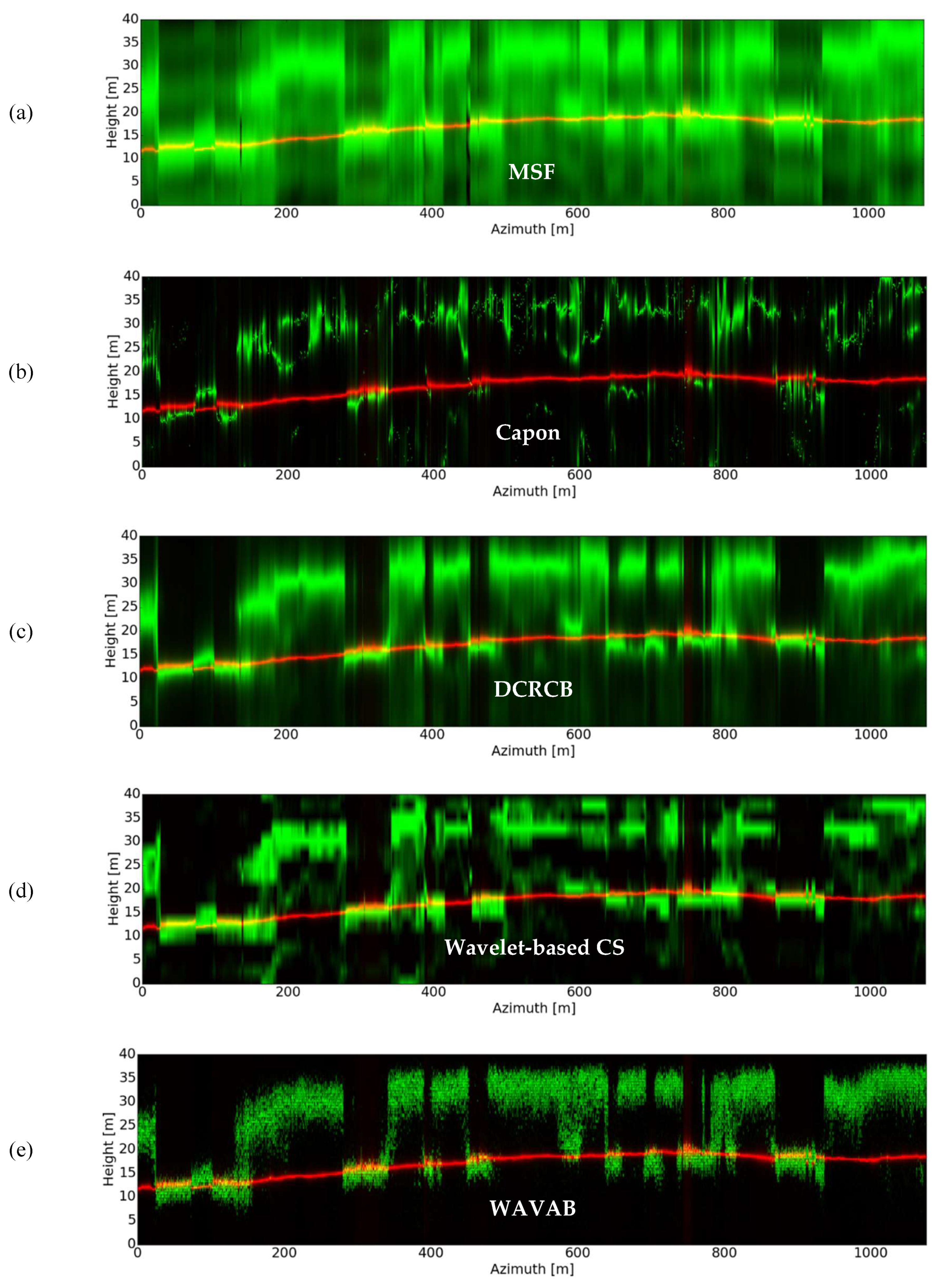
Figure 14 presents then a comparison between the reconstructed canopy-only tomograms by means of the related most prominent competing techniques: (a) MSF beamforming; (b) Capon beamforming; (c) DCRCB; (d) wavelet-based CS; followed by the outlined (e) WAVAB approach in (19), (20). The average processing time of the addressed TomoSAR focusing techniques (with SKP decomposition at the pre-processing stage) needed to retrieve the canopy-only tomograms, is presented in
Table 2.
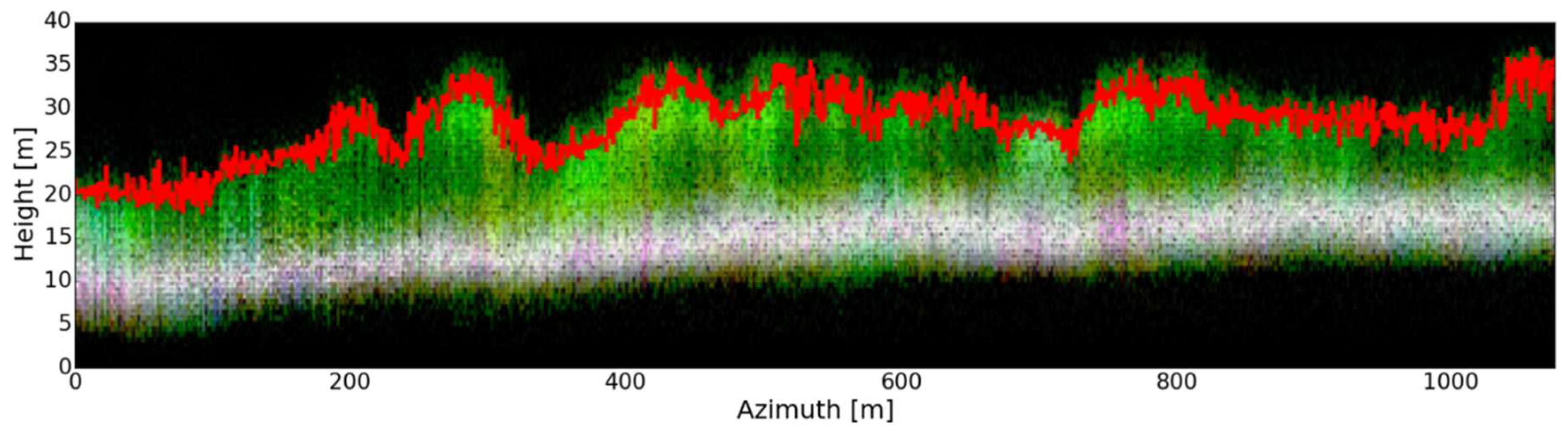
Finally, we compare the recovered phase-center locations of the novel WAVAB approach against the retrieved phase-center locations of the well-established DCRCB method [
24,
25] through the computation of the MSE (24) between both estimates. The aim of this comparison is to show how consistent the results of the WAVAB technique are with respect to the well-known DCRCB technique. To calculate the MSE, we consider each azimuth position among a set of 50 different range lines within the considered test site (
Figure 6), for which, the computed MSE equals 0.26 m. The reason to choose DCRCB for this comparison is due to the similarity between methods, treated both, by constructions, as a refinement of Capon beamforming, being robust with respect to non-regular constellation geometries and only few available looks.
Figure 15 shows the contour of the top of the canopy (red), retrieved from the DCRCB phase-center estimates at the highest position, superimposed on a tomogram obtained using WAVAB, for a certain range line out of the set of 50.
8. Discussion
From the assessed experiments, we can observe that, as expected, the conventional DOA-inspired MSF beamforming technique [
3] (
Figure 8) presents high ambiguity levels, mostly due to the irregular sampling and due to the reduced number of passes; the latter complicates the accurate location of the ground and canopy phase centers. Incorporation of the SKP decomposition technique [
15,
16] at the pre-processing stage of all addressed TomoSAR imaging procedures (
Figure 14) evidences considerable improvement on ground and canopy separation, allowing the utilization of a better suited TomoSAR technique, as MUSIC [
3,
7], on the ground structural components, which tend to behave as a point-type target. Yet, for the particular case of MSF beamforming, the presence of high ambiguity levels remains after SKP decomposition, as it can be observed in
Figure 14a.
The SKP decomposition technique is a parametric approach that expects to have contributions from both ground-only and canopy-only effective SMs. Therefore, in areas without vegetation, the two corresponding tomograms superimpose each other (refer to
Figure 14).
Capon beamforming [
3,
7] performs better than the MSF technique for the considered irregularly distributed acquisition constellation (refer to
Figure 7), as it can be seen in
Figure 9. It provides enhanced resolution and lower ambiguity levels in comparison to MSF. On the other hand, since the retrieval of rank-deficient structure matrices is common after SKP decomposition, Capon beamforming presents in such case a poor performance due to the ill-posedness of the involved structure matrix inversion, as depicted in
Figure 14b.
The formation of the MP-MB covariance matrix in (22) involves multi-looking in order to handle multiple non-deterministic sources. A second multi-looking procedure on the retrieved structure matrices, after SKP separation, is usually avoided in order to prevent resolution loss. Rather, the use of robust versions of the conventional Capon beamforming method, such as the DCRCB approach [
24,
25], is recommended, which alleviates the drawback related to the cumbersome inversion of the recovered rank-deficient structure matrices.
We can observe through
Figure 14c, that after the SKP pre-processing stage, DCRCB performs better than Capon beamforming when only few snapshots (looks) are available. However, the presence of artifacts and high ambiguity levels is still an issue. Also, DCRCB demands more processing time in contrast to the standard MSF and Capon beamforming techniques, as depicted in
Table 2, due to the use of numerical methods to recover the involved Lagrange multipliers and due to the eigen-decomposition of the structure matrices.
Consistently with the previously addressed numerical examples, the wavelet-based CS approach [
8,
9] (
Figure 11) provides finer resolution in comparison to the other competing techniques, including the introduced WAVAB approach. This is especially notorious in
Figure 14d, after SKP decomposition, where we can observe the detection of multiple vegetation layers (phase centers) among the canopy. The wavelet-based CS method is also robust against the presence of only few available looks; however, due to the iterative nature of the method and due to the non-availability of adapted efficient convex optimization algorithms, it incurs much more computation time in contrast to the other addressed competing techniques (refer to
Table 2). In this study, the CVXPY software library [
29] has been employed to solve the involved convex optimization problem. Furthermore, the main drawback of CS is related to the presence of artifacts and high ambiguity levels after focusing; particularly, the introduction of artifacts is usually translated into false detections, which complicate the discrimination of the actual ground and canopy phase centers.
The first stage of the novel WAVAB estimator is presented in
Figure 12, which relates to the DEDR-inspired solutions in (19). At this stage, we can notice the retrieval of detailed height profiles reconstructions with lower ambiguity levels. Later on, the WDT-based second stage (20) is shown in
Figure 13, which provides additional image enhancement, with suppression of artifacts, to the previously recovered DEDR-inspired estimates. The balance between information lost and suppression of artifacts is controlled via modifying the Donoho’s soft thresholding shrinkage parameter
in (20), when
is not properly set some information may be lost [
13].
The introduced WAVAB technique performs consistently with the other addressed TomoSAR-adapted non-parametric methods. The reliability of the retrieved estimates is corroborated through the comparison of the canopy-only tomograms in
Figure 14, where we can notice the tendency of all methods to follow the same outline along azimuth.
Figure 15 also shows how consistent the WAVAB approach is against the well-established DCRCB method, through the comparison of the retrieved phase-center location estimates. The reason to choose DCRCB for this evaluation is due to the similarity between methods, both treated by constructions as a refinement of Capon beamforming.
By definition, the WAVAB technique in (19) depends on a first estimate of the PSP, which acts as first input (zero-step iteration). For such purpose, the MSF beamforming technique is used. Therefore, the degradation or improvement of the solver depends on the precision of the first estimate, meaning that the solution degrades or improves depending on the accuracy of the MSF estimates.
The main characteristics of the WAVAB technique are summarized as follows: (i) It is robust with respect to irregularly distributed acquisition geometries, such as the one considered in this study, presented in
Figure 7; (ii) it is robust against the few available snapshots, meaning that it can be applied on the rank-deficient structure matrices retrieved after SKP separation of ground and canopy; (iii) its processing time is comparable to DCRCB and is significantly lower than wavelet-based CS, as depicted in
Table 2; (iv) it achieves better suppression of artifacts and ambiguity levels reduction in contrast to the other assessed techniques, as observed in
Figure 13 and
Figure 14e, easing the localization of the recovered (estimated) ground and canopy phase centers and preventing false detections; and (v) it performs consistently with the other addressed competing techniques.


