Comparison of Aerosol Reflectance Correction Schemes Using Two Near-Infrared Wavelengths for Ocean Color Data Processing

Abstract

This paper reanalyzes the aerosol reflectance correction schemes employed by major ocean color missions. The utilization of two near-infrared (NIR) bands to estimate aerosol reflectance in visible wavelengths has been widely adopted, for example by SeaWiFS/MODIS/VIIRS (GW1994), OCTS/GLI/SGLI (F1998), MERIS/OLCI (AM1999), and GOCI/GOCI-II (A2016). The F1998, AM1999, and A2016 schemes were developed based on GW1994; however, they are implemented differently in terms of aerosol model selection and weighting factor computation. The F1998 scheme determines the contribution of the most appropriate aerosol models in the aerosol optical thickness domain, whereas the GW1994 scheme focuses on single-scattering reflectance. The AM1999 and A2016 schemes both directly resolve the multiple scattering domain contribution. However, A2016 also considers the spectrally dependent weighting factor, whereas AM1999 calculates the spectrally invariant weighting factor. Additionally, ocean color measurements on a geostationary platform, such as GOCI, require more accurate aerosol correction schemes because the measurements are made over a large range of solar zenith angles which causes diurnal instabilities in the atmospheric correction. Herein, the four correction schemes were tested with simulated top-of-atmosphere radiances generated by radiative transfer simulations for three aerosol models. For comparison, look-up tables and test data were generated using the same radiative transfer simulation code. All schemes showed acceptable accuracy, with less than 10% median error in water reflectance retrieval at 443 nm. Notably, the accuracy of the A2016 scheme was similar among different aerosol models, whereas the other schemes tended to provide better accuracy with coarse aerosol models than the fine aerosol models.

1. Introduction

In the last few decades, ocean observations using visible (VIS) to near-infrared (NIR) wavelength satellite imagery have successfully retrieved oceanic environmental information over a large spatial and temporal range [1,2,3,4,5,6,7,8]. Atmospheric correction is a primary process in satellite ocean color missions, in which surface water reflectance, ρ_wn, is extracted from the top of atmosphere (TOA). The quantity of ρ_wn is generally less than 10% of the TOA reflectance (ρ_TOA); thus, atmospheric reflectance and transmittance should be computed as accurately as possible. Ignoring the surface-reflectance from sun-glint and whitecaps, ρ_TOA at each wavelength (λ) can be described as follows [9,10]:

$${\rho }_{\mathrm{TOA}}={\rho }_r+{\rho }_a+{\rho }_{ra}+t_d^s{t}_d^v{\rho }_{wn}$$

(1)

where ρ_r is the Rayleigh multiple-scattering (molecular multiple-scattering) reflectance in the absence of aerosols, and ρ_a + ρ_ra is the aerosol multiple-scattering reflectance in the presence of air molecules (denoted ρ_am). Terms t^s_d and t^v_d are the diffuse transmittances of the atmosphere from the sun to the sea surface and from the sea surface to the sensor, respectively.

Traditional atmospheric correction processes first compute ρ_r(λ) within 1% error using a radiative transfer simulation [11,12,13,14,15]. Following subtraction of the Rayleigh reflectance contribution, ρ_am(NIR) can be estimated by assuming that the NIR water-leaving reflectance is negligible, i.e., ρ_wn(NIR) = 0, due to the relatively strong light absorption of the waterbody or so-called “black pixel” assumption. ρ_am(VIS) is then extrapolated from satellite-observed ρ_am(NIR) by inversion of the radiative transfer simulation.

The inverse processes for aerosol correction are generally separated into two steps: aerosol model selection, and subsequent spectral extrapolation of ρ_am(VIS) from ρ_am(NIR). In the model selection step, two similar aerosol models, and the contributions of their weighting factors, are extrapolated from ρ_am(NIR). ρ_am(VIS) is then computed from ρ_am(NIR) using the aerosol information estimated in the extrapolation step.

Various inverse schemes using two-NIR bands have been developed for ocean color missions, including the SeaWiFS/MODIS/VIIRS scheme [9,10] (denoted GW1994), OCTS/GLI/SGLI scheme [16,17] (denoted F1998), MERIS/OLCI scheme [18,19] (denoted AM1999), and GOCI/GOCI-II scheme [20] (denoted A2016). Schemes F1998, AM1999, and A2016 were developed theoretically based on GW1994 and the aerosol model selection and spectral extrapolation are slightly different.

Schemes GW1994, F1998, and AM1999, but not A2016, were compared and evaluated for a coarse maritime aerosol model with a relative humidity (RH) of 80%, and presented in a report by the International Ocean Colour Coordinating Group (IOCCG) [21]. However, the IOCCG comparison focused more on differences in atmospheric correction systems than on differences of the aerosol correction schemes. Since each scheme used different aerosol models and different radiative transfer code and different Mie scattering code, it is difficult to determine which factors account for the different performances between the schemes.

In this paper, we first revisit and compare the above-mentioned schemes, including the A2016 scheme, and then present our results, in which the performance of each algorithm was examined using a simulated TOA dataset generated by radiative transfer simulations [22,23,24]. Our analysis was performed using aerosol models with a size distribution including fine to coarse aerosols, whereas the IOCCG study only looked at coarse aerosols in their models. For clarification of the comparison, we used the same code and model for the radiative transfer, Mie scattering calculations, and aerosol models for both the implementation and the analysis result.

2. The Two-NIR Aerosol Correction Methods Used by the Various Schemes

This section describes various two-NIR aerosol correction schemes. The correction schemes and look-up tables were developed simultaneously to allow comparison (as summarized in

Table 1. Aerosol reflectance correction schemes based on the black pixel assumption.

Method	References	Applied Sensors	Aerosol Model Selection Domain
GW1994	[9,10]	SeaWiFS, MODIS, VIIRS	Single-scattering
F1998	[16,17]	OCTS, GLI, SGLI	Aerosol optical thickness
AM1999	[18,19]	MERIS, OLCI	Multiple-scattering
A2016	[20]	GOCI, GOCI-II	Multiple-scattering

). Fundamentally, F1998, AM1999, and A2016 were developed based on GW1994; the principle differences between the listed schemes lie in the details of the aerosol model and weighting factor determination. Specifically, the GW1994 scheme uses the spectral ratio of the aerosol single-scattering reflectance of two NIR bands, and the F1998 scheme uses the spectral ratio of the aerosol optical thickness (τ_a) of two NIR bands}. Both the AM1999 and A2016 schemes apply the spectral ratio of aerosol multiple-scattering reflectance of two NIR bands; however, A2016 is slightly modified to consider the spectrally varying weighting factor [19,20]. In the AM1999 scheme, the path reflectance increment ratio term (ρ_am + ρ_r)/ρ_r by aerosol concentration is utilized, whereas other schemes use ρ_am.

2.1. GW1994 Scheme

The GW1994 scheme determines aerosol model contributions in the single-scattering domain. Therefore, GW1994 first converts ρ_am into single-scattering aerosol reflectance (ρ_as) for two NIR bands (hereafter, the shorter wavelength NIR band is denoted by NIR_S, and the longer wavelength NIR band is denoted by NIR_L) for all i-th candidate aerosol models (M_i), as follows:

$${\rho }_{as}(M_i,\lambda ,\Theta )=F_{m\to s}({\rho }_{am},M_i,\lambda ,\Theta )$$

(2)

where F_m→s is the empirical function for converting ρ_as to ρ_am for specific λ, M_i, and Θ. The Θ is the scanning geometry variable that is a combination of solar zenith angle, satellite zenith angle, and relative azimuth angle values [9,10,21,25].

ρ_as values are then used to calculate the single-scattering reflectance ratio (ε_as), used for selecting the appropriate aerosol models from among the candidate models (M_i):

$${\epsilon }_{as}(M_i,{\mathrm{NIR}}_{\mathrm{S}},{\mathrm{NIR}}_{\mathrm{L}},\Theta )={\rho }_{as}(M_i,{\mathrm{NIR}}_{\mathrm{S}},\Theta )/{\rho }_{as}(M_i,{\mathrm{NIR}}_{\mathrm{L}},\Theta )$$

(3)

Each M_i has a theoretical eigenvalue of ε_as (denoted as ε^M_as) derived from the analytical single-scattering reflectance model, determined by the single-scattering albedo of M_i and the phase function. The GW1994 scheme selects two similar aerosol models, M_L and M_H, by comparing the representative ε_as (denoted as ε^r_as) to ε^M_as, as follows:

$${\epsilon }_{as}^{\mathrm{M}}(M_{\mathrm{L}},{\mathrm{NIR}}_{\mathrm{S}}{,\mathrm{NIR}}_{\mathrm{L}},\Theta )\le {\epsilon }_{as}^r({\mathrm{NIR}}_{\mathrm{S}}{,\mathrm{NIR}}_{\mathrm{L}},\Theta )<{\epsilon }_{as}^{\mathrm{M}}(M_{\mathrm{H}},{\mathrm{NIR}}_{\mathrm{S}}{,\mathrm{NIR}}_{\mathrm{L}},\Theta )$$

(4)

The representative ε_as(NIR_S, NIR_L) can be approximated by averaging over the ε^M_as of all candidate models, as the conversion function F_m→s is less sensitive to the aerosol model for NIR wavelengths:

$${\epsilon }_{as}^r({\mathrm{NIR}}_{\mathrm{S}}{,\mathrm{NIR}}_{\mathrm{L}},\Theta )\approx \frac{1}{N}{\displaystyle \sum _{i=1}^N{\epsilon }_{as}^{}(M_i,{\mathrm{NIR}}_{\mathrm{S}}{,\mathrm{NIR}}_{\mathrm{L}},\Theta )}$$

(5)

Then, the weighting factors $w^{M_{\mathrm{L}}}$ and $w^{M_{\mathrm{H}}}$ for the two selected aerosols (M_L and M_H) can be estimated by the fraction of the linear distance between ε^r_as and ε^M_as:

$$w^{M_{\mathrm{H}}}=\frac{{\epsilon }_{as}^r({\mathrm{NIR}}_{\mathrm{S}}{,\mathrm{NIR}}_{\mathrm{L}},\Theta )-{\epsilon }_{as}^{\mathrm{M}}(M_{\mathrm{L}},{\mathrm{NIR}}_{\mathrm{S}}{,\mathrm{NIR}}_{\mathrm{L}},\Theta )}{{\epsilon }_{as}^{\mathrm{M}}(M_{\mathrm{H}},{\mathrm{NIR}}_{\mathrm{S}}{,\mathrm{NIR}}_{\mathrm{L}},\Theta )-{\epsilon }_{as}^{\mathrm{M}}(M_{\mathrm{L}},{\mathrm{NIR}}_{\mathrm{S}}{,\mathrm{NIR}}_{\mathrm{L}},\Theta )},$$

(6)

$$w^{M_{\mathrm{L}}}=1-w^{M_{\mathrm{H}}}$$

(7)

The ρ_as(VIS) for the two selected models can be extrapolated spectrally from ρ_as(NIR) based on ε^M_as(NIR, VIS). Having derived the values $w^{M_{\mathrm{L}}}$ and $w^{M_{\mathrm{H}}}$ for M_L and M_H, respectively, the aerosol multiple-scattering reflectance (ρ_am) in the VIS bands is given by:

$${\rho }_{am}(\lambda ,\Theta )=w^{M_{\mathrm{L}}}{F}_{s\to m}\left({\rho }_{as},M_{\mathrm{L}},\lambda ,\Theta \right)+w^{M_{\mathrm{H}}}{F}_{s\to m}\left({\rho }_{as},M_{\mathrm{H}},\lambda ,\Theta \right)$$

(8)

where F_s→m is the inverse function of F_m→s [9,10,21,25].

2.2. F1998 Scheme

The F1998 scheme determines the contributions of the aerosol models to the τ_a domain [16], and has the advantage that the model-wise single-scattering reflectance ratios are often unevenly distributed over the single-scattering space [26]. For model determination, F1998 uses the inter-band τ_a ratio of two NIR bands, as follows:

$${\epsilon }_{\tau a}^{}(M_i,{\mathrm{NIR}}_{\mathrm{S}},{\mathrm{NIR}}_{\mathrm{L}})={\tau }_a^{}(M_i,{\mathrm{NIR}}_{\mathrm{S}})/{\tau }_a^{}(M_i,{\mathrm{NIR}}_{\mathrm{L}})$$

(9)

where ε_τa is the ratio of τ_a of two wavelengths.

Therefore, the F1998 scheme first converts ρ_am into τ_a for all candidate models, M_i, using an empirical conversion function (F_m→τ) between ρ_am and τ_a, in contrast to Equation (2), as follows:

$${\tau }_a^{}(M_i,\lambda )=F_{m\to \tau }({\rho }_{am},M_i,\lambda ,\Theta )$$

(10)

The F_m→τ function can be expressed in several ways [18,19,27,28], and F1998 uses a third-order polynomial function to describe the empirical relationship [16].

Theoretically, each M_i has a scan geometry-independent eigenvalue of ε^M_τa that can be expressed by the ratio of the aerosol extinction coefficient K_ext(M_i, λ), as follows:

$${\epsilon }_{\tau a}^{\mathrm{M}}(M_i,{\lambda }_1,{\lambda }_2)=\frac{K_{ext}(M_i,{\lambda }_1)}{K_{ext}(M_i,{\lambda }_2)}$$

(11)

In a similar way to Equation (4), the contributions of M_L and M_H can be determined by comparing the representative ε_τa (denoted as ε^r_τa) to ε^M_τa, as follows:

$${\epsilon }_{\tau a}^{\mathrm{M}}(M_{\mathrm{L}},{\mathrm{NIR}}_{\mathrm{S}}{,\mathrm{NIR}}_{\mathrm{L}})\le {\epsilon }_{\tau a}^r({\mathrm{NIR}}_{\mathrm{S}}{,\mathrm{NIR}}_{\mathrm{L}})<{\epsilon }_{\tau a}^{\mathrm{M}}(M_{\mathrm{H}},{\mathrm{NIR}}_{\mathrm{S}}{,\mathrm{NIR}}_{\mathrm{L}})$$

(12)

To enhance the accuracy in determining the two aerosol models (M_H and M_L) and their corresponding weighting factors ($w^{M_{\mathrm{L}}}$ and $w^{M_{\mathrm{H}}}$), the F1998 scheme uses a weighted-average value of ε_τa for all M_i:

$${\epsilon }_{\tau a}^r({\mathrm{NIR}}_{\mathrm{S}},{\mathrm{NIR}}_{\mathrm{L}})=\frac{{\displaystyle \sum _{i=1}^N{\gamma }_i{\epsilon }_{\tau a}^{}(M_i,{\mathrm{NIR}}_{\mathrm{S}},{\mathrm{NIR}}_{\mathrm{L}})}}{{\displaystyle \sum _{i=1}^N{\gamma }_i}}$$

(13)

$${\gamma }_i(\lambda )=\frac{1}{\left|{\epsilon }_{\tau a}^{}(M_i,{\mathrm{NIR}}_{\mathrm{S}},{\mathrm{NIR}}_{\mathrm{L}})-{\epsilon }_{\tau a}^{\mathrm{M}}(M_{\mathrm{L}},{\mathrm{NIR}}_{\mathrm{S}}{,\mathrm{NIR}}_{\mathrm{L}})\right|}$$

(14)

$$w^{M_{\mathrm{H}}}=\frac{{\epsilon }_{\tau a}^r({\mathrm{NIR}}_{\mathrm{S}}{,\mathrm{NIR}}_{\mathrm{L}})-{\epsilon }_{\tau a}^{}(M_{\mathrm{L}},{\mathrm{NIR}}_{\mathrm{S}}{,\mathrm{NIR}}_{\mathrm{L}})}{{\epsilon }_{\tau a}^{}(M_{\mathrm{H}},{\mathrm{NIR}}_{\mathrm{S}}{,\mathrm{NIR}}_{\mathrm{L}})-{\epsilon }_{\tau a}^{}(M_{\mathrm{L}},{\mathrm{NIR}}_{\mathrm{S}}{,\mathrm{NIR}}_{\mathrm{L}})}$$

(15)

$$w^{M_{\mathrm{L}}}=1-w^{M_{\mathrm{H}}}$$

(16)

In the last step, ρ_am for all VIS bands can be computed similarly to Equation (8), as follows:

$${\rho }_{am}(\lambda ,\Theta )=w^{M_{\mathrm{L}}}{F}_{\tau \to m}\left({\tau }_a,M_{\mathrm{L}},\lambda ,\Theta \right)+w^{M_{\mathrm{H}}}{F}_{\tau \to m}\left({\tau }_a,M_{\mathrm{H}},\lambda ,\Theta \right)$$

(17)

$${\tau }_a^{}(M_i,{\lambda }_1)={\tau }_a^{}(M_i,{\lambda }_2)\frac{K_{ext}(M_i,{\lambda }_1)}{K_{ext}(M_i,{\lambda }_2)}$$

(18)

where F_τ→m is the inverse function of F_m→τ [16].

2.3. AM1999 Scheme

In the AM1999 scheme, the atmospheric path reflectance ratio to Rayleigh reflectance (ρ_χ) is used for the aerosol estimation, whereas other general aerosol correction schemes compute ρ_r and ρ_am separately, as follows:

$${\rho }_{\chi }(\lambda )=\frac{{\rho }_r(\lambda )+{\rho }_{am}(\lambda )}{{\rho }_r(\lambda )}$$

(19)

According to Antoine and Morel [18,28], ρ_χ(λ₁) for M_i can be modeled from ρ_χ(λ₂) in a similar way to F1998, using a ρ_χ versus τ_a relationship in which Equation (10) and (18) takes the following form:

$${\tau }_a^{}(M_i,\lambda )=F_{\chi \to \tau }({\rho }_{\chi },M_i,\lambda ,\Theta )$$

(20)

$${\rho }_{\chi }^M(M_i,\lambda ,\Theta )=F_{\tau \to \chi }({\tau }_a^{},M_i,\lambda ,\Theta )$$

(21)

where F_χ→τ is the conversion function from ρ_χ to τ_a, expressed as a quadratic equation, and F_τ→χ is the inverse function of F_χ→τ [18,19,28]. The value ρ^M_χ is the modeled ρ_χ for candidate model M_i.

To select the two-closest aerosol models and determine the corresponding weighting factor, ρ_χ(NIR_S) for all candidate aerosol models ρ^M_χ(M_i, NIR_S) are first computed using a quadratic expression describing the relationship of ρ_χ with τ_a and K_ext(M_i, λ) [28]. Then, M_L and M_H are selected by comparing ρ_χ(NIR_S) observed by satellite to the ρ^M_χ(M_i, NIR_S) of all candidate models, as follows:

$${\rho }_{\chi }^M(M_{\mathrm{L}},{\mathrm{NIR}}_{\mathrm{S}},\Theta )<{\rho }_{\chi }({\mathrm{NIR}}_{\mathrm{S}},\Theta )\le {\rho }_{\chi }^M(M_{\mathrm{H}},{\mathrm{NIR}}_{\mathrm{S}},\Theta )$$

(22)

The mixing ratio $w^{M_{\mathrm{H}}}$ is then derived directly in the multiple-scattering domain:

$$w^{M_{\mathrm{H}}}=\frac{{\rho }_{\chi }^{}({\mathrm{NIR}}_{\mathrm{S}},\Theta )-{\rho }_{\chi }^M(M_{\mathrm{L}},{\mathrm{NIR}}_{\mathrm{S}},\Theta )}{{\rho }_{\chi }^M(M_{\mathrm{H}},{\mathrm{NIR}}_{\mathrm{S}},\Theta )-{\rho }_{\chi }^M(M_{\mathrm{L}},{\mathrm{NIR}}_{\mathrm{S}},\Theta )}$$

(23)

$$w^{M_{\mathrm{L}}}=1-w^{M_{\mathrm{H}}}$$

(24)

Using the two models (M_L and M_H) and their derived weighting factors ($w^{M_{\mathrm{L}}}$ and $w^{M_{\mathrm{H}}}$, respectively), ρ_χ for all VIS bands can be computed as follows:

$${\rho }_{\chi }(\lambda ,\Theta )=w^{M_{\mathrm{L}}}{\rho }_{\chi }^M(M_{\mathrm{H}},\lambda ,\Theta )+w^{M_{\mathrm{H}}}{\rho }_{\chi }^M(M_{\mathrm{H}},\lambda ,\Theta )$$

(25)

where ${\rho }_{\chi }^M$(M_L, λ) and ${\rho }_{\chi }^M$(M_H, λ) are spectrally extrapolated from ρ_χ(NIR_L) [29].

2.4. A2016 Scheme

To select the appropriate aerosol models and perform spectral extrapolation of their reflectance from the NIR to VIS bands, the A2016 method directly estimates the reflectance fraction of the two-closest models in the multiple-scattering domain, without considering the single-scattering domain. It uses the spectral relationships between multiple-scattering aerosol reflectance and the different wavelengths expressed by polynomial functions, whereas τ_a changes to M_i, θ_v, θ_s, and ϕ_sv, according to the following equation:

$${\rho }_{am}^M(M_i,{\lambda }_2)={\displaystyle \sum _{n=1}^D{c}_n(M_i,{\lambda }_1,{\lambda }_2,\Theta ){\rho }_{am}{({\lambda }_1)}^n},$$

(26)

where D is the degree of the polynomial (

Table 2. Degree of the polynomial Equation (26) for Geostationary Ocean Colour Imager (GOCI) wavelengths [20].

λ1 (nm)	865	745	745	745	555	555	555
λ2 (nm)	745	680	660	555	490	443	412
D	2	3	3	4	4	4	4
Min. R2	0.99978	0.99995	0.99996	0.99999	0.99994	0.99996	0.99998

) and ρ^M_am(M_i, λ) is the theoretically computed ρ_am(λ) for model M_i, considering the geometries and band pairs. The term c_n represents the constants of the polynomial equation for models M_i, θ_s, θ_v, and ϕ_sv.

To estimate ρ_am(VIS) using A2016, as explained above, ρ^M_am(M_i, NIR_S) for all candidate aerosol models can be calculated using Equation (26). Then, the most similar models, M_L and M_H, can be determined by comparison of the observed ρ_am(NIR_S) and ρ^M_am(M_i, NIR_S) of all candidate models, as follows:

$${\rho }_{am}^M(M_{\mathrm{L}},{\mathrm{NIR}}_{\mathrm{S}})\le {\rho }_{am}^{}({\mathrm{NIR}}_{\mathrm{S}})<{\rho }_{am}^M(M_{\mathrm{H}},{\mathrm{NIR}}_{\mathrm{S}}).$$

(27)

Therefore, two aerosol models, M_L and M_H, contribute to ρ_am(NIR), as described below:

$${\rho }_{am}^{}({\mathrm{NIR}}_{\mathrm{L}})=w^{M_{\mathrm{L}}}{\rho }_{am}^{}({\mathrm{NIR}}_{\mathrm{L}})+w^{M_{\mathrm{H}}}{\rho }_{am}^{}({\mathrm{NIR}}_{\mathrm{L}}),$$

(28)

$${\rho }_{am}^{}({\mathrm{NIR}}_{\mathrm{S}})={\displaystyle \sum _{n=1}^2{c}_n(M_{\mathrm{H}},\lambda ,\Theta ){\left[w^{M_{\mathrm{H}}}{\rho }_{am}^{}({\mathrm{NIR}}_{\mathrm{L}})\right]}^n}+{\displaystyle \sum _{n=1}^2{c}_n(M_{\mathrm{L}},\lambda ,\Theta ){\left[w^{M_{\mathrm{L}}}{\rho }_{am}^{}({\mathrm{NIR}}_{\mathrm{L}})\right]}^n.}$$

(29)

The reflectance fraction at NIR ($w^{M_{\mathrm{L}}}$ and $w^{M_{\mathrm{H}}}$) can be directly calculated by solving the quadratic formula without any residual errors [20].

Extending Equation (26) by considering the wavelength-dependent reflectance fraction ($w^{M_{\mathrm{L}}}$ and $w^{M_{\mathrm{H}}}$), ρ_am(VIS) can be derived as follows:

$$\begin{array}{l}{\rho }_{am}^{}({\lambda }_2)={\displaystyle \sum _{n=1}^D{c}_n(M_{\mathrm{H}},\lambda ,\Theta ){\left[w^{M_{\mathrm{H}}}{\rho }_{am}^{\mathrm{M}}(M_{\mathrm{H}},{\lambda }_1)\right]}^n}\\ +{\displaystyle \sum _{n=1}^D{c}_n(M_{\mathrm{L}},\lambda ,\Theta ){\left[w^{M_{\mathrm{L}}}{\rho }_{am}^{\mathrm{M}}(M_{\mathrm{L}},{\lambda }_1)\right]}^n}.\end{array}$$

(30)

3. Simulation Dataset for the Evaluation

The four schemes for aerosol multiple-scattering reflectance estimation were evaluated using a simulation dataset generated by a vector radiative transfer code [22,23,24]. Simulations were carried out for three aerosol models, excluding candidate aerosol models, and 24 scan geometries: θ_s = 0°, 25°, 50°, and 75°; θ_v = 20°, 40°, and 60°; and ϕ_sv = 60° and 120°. The ρ_wn for VIS wavelengths was modeled [29] for chlorophyll-a concentrations of 0.1, 0.3, and 1.0 mg/m³; however, the NIR ρ_wn was assumed to be negligible, to satisfy the black pixel assumption [30]. Three aerosol models based on the work of Shettle and Fenn [31] were used for the evaluation: (1) the maritime model, with an RH of 80% (M80) that represents a coarse-size distribution of aerosol particles; (2) the coastal model, with an RH of 80% (C80); and (3) the tropospheric model, with an RH of 90% (T90) to represent a fine-scale aerosol particle distribution [31]. The input parameters for the simulations are summarized in

Table 3. Summary of the input parameters for the simulations.

Input Parameter	Values
Wavelengths	412, 443, 490, 555, 660, 680, 745, 865 (nm)
Aerosol models	M80, C80, T90
Aerosol optical thicknesses at 865 nm	0.03, 0.07, 0.15, 0.25, 0.35
Wind speed at sea surface	2 m/s
Solar-zenith angles (θs)	0°, 25°, 50°, 75°
Viewing zenith angles (θs)	20°, 40°, 60°
Relative azimuth angles (ϕsv)	60°, 120°
Chlorophyll-a concentration	0.1, 0.3, 1.0 mg/m3

. We excluded validation data when ρ_am(865 nm) was greater than 0.027, based on the cloud masking threshold of the SeaWiFS Data Analysis System (SeaDAS) [32]. To avoid uncertainties arising from the sun-glint effect, cases in which the sun-glint reflectance at the surface exceeded 0.001 were removed.

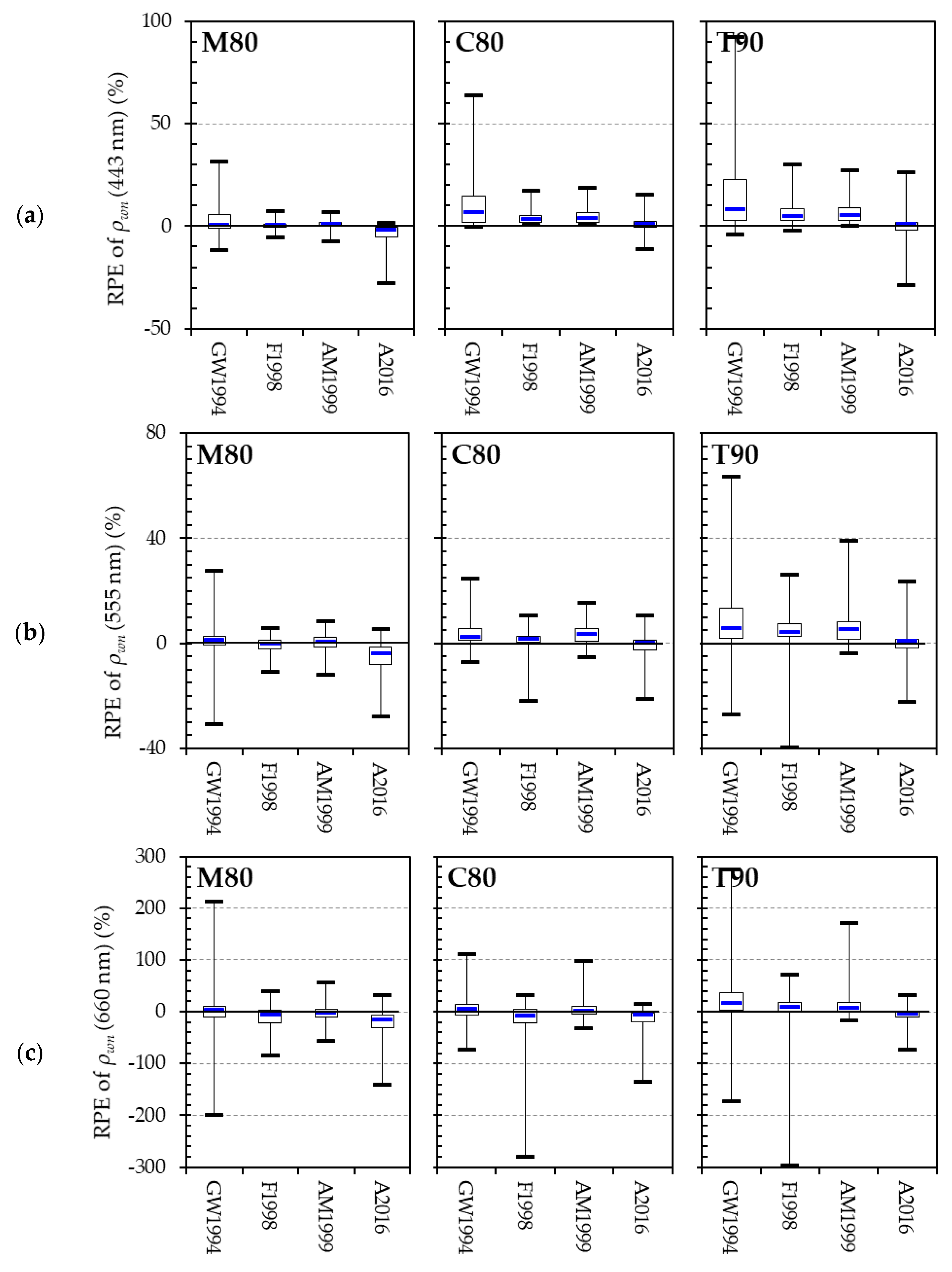
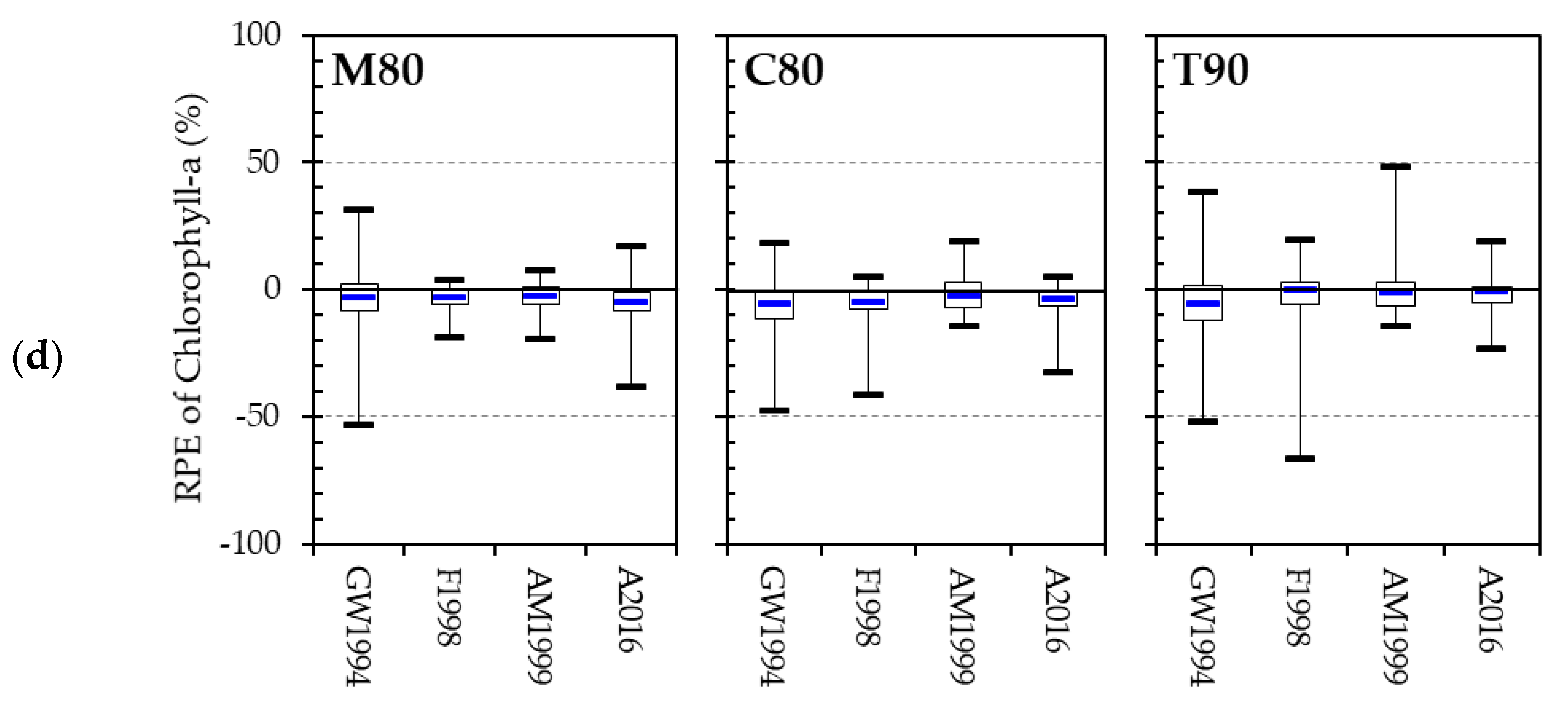
4. Results and Discussion

This section describes the atmospheric correction results and intermediate aerosol parameters over Case-1 waters for the three aerosol models specified, after integrating the four atmospheric correction schemes. For quantitative analysis of the four schemes, we used the following statistical parameters: error (Δ), relative percentage error (RPE), mean absolute percentage error (MAPE), median absolute percentage error (Med.), and root mean square error (RMSE), as follows:

$$\Delta =v_n^e-v_n^t$$

(31)

$$\mathrm{RPE}(\%)=100\left(\frac{\Delta }{v_n^t}\right)$$

(32)

$$\mathrm{MAPE}(\%)=\frac{1}{K}{\displaystyle \sum _{n=1}^K\left|\mathrm{RPE}\right|}$$

(33)

$$\mathrm{RMSE}=\sqrt{\frac{1}{n}{\displaystyle \sum _{n=1}^K\left({\Delta }^2\right)}}$$

(34)

where K is the total number of matched pairs, and v_n^t and v_n^e are the true and derived values of the nth matched entry, respectively.

The analysis was performed after replacing the four aerosol reflectance correction schemes within the atmospheric correction algorithm. The following nine aerosol models were used as candidates for the evaluation: oceanic model with RH 99% (O99), maritime model with RH 50, 70, 90, and 95% (M50, M70, M90, and M95, respectively), coastal model with RH 50 and 70% (C50 and C70, respectively), and tropospheric model with RH 50 and 80% (T50 and T80, respectively) [31]. We used the same radiative transfer code [22,23,24] for both the evaluation data and candidate aerosol look-up tables.

The results are summarized as box-and-whisker plots with median, minimum, maximum, and quartile values (Figure 1 and Figure 2). Figure 1a–c shows the errors (Δ) in aerosol reflectance retrieval at 443, 555, and 660 nm, respectively, for the four schemes. Figure 1d,e show the errors (Δ) in τ_a at 865 nm and the Ångström exponent for 443 nm relative to 865 nm, respectively. Figure 2a–c show the RPE in ρ_wn retrieval at 443, 555, and 660 nm, respectively.

Table 4. Statistical summary of atmospheric correction accuracy.

		ρwn(443 nm)			ρwn(555 nm)			ρwn(660 nm)
	Method	MAPE	Med.	RMSE	MAPE	Med.	RMSE	MAPE	Med.	RMSE
Total	GW1994	10.0%	5.1%	0.00198	6.7%	3.5%	0.00059	27.9%	14.4%	0.00032
	F1998	3.9%	2.4%	0.00068	3.5%	2.4%	0.00030	18.3%	12.5%	0.00023
	AM1999	4.3%	2.9%	0.00077	4.3%	3.3%	0.00035	11.9%	8.0%	0.00013
	A2016	3.4%	1.8%	0.00067	3.9%	2.2%	0.00034	15.6%	9.2%	0.00017
M80	GW1994	4.8%	2.4%	0.00098	4.5%	2.1%	0.00042	25.4%	10.9%	0.00031
	F1998	1.2%	0.9%	0.00021	2.0%	1.4%	0.00016	16.5%	11.5%	0.00016
	AM1999	1.8%	1.4%	0.00031	2.6%	2.0%	0.00021	11.2%	7.6%	0.00012
	A2016	4.1%	2.0%	0.00085	5.8%	4.0%	0.00045	22.0%	15.4%	0.00022
C80	GW1994	10.4%	6.4%	0.00187	4.5%	2.6%	0.00037	18.0%	11.5%	0.00019
	F1998	4.1%	3.2%	0.00062	2.5%	1.9%	0.00020	18.2%	11.7%	0.00023
	AM1999	4.9%	3.6%	0.00078	4.1%	3.6%	0.00029	10.5%	7.9%	0.00011
	A2016	2.7%	1.8%	0.00046	2.8%	1.6%	0.00024	14.5%	8.9%	0.00016
T90	GW1994	15.1%	8.2%	0.00275	11.1%	7.4%	0.00086	40.4%	22.3%	0.00042
	F1998	6.5%	4.8%	0.00099	6.1%	4.4%	0.00046	20.4%	13.8%	0.00028
	AM1999	6.5%	5.3%	0.00104	6.3%	5.0%	0.00048	14.1%	8.7%	0.00017
	A2016	3.4%	1.8%	0.00063	3.1%	1.6%	0.00027	9.9%	5.7%	0.00011

1.0% 40.0%, Color scale for mean absolute percentage error (MAPE).

summarizes the statistical results for ρ_wn retrieval, for the four schemes and three aerosol types. Note that A2016 uses Equation (10) for retrieval of the τ_a and Ångström exponent, because it does not calculate τ_a itself.

The median value of Δρ_am(443 nm) for the four schemes falls between −0.0011~+0.0007 (Figure 1). The GW1994, F1998, and AM1999 schemes tend to produce more errors, with underestimation of ρ_am retrieval for T90 aerosol models compared to the other models due to the underestimation of the aerosol optical thickness and Ångström exponent. In the A2016 scheme, on the contrary, ρ_am retrieval errors are more significant, with overestimation for M80 due to the overestimation of aerosol optical thickness and Ångström exponent.

The ρ_wn estimation results showed that the atmospheric correction accuracy for the four schemes was acceptable, with median APE values of ρ_wn of <5.1% and <3.5% at 443 nm and 555 nm, respectively. Although the RMSE of ρ_wn at 660 nm was smaller than that of ρ_wn at 443 nm, the MAPE of ρ_wn(660 nm) had a higher value than that of ρ_wn(443 nm), as the ρ_wn to aerosol reflectance ratio at 660 nm is significantly lower than that at 443 nm, due to relatively smaller water reflectance to aerosol reflectance ratio by relatively stronger water absorption at 660 nm. Similar to the aerosol estimation results, the accuracy of the ρ_wn estimation for the three schemes GW1994, F1998, and AM1999 improved for the coarse-sized aerosol models, in which aerosol reflectance had less of a multiple-scattering effect. The A2016 scheme showed relatively similar accuracy to the three aerosol models, in which the MAPE ranged from 2.7% to 4.1%.

5. Note and Summary

Two-NIR-band-based aerosol reflectance correction schemes have been widely employed. We implemented and tested four such aerosol correction schemes: SeaWiFS/MODIS/VIIRS (GW1994), OCTS/GLI/SGLI (F1998), MERIS/OLCI (AM1999), and GOCI/GOCI-II (A2016). The GW1994 scheme determines the contribution of the aerosol models in the single-scattering domain after conversion from aerosol multiple- to single-scattering reflectance. F1998 determines the contribution to the aerosol optical thickness domain and then uses a weighted average approach to enhance the calculation accuracy of the weighting factors, whereas GW1994 uses an average value. AM1999 determines the contribution in the multiple-scattering domain and then uses linear distance to calculate the weighting factor. There are methods [28,34] that apply an approach similar to that of AM1999 to determine the contribution based on the linear distance of the reflectance in the multiple-scattering domain; these methods are expected to offer comparable performance to that of AM1999. A2016 is similar to AM1999 in terms of selecting aerosol models in the multiple-scattering domain, except that the weighting scheme for A2016 is enhanced to consider the wavelength-dependent weighting factor.

In this study, we intercompared four aerosol correction schemes in an assimilation. However, discrepancies between aerosol models and the actual aerosols can introduce more significant errors than the inaccuracies associated with the inverse scheme. Two-NIR aerosol correction schemes that we evaluated rely on the assumption of non- or less-absorbent aerosol optical properties, although actual aerosols originating from land can absorb more light. Alternative aerosol models are being developed that provide a more realistic representation of the optical properties of aerosols [35]; however, these models are also based on non- or less-absorbent models. All these schemes will significantly underestimate the ρ_wn for strongly absorbing aerosols that contain a soot component, as discussed by the IOCCG study [21]. To determine absorbance properties future aerosol correction schemes will require additional aerosol information from other wavelengths, i.e., from the near-ultraviolet regime [17] or from polarization [36]. Errors in variables such as wind speed [37], trace gases [38,39,40,41], and air pressure [38] are higher at higher solar and sensor zenith angles. The atmospheric correction accuracy is also impacted by the system vicarious calibration [42,43,44]. The radiance calibration requirement for atmospheric correction is <1%. However, the visible calibration gain can be varied by more than 1% due to different NIR intercalibration. Further work on the NIR calibration is needed to improve this.

The most recent atmospheric correction algorithms yield errors of less than 5% [2,45], which satisfies the accuracy requirement for ocean colour observations in the open ocean. However, more accurate atmospheric correction algorithms are required to observe diurnal changes from geostationary platforms such as GOCI, since geostationary measurements are made over a wide range of solar zenith angles which significantly increases the atmospheric correction uncertainty. Therefore, further investigation on the error sources from all relevant parameters is needed to improve atmospheric correction algorithms.

References

1. McClain, C.R.; Feldman, G.C.; Hooker, S.B. An overview of the SeaWiFS project and strategies for producing a climate research quality global ocean bio-optical time series. Deep Sea Res. Part II Top. Stud. Oceanogr. 2004, 51, 5–42. [Google Scholar] [CrossRef]
2. Esaias, W.E.; Abbott, M.R.; Barton, I.; Brown, O.B.; Campbell, J.W.; Carder, K.L.; Clark, D.K.; Evans, R.H.; Hoge, F.E.; Gordon, H.R.; et al. An overview of MODIS capabilities for ocean science observations. IEEE Trans. Geosci. Remote Sens. 1998, 36, 1250–1265. [Google Scholar] [CrossRef] [Green Version]
3. Kawamura, H.; OCTS Team. OCTS mission overview. J. Oceanogr. 1998, 54, 383–399. [Google Scholar] [CrossRef]
4. Rast, M.; Bezy, J.L.; Bruzzi, S. The ESA Medium Resolution Imaging Spectrometer MERIS a review of the instrument and its mission. Int. J. Remote Sens. 1999, 20, 1681–1702. [Google Scholar] [CrossRef]
5. Tanaka, K.; Kurihara, S.; Okamura, Y. The sensor characterization of global imager (GLI) on ADEOS-II satellite. IEICE Trans. Commun. 2005, J88-B, 151–157. [Google Scholar]
6. Tanaka, K.; Okamura, Y.; Amano, T.; Hiramatsu, M.; Shiratama, K. Operation concept of the second-generation global imager (SGLI). In Earth Observing Missions and Sensors: Development, Implementation, and Characterization. Int. Soc. Opt. Photonics 2010, 7862, 786209. [Google Scholar]
7. Kang, G.; Coste, P.; Youn, H.; Faure, F.; Choi, S. An in-orbit radiometric calibration method of the geostationary ocean color imager. IEEE Trans. Geosci. Remote Sens. 2010, 48, 4322–4328. [Google Scholar] [CrossRef]
8. Wang, M.; Liu, X.; Jiang, L.; Son, S.; Sun, J.; Shi, W.; Tan, L.; Naik, P.; Mikelsons, K.; Wang, X.; et al. Evaluation of VIIRS ocean color products. In Ocean Remote Sensing and Monitoring from Space. Int. Soc. Opt. Photonics 2014, 9261, 92610E. [Google Scholar]
9. Gordon, H.R.; Wang, M. Retrieval of water-leaving radiance and aerosol optical thickness over the oceans with SeaWiFS: A preliminary algorithm. Appl. Opt. 1994, 33, 443–452. [Google Scholar] [CrossRef] [PubMed]
10. Wang, M.; Gordon, H.R. A simple, moderately accurate, atmospheric correction algorithm for SeaWiFS. Remote Sens. Eviron. 1994, 50, 231–239. [Google Scholar] [CrossRef]
11. Gordon, H.R.; Brown, J.W.; Evans, R.H. Exact Rayleigh scattering calculations for use with the Nimbus-7 coastal zone color scanner. Appl. Opt. 1988, 27, 862–871. [Google Scholar] [CrossRef] [PubMed]
12. Gordon, H.R.; Wang, M. Surface-roughness considerations for atmospheric correction of ocean color sensors. 1: The Rayleigh-scattering component. Appl. Opt. 1992, 31, 4247–4260. [Google Scholar] [CrossRef] [PubMed]
13. Wang, M. The Rayleigh lookup tables for the SeaWiFS data processing: Accounting for the effects of ocean surface roughness. Int. J. Remote Sens. 2002, 23, 2693–2702. [Google Scholar] [CrossRef]
14. Wang, M. A refinement for the Rayleigh radiance computation with variation of the atmospheric pressure. Int. J. Remote Sens. 2005, 26, 5651–5663. [Google Scholar] [CrossRef]
15. Wang, M. Rayleigh radiance computations for satellite remote sensing: Accounting for the effect of sensor spectral response function. Opt. Express 2016, 24, 12414–12429. [Google Scholar] [CrossRef] [PubMed]
16. Fukushima, H.; Higurashi, A.; Mitomi, Y.; Nakajima, T.; Noguchi, T.; Tanaka, T.; Toratani, M. Correction of atmospheric effect on ADEOS/OCTS ocean color data: Algorithm description and evaluation of its performance. J. Oceanogr. 1998, 54, 417–430. [Google Scholar] [CrossRef]
17. Toratani, M.; Fukushima, H.; Murakami, H.; Tanaka, A. Atmospheric correction scheme for GLI with absorptive aerosol correction. J. Oceanogr. 2007, 63, 525–532. [Google Scholar] [CrossRef]
18. Antoine, D.; Morel, A. A multiple scattering algorithm for atmospheric correction of remotely sensed ocean colour (MERIS instrument): Principle and implementation for atmospheres carrying various aerosols including absorbing ones. Int. J. Remote Sens. 1999, 20, 1875–1916. [Google Scholar] [CrossRef]
19. Antoine, D. Atmospheric Corrections over Case 1 Waters (CWAC) OLCI Level 2 ATBD 2010, v.2.2. S3-L2-SD-03-C07-LOV-ATBD. Available online: https://earth.esa.int/documents/247904/349589/OLCI_L2_ATBD_Atmospheric_Corrections_case-1_waters.pdf (accessed on 31 October 2016).
20. Ahn, J.H.; Park, Y.J.; Kim, W.; Lee, B. Simple aerosol correction technique based on the spectral relationships of the aerosol multiple-scattering reflectances for atmospheric correction over the oceans. Opt. Express 2016, 24, 29659–29669. [Google Scholar] [CrossRef] [PubMed]
21. IOCCG. Atmospheric correction for remotely-sensed ocean-colour products. In Reports of International Ocean-Colour Coordinating Group 2010; Wang, M., Ed.; IOCCG: Dartmouth, NS, Canada, 2010. [Google Scholar]
22. Vermote, E.F.; Tanré, D.; Deuze, J.L.; Herman, M.; Morcette, J.J. Second simulation of the satellite signal in the solar spectrum, 6S: An overview. IEEE Trans. Geosci. Remote Sens. 1997, 35, 675–686. [Google Scholar] [CrossRef]
23. Kotchenova, S.Y.; Vermote, E.F.; Matarrese, R.; Klemm, F.J., Jr. Validation of a vector version of the 6S radiative transfer code for atmospheric correction of satellite data. Part I: Path radiance. Appl. Opt. 2006, 45, 6762–6774. [Google Scholar] [CrossRef] [PubMed]
24. Kotchenova, S.Y.; Vermote, E.F. Validation of a vector version of the 6S radiative transfer code for atmospheric correction of satellite data. Part II. Homogeneous Lambertian and anisotropic surfaces. Appl. Opt. 2007, 46, 4455–4464. [Google Scholar] [CrossRef] [PubMed]
25. Franz, B. rhoa_to_rhoas()—MS Aerosol Reflectance to SS Aerosol Reflectance, aerosol.c in SeaDAS Code 2004. Available online: http://seadas.gsfc.nasa.gov (accessed on 31 October 2016).
26. Wang, M. Correction of artifacts in the SeaWiFS atmospheric correction: Removing discontinuity in the derived products. Remote Sens. Environ. 2003, 84, 603–611. [Google Scholar] [CrossRef]
27. Ahmad, Z.; Franz, B. Atmospheric correction using multiple-scattering epsilon values. In Proceedings of the Ocean Optics XXII, Portland, MA, USA, 26–31 October 2014. [Google Scholar]
28. Antoine, D.; Morel, A. Relative importance of multiple scattering by air molecules and aerosols in forming the atmospheric path radiance in the visible and near-infrared parts of the spectrum. Appl. Opt. 1998, 37, 2245–2259. [Google Scholar] [CrossRef] [PubMed]
29. Morel, A.; Maritorena, S. Bio-optical properties of oceanic waters: A reappraisal. J. Geophys. Res. 2001, 106, 7163–7180. [Google Scholar] [CrossRef] [Green Version]
30. Siegel, D.A.; Wang, M.; Maritorena, S.; Robinson, W. Atmospheric correction of satellite ocean color imagery: The black pixel assumption. Appl. Opt. 2000, 39, 3582–3591. [Google Scholar] [CrossRef] [PubMed]
31. Shettle, E.P.; Fenn, R.W. Models for the Aerosols of the Lower Atmosphere and the Effects of Humidity Variations on Their Optical Properties. Air Force Geophysics Lab Hanscom Afb Ma. 1979, No. AFGL-TR-79-0214. Available online: http://www.dtic.mil/docs/citations/ADA085951 (accessed on 17 September 2018).
32. SeaWiFS Reprocessing #4 (2002)—Case 7: Improved Cloud Flagging Method. Available online: https://oceancolor.gsfc.nasa.gov/reprocessing/r2002/seawifs/ (accessed on 10 June 2018).
33. O’Reilly, J.E.; Maritorena, S.; Mitchell, B.G.; Siegel, D.A.; Carder, K.L.; Garver, S.A.; Kahru, M.; McClain, C. Ocean color chlorophyll algorithms for SeaWiFS. J. Geophys. Res. 1998, 103, 24937–24953. [Google Scholar] [CrossRef] [Green Version]
34. Wang, M. Extrapolation of the aerosol reflectance from the near-infrared to the visible: The single-scattering epsilon vs multiple-scattering epsilon method. Int. J. Remote Sens. 2004, 25, 3637–3650. [Google Scholar] [CrossRef]
35. Ahmad, Z.; Franz, B.A.; McClain, C.R.; Kwiatkowska, E.J.; Werdell, J.; Shettle, E.P.; Holben, B.N. New aerosol models for the retrieval of aerosol optical thickness and normalized water-leaving radiance from the SeaWiFS and MODIS sensors over coastal regions and open oceans. Appl. Opt. 2010, 49, 5545–5560. [Google Scholar] [CrossRef] [PubMed]
36. Chowdhary, J.; Tsigaridis, K.; Nelson, N. Spaceborne ocean color remote sensing in the UV-A part of the spectrum. In Proceedings of the Ocean Optics XXIV, Dubrovnik, Croatia, 7–12 October 2018. [Google Scholar]
37. Gordon, H.R.; Wang, M. Surface-roughness considerations for atmospheric correction of ocean color sensor. 2: Error in the retrieved water-leaving radiance. Appl. Opt. 1992, 31, 4261–4267. [Google Scholar] [CrossRef] [PubMed]
38. André, J.M.; Morel, A. Simulated effects of barometric pressure and ozone content upon the estimate of marine phytoplankton from space. J. Geophys. Res. 1989, 94, 1029–1037. [Google Scholar] [CrossRef]
39. Tzortziou, M.; Herman, J.R.; Ahmad, Z.; Loughner, C.P.; Abuhassan, N.; Cede, A. Atmospheric NO2 dynamics and impact on ocean color retrievals in urban nearshore regions. J. Geophys. Res. 2014, 119, 3834–3854. [Google Scholar] [CrossRef]
40. Tzortziou, M.; Parker, O.; Lamb, B.; Herman, J.; Lamsal, L.; Stauffer, R.; Abuhassan, N. Atmospheric Trace Gas (NO2 and O3) Variability in South Korean Coastal Waters, and Implications for Remote Sensing of Coastal Ocean Color Dynamics. Remote Sens. 2018, 10, 1587. [Google Scholar] [CrossRef]
41. Pahlevan, N.; Ahn, J.H. Uncertainty in atmospheric parameters for diurnal remote sensing of coastal oceans. In Proceedings of the Ocean Optics XXIV, Dubrovnik, Croatia, 7–12 October 2018. [Google Scholar]
42. Wang, M.; Gordon, H.R. Calibration of ocean color scanners: How much error is acceptable in the near infrared? Remote Sens. Eviron. 2002, 82, 497–504. [Google Scholar] [CrossRef]
43. Franz, B.A.; Bailey, S.W.; Werdell, P.J.; Morel, A.; McClain, C.R. Sensor-independent approach to the vicarious calibration of satellite ocean color radiometry. Appl. Opt. 2007, 46, 5068–5082. [Google Scholar] [CrossRef] [PubMed]
44. Pahlevan, N.; Roger, J.C.; Ahmad, Z. Revisiting short-wave-infrared (SWIR) bands for atmospheric correction in coastal waters. Opt. Express 2017, 25, 6015–6035. [Google Scholar] [CrossRef] [PubMed]
45. Wang, M.; Gordon, H.R. Sensor performance requirements for atmospheric correction of satellite ocean color remote sensing. Opt. Express 2018, 26, 7390–7403. [Google Scholar] [CrossRef] [PubMed]
Figure 1. Errors in aerosol retrieval for the four schemes, presented as box-and-whisker plots. Aerosol reflectance differences by scheme for (a) the blue band (443 nm); (b) the green band (555 nm); and (c) the red band (660 nm); (d) aerosol optical thickness difference by scheme for the green band; and (e) aerosol Ångström exponent for 443 nm relative to 865 nm.
Remotesensing 10 01791 g001aRemotesensing 10 01791 g001b
Figure 2. Water reflectance (ρwn) retrieval accuracy of the (a) blue; (b) green; and (c) red bands in the atmospheric correction algorithm after integrating the four aerosol correction schemes. Chlorophyll-a estimation error based on OC3 [33] is plotted in (d).
Remotesensing 10 01791 g002aRemotesensing 10 01791 g002b