Article

Relating Spatiotemporal Patterns of Forest Fires Burned Area and Duration to Diurnal Land Surface Temperature Anomalies

by
Carmine Maffei
1,2,*,
Silvia Maria Alfieri
1 and
Massimo Menenti
1
1
Department of Geoscience and Remote Sensing, Delft University of Technology, Stevinweg 1, 2628CN Delft, The Netherlands
2
Leicester Innovation Hub, University of Leicester, University Road, Leicester LE1 7RH, UK
*
Author to whom correspondence should be addressed.
Remote Sens. 2018, 10(11), 1777; https://doi.org/10.3390/rs10111777
Submission received: 8 October 2018 / Revised: 2 November 2018 / Accepted: 7 November 2018 / Published: 9 November 2018
(This article belongs to the Special Issue Multitemporal Remote Sensing for Forestry)

Abstract

:
Forest fires are a major source of ecosystem disturbance. Vegetation reacts to meteorological factors contributing to fire danger by reducing stomatal conductance, thus leading to an increase of canopy temperature. The latter can be detected by remote sensing measurements in the thermal infrared as a deviation of observed land surface temperature (LST) from climatological values, that is as an LST anomaly. A relationship is thus expected between LST anomalies and forest fires burned area and duration. These two characteristics are indeed controlled by a large variety of both static and dynamic factors related to topography, land cover, climate, weather (including those affecting LST) and anthropic activity. To investigate the predicting capability of remote sensing measurements, rather than constructing a comprehensive model, it would be relevant to determine whether anomalies of LST affect the probability distributions of burned area and fire duration. This research approached the outlined knowledge gap through the analysis of a dataset of forest fires in Campania (Italy) covering years 2003–2011 against estimates of LST anomaly. An LST climatology was first computed from time series of daily Aqua-MODIS LST data (product MYD11A1, collection 6) over the longest available sequence of complete annual datasets (2003–2017), through the Harmonic Analysis of Time Series (HANTS) algorithm. HANTS was also used to create individual annual models of LST data, to minimize the effect of varying observation geometry and cloud contamination on LST estimates while retaining its seasonal variation. LST anomalies where thus quantified as the difference between LST annual models and LST climatology. Fire data were intersected with LST anomaly maps to associate each fire with the LST anomaly value observed at its position on the day previous to the event. Further to this step, the closest probability distribution function describing burned area and fire duration were identified against a selection of parametric models through the maximization of the Anderson-Darling goodness-of-fit. Parameters of the identified distributions conditional to LST anomaly where then determined along their confidence intervals. Results show that in the study area log-transformed burned area is described by a normal distribution, whereas log-transformed fire duration is closer to a generalized extreme value (GEV) distribution. The parameters of these distributions conditional to LST anomaly show clear trends with increasing LST anomaly; significance of this observation was verified through a likelihood ratio test. This confirmed that LST anomaly is a covariate of both burned area and fire duration. As a consequence, it was observed that conditional probabilities of extreme events appear to increase with increasing positive deviations of LST from its climatology values. This confirms the stated hypothesis that LST anomalies affect forest fires burned area and duration and highlights the informative content of time series of LST with respect to fire danger.

Graphical Abstract

1. Introduction

Forest fires are a source of significant ecosystem damage at global scale, as they affect the biogeochemical cycle, are a source of atmospheric emissions, alter the net carbon balance, disturb forest structure and cause long-term changes in soil properties [1,2,3,4,5]. Fires also condition anthropic activities as they threaten human lives, have a negative effect on quality of life and cause economic losses [6,7,8]. Increasing concern derives from the observation that climate change is negatively affecting spatial and temporal patterns of fire disturbance [9,10,11,12].
In Mediterranean ecosystems, prolonged droughts and heat waves create the preconditions for increases in frequency and intensity of forest fires [13,14], the underlying mechanism being the reduction of live and dead fuels moisture content as a response of the soil-plant system to increased vapor-pressure deficit [11,15,16]. Vegetation response varies with species as well as with forest structure and soil/terrain characteristics and it is determined by evapotranspiration [17,18,19]. The moisture of dead fuels, which include the organic elements of forest litter such as senescent grasses, dry leaves, small twigs and compacted organic material in the topsoil, is affected by weather variations as well and it is regulated through evaporation [20,21,22]. The moisture content of both alive and dead fuels are thus affected by weather forcing and indeed vegetation stress status has been found to be related to some meteorological drought indexes, which in turn are related to moisture content of the largest size classes of dead fuels [14,23,24,25,26,27].
The vegetation transpiration regulation mechanism reacts to water stress conditions by reducing stomatal conductance, thus leading to an increase of canopy temperature [28,29,30]. This phenomenon can be detected by satellite measurements in the thermal infrared and has been widely used in the development of methodologies based on the satellite retrieval of land surface temperature (LST) to map vegetation stress conditions [31,32,33,34,35]. As moisture content has a direct relationship with live fuels ignitability and flames propagation [36,37,38,39], a relationship between LST and forest fires may be expected [40,41,42]. Indeed, several approaches use LST in association with optical spectral indexes of vegetation greenness or moisture content to construct physically based or empirical fire danger rating systems [43,44,45,46,47,48]. Some researchers used LST to model energy budgets [40,49,50] or to estimate heat energy of pre-ignition [51] and predict fire occurrence.
Little research was conducted to relate LST to fire characteristics. Post-fire LST was used to quantify burnt severity either alone [52,53,54] or in conjunction with optical data [55,56]. Pre-event LST was used, along with other factors, to model burned area but results were ambiguous [57]. While evidence supports the hypothesis that higher surface temperature is associated with an increased fire occurrence [58,59,60], no such relationship was previously investigated against burned area or fire duration.
Burned area is indeed controlled by a large variety of both static and dynamic factors, essentially falling into five groups: topography, such as elevation, slope, south-westness (in the northern hemisphere) or north-westness (in the southern hemisphere); land cover, including vegetation type, composition, connectivity, fuel load, pyrodiversity; climate, for example annual average daily maximum and minimum temperature; weather (including active drivers of fuel moisture) such as cumulative antecedent precipitation, wind speed, relative humidity; anthropic activity, including land development, road density, distance to settlements, fire prevention and contrasting strategies [61,62,63,64,65,66,67]. While less studied, fire duration appears to be related to similar factors [68,69,70,71]. Among these factors, only those affecting vegetation moisture are actually related to LST. To investigate the predicting capability of remote sensing measurements, rather than constructing a comprehensive model, it would be relevant to determine whether an increase in LST affects the probability distributions of burned area and fire duration. Since an increase of LST would be evaluated against an LST climatology, thus implicitly implying the evaluation of a delta or anomaly, the objective would in other terms be to assess if such an anomaly is a covariate of the two named fire characteristics.
The research described in this document follows from this line of reasoning and tried to verify if a relationship linking anomalies of LST to burned area and fire duration exists, thus exploring the identified knowledge gap. The analyses were performed on the study area of Campania, Italy, for which a dataset comprising more than 8800 fire events recorded between 2003 and 2011 was made available by local authorities.
The accomplishment of the stated objective first required the definition of a method for the quantification of LST anomalies. Crucial to this step was the prior modelling of an LST climatology. Indeed, multitemporal analysis was suggested as a mean to determine seasonal minima against which to assess LST values triggering fire occurrence [58,72,73,74]. To this purpose, the longest available time series of daily Aqua-MODIS LST data was processed with the Harmonic Analysis of Time Series (HANTS) algorithm [75,76] to construct a daily pixel-wise climatology of LST. HANTS was also used to process annual time series of LST and create cloud- and noise-free annual models of daily LST. LST anomalies were finally evaluated as the difference between the LST annual models and the LST climatology.
Further steps required the analysis of the fire data towards the identification of the closest fitting probability density function describing burned area and fire duration. The fire database was then intersected with daily maps of LST anomalies and each fire was associated with the corresponding LST anomaly value occurring at the same location on the day previous to the event. Parameters of the identified distributions conditional to LST anomaly values were determined along their confidence intervals and trends were identified [77]. Finally, probability of extreme events conditional to LST anomaly were evaluated.

2. Materials and Methods
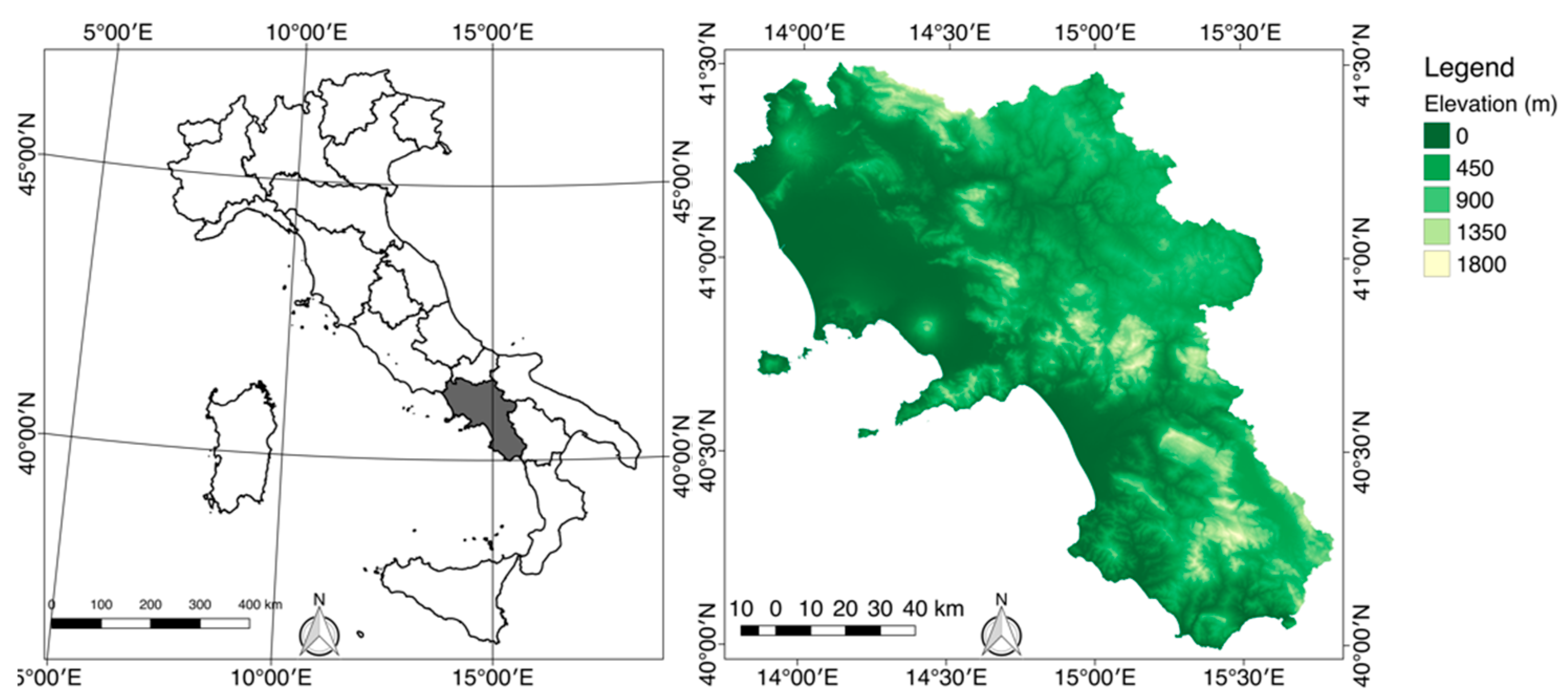
2.1. Study Area

The research focused on Campania, Italy (40°83′N, 14°13′E, 13,595 km2, Figure 1). The interest in this region is given by its position in the middle of the Mediterranean and by the diversity of its landscape. The land cover is characterized by agricultural areas prevailing in plains and semi-natural forest-dominated areas covering hills and mountains [78]. Campania is among the most densely populated regions of Mediterranean Europe, almost all fires are triggered by human activities and fire incidence is considered high [79,80].

2.2. Data

2.2.1. MODIS LST Data

A dataset of daily gridded Aqua-MODIS LST data (product MYD11A1, collection 6) from 2003 to 2017 retrieved from the Land Processes Distributed Active Archive Centre (LP DAAC, https://e4ftl01.cr.usgs.gov/) was used for this research. MYD11 products are generated by an angle-dependent split-window algorithm exploiting the differential atmospheric absorption in MODIS bands 31 (11 µm) and 32 (12 µm) to determine LST values from radiance measurements of clear-sky pixels. The achieved mean LST error is typically within ±0.6 K and the standard deviation of validation errors is typically less than 0.5 K [81].
Product MYD11A1 contains both diurnal (13:30) and nocturnal (1:30) LST measurements, along with corresponding quality assurance information. Preference was given to diurnal rather than nocturnal data and to Aqua-MODIS rather than Terra-MODIS, to capture canopy temperature variations due to water stress occurring at the hour of the day when maximum air temperature is approximatively achieved. Retrieved LST estimates were further masked against MYD11A1 pixel-wise quality assurance (QA) metadata and only data marked as good quality (QA bits 1,0 = 00), that is retrieved at nominal radiometric and clear-sky conditions, were retained [82,83]. However, this approach does not ensure that all cloud contaminated pixels are excluded from further processing [84].

2.2.2. Fire Data

A dataset of about 8800 fires officially recorded in Campania between 2003 and 2011 was provided by the Natural Resources Unit of Carabinieri, a law enforcement agency in charge of forest fires prevention, firefighting, arson investigations and prosecution and burned area inventorying. The database details the presumed date and time of fire ignition, recorded date and time of fire extinction, geographic coordinates of burned area centroid, total burned area and presumed causes. While Carabinieri actually record burnt scar perimeters on a fire-by-fire basis, according to conventional practices of field surveying with GPS receivers and desk digital cartography, these were not provided for this research. However, for the purpose of this study, this is not a source of concern on the positional accuracy of the provided centroids, as only 53 fires (0.87% of the fires in the dataset) are larger than 1 km2, that is of a MODIS pixel in the thermal bands.
The dataset covered a range of fire seasons that were considered safe to critical in both number of fires and total burnt area. Most fires (84%) occur in the summer season, that is June to September. About 99.8% of fires are of human origin (negligent or arson). On average, 980 fires are recorded each year, leading to the loss of more than 6160 hectares of natural areas, including 4190 ha of forests.
Fires in the database were overlaid on the CORINE Land Cover (CLC) map [85] to select those occurred in vegetated and recently burned areas only. CLC maps are produced at a nominal scale of 1:100.000, with a minimum mapping unit of 25 ha and minimum width of linear elements of 100 m and are updated every six years. Fires occurred between 2003 and 2008 were intersected with CLC 2006, while fires between 2009 and 2011 were intersected with CLC 2012. A total of more than 6100 events occurred in land cover classes reported in Table 1 were used in this research, thus excluding events recorded on agricultural land.
Observed burned area encompasses five orders of magnitude, while its average is 7.1 ha. The 95th percentile of burned area is 27.8 ha; this quantity was used as a reference for extreme events in the region. Analogously, mean fire duration is 9.4 h and the 95th percentile is 27.5 h.

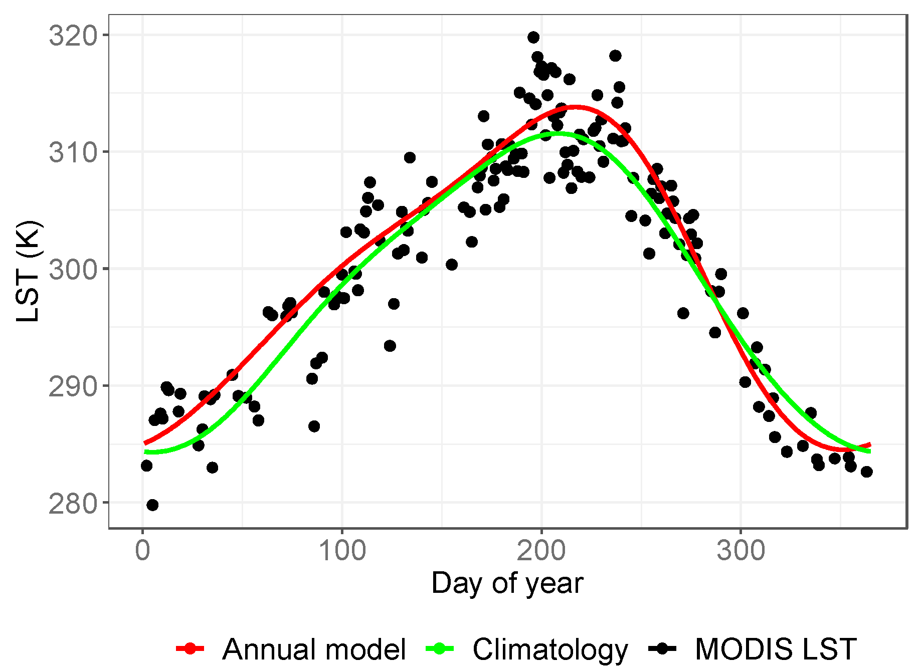
2.3. Modelling Temporal Patterns of LST

The modelling of the LST climatology and of LST annual models was performed by means of the Harmonic Analysis of Time Series (HANTS) algorithm [75,76]. This method was initially proposed to fill in missing or cloudy observations and to remove outliers in time series of NDVI data by exploiting its periodic behaviour [86,87] and later used also with LST series, for example [83,88,89].
A temporal sequence of N images I(x, y, ti), i = 1, 2, …, N, can be described as a Fourier series:
I ( x , y , t i ) = a 0 ( x , y ) + j = 1 M a j ( x , y ) × cos ( ω j t i φ j ( x , y ) )
where I(x, y, ti) is the LST retrieved from MODIS measurements at pixel longitude x, pixel latitude y, day ti when the ith image was taken, ωj is the frequency of the jth harmonic term in the Fourier series, M is the number of frequencies of the Fourier series, aj(x, y) and ϕj(x, y) are the amplitude and the phase of the jth harmonic term. The harmonic frequencies are integer multiples of the base frequency, that is,
ω j = ( 2 π / L ) × j
where L is the length of the base period. Because the zero frequency has no phase, the amplitude related to the zero frequency a0(x, y) is equal to the average of all N observations of I(x, y, ti) [89].
HANTS handles the Fourier analysis as a least squares curve fitting problem within an iterative approach. In the first step, the least squares curve fitting is performed using all valid data in the series. In the second step, observations that deviate from the curve determined in the first iteration more than a pre-defined threshold (the fit error tolerance, FET) in the specified direction of rejection (lower values or higher values) are removed and the remaining data are used to compute the least square curve fitting again. The iterations are repeated until either all the remaining observations are within the FET or the number of remaining data points becomes less than the specified degree of over determinedness (DOD) [90].

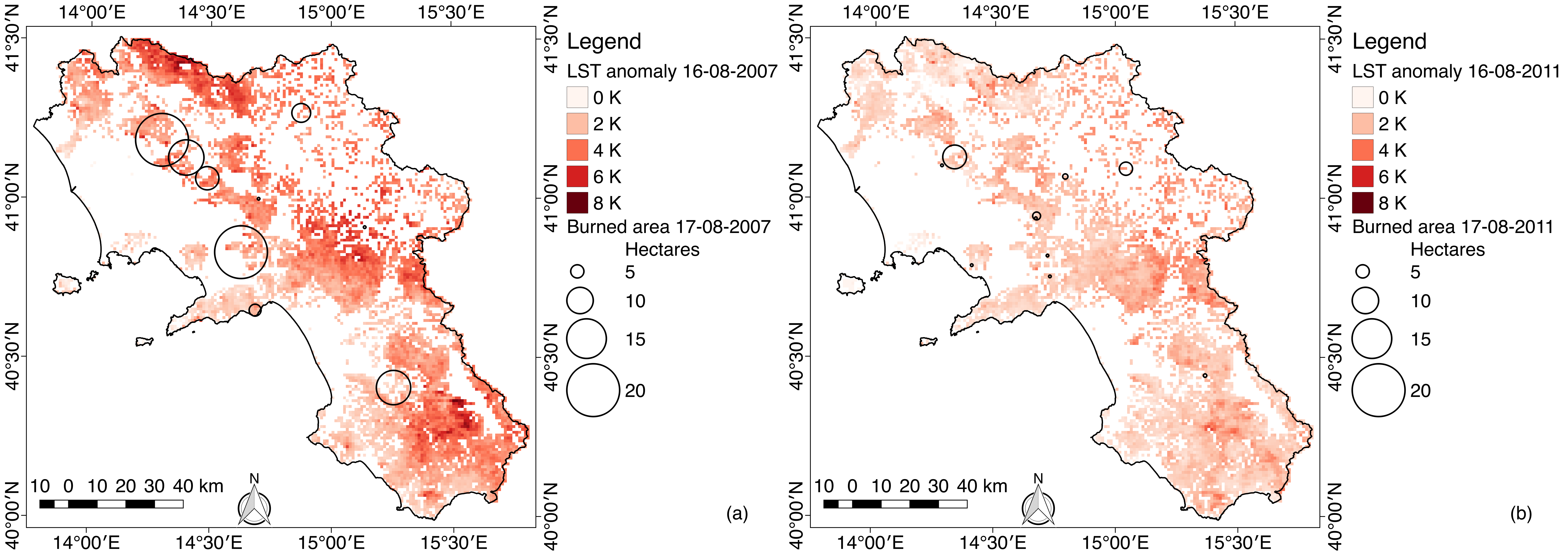
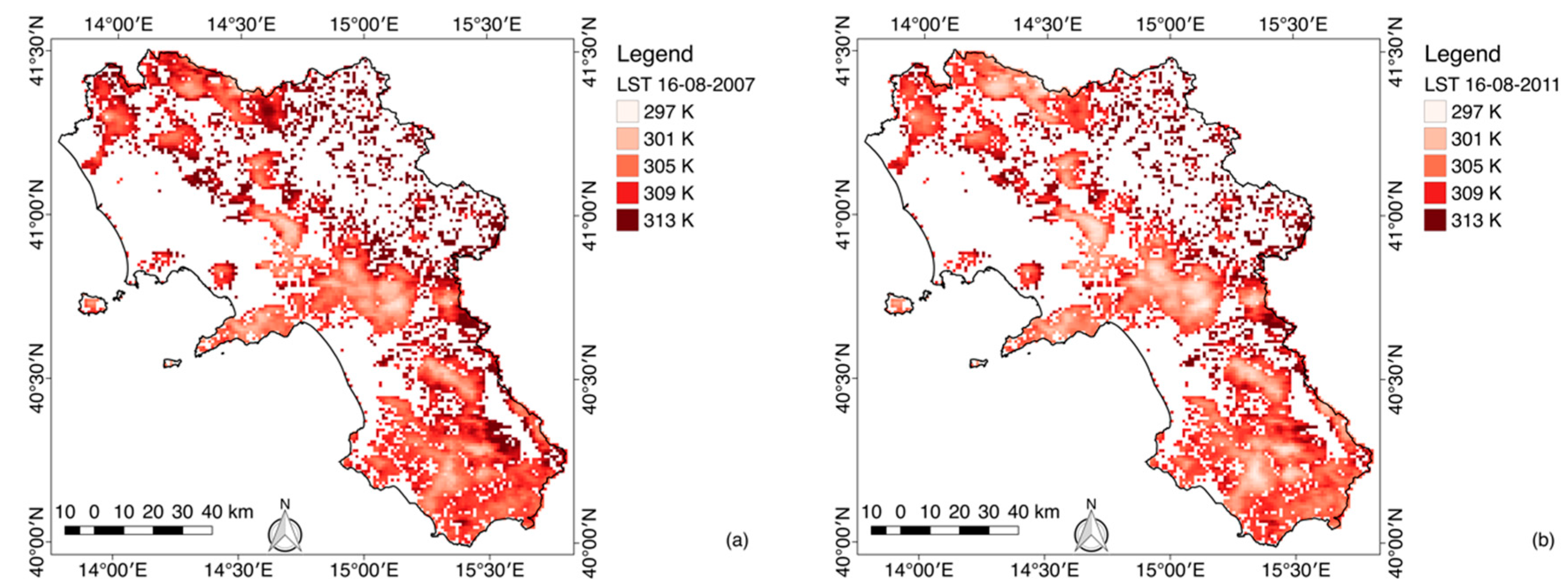
2.4. Evaluation of Land Surface Temperature Anomaly

HANTS was used to decompose the time series of MODIS LST retrievals into their descriptive significant periodic components. Series comprising the first three harmonics were fit to the data with two different methods:
  • HANTS was executed on yearly sequences 2003–2011 of daily LST data individually to construct annual models of daily LST [82]. The objective of this approach was the removal of LST variability due to undetected cloud contamination and varying observation geometry while modelling LST annual variation. The result was a collection of new annual series of daily LST maps, one for each year being considered, computed from the identified harmonic components. These were used as representative of actual measurements.
  • The algorithm was executed on the whole 2003–2017 data set, with a base period of one year, to construct a pixel-wise daily climatology of LST [88]. The need of using this climatology as a basis for the calculation of thermal anomalies suggested its evaluation from the longest available sequence of complete annual datasets of daily MODIS LST data. The output of this process is a new series of daily LST maps computed from the identified harmonic components, representative of daily climatological values of LST.
A synthesis of the HANTS parameters adopted in the two approaches is reported in Table 2. In both, the base period is one year and the number of frequencies is set to three. The direction of outliers rejection was set as “Lo”, thus leading to the removal of all data points that are more than FET lower than the fitted harmonics, according to the fact that cloud contamination in pixels causes an underestimation of LST. The development of the LST climatology is based on a more relaxed FET value, as opposed to annual models, to compensate for its inter-annual variability. The degree of over determinedness was dynamically adjusted on a per-pixel basis as the half of LST estimates marked as good quality in the QA of MYD11A1 product.
Figure 2 depicts one year of clear-sky Aqua-MODIS LST retrievals in a sample pixel within the study area, along with the corresponding LST annual model and the LST climatology. It can be observed that the annual model captures LST variation throughout the year, while filtering its variability. LST climatology, derived from the 2003–2017 series of daily LST data, shows a distinct pattern. In this example, the annual model of LST is higher than the LST climatology for most of the year.
A land surface temperature anomaly is hereby defined as the difference between LST annual models and the LST climatology. At a given day ti the anomaly is positive when the LST annual model is higher that the LST climatology. In this sense, LST anomalies quantify the deviation of LST from the climatology value expected in that pixel (Figure 2). The approach of using the LST annual model rather than the actual measurements of LST hinders the detection of LST variations occurring over a short period of time. Nevertheless, it quantifies the build-up of the LST anomaly throughout the dry season while filtering the variability in LST estimates due to observation geometry, residual cloud contamination and retrieval accuracy. This in turns allows the appreciation of LST anomalies with values below the accuracies provided by the MYD11A1 algorithm and provides measurements in dates when complete cloud cover is present [88].
Daily maps of LST anomaly were produced for the entire observation period between 2003 and 2011. These maps were intersected with fire data, so that each fire was associated with the value of the LST anomaly in the same location on the day previous to the event.

2.5. Parametric Distributions of Burned Area and Fire Duration

Burned area and fire duration relate to the difficulty of control of fires and to the damage they cause and thus to fire danger [91,92]. Prior to any investigation on the relationship between these fire characteristics and LST anomalies, their probability distributions were identified.
Several parametric distributions are reported in literature to fit burned area, including normal [93], log-normal [94,95], exponential [93,96,97], gamma [97], generalized extreme value [98] and Weibull [99]. A limited number of papers report on parametric distributions of fire duration for example [100]. The diversity of these results highlights that no one single model can be identified to describe fire size distribution globally, due to the diversity of encompassed terrain, climate, ecology, forest and fire management practices [99,101] and that the closest fitting model needs to be identified on a regional basis.
In this study, both fire size and fire duration datasets were tested against the following parametric models:
  • Normal
    f ( x | μ , σ ) = 1 2 π σ exp [ ( x μ ) 2 2 σ 2 ]
  • Log-normal
    f ( x | μ , σ ) = 1 2 π σ x exp [ ( ln x μ ) 2 2 σ 2 ]
  • Exponential
    f ( x | λ ) = λ exp ( λ x )
  • Gamma
    f ( x | a , s ) = 1 s a Γ ( a ) x a 1 exp ( x / s )
  • Generalized extreme value (GEV)
    f ( x | a , b , s ) = 1 b [ 1 + s ( x a b ) ] 1 s 1 exp { [ 1 + s ( x a b ) ] 1 s }
  • Weibull
    f ( x | a , b ) = a b ( x b ) a 1 exp [ ( x b ) a ]
These models were fitted to burned area and fire duration data by minimizing the Anderson-Darling distance [102]:
A D = n + [ F n ( x ) F ( x ) ] 2 F ( x ) [ 1 F ( x ) ] d F ( x )
where F(x) is the model cumulative distribution function and Fn(x) is the empirical cumulative distribution of the sample. The maximum goodness-of-fit criterion with Anderson-Darling distance gives more weight to the tails of the distribution. The closest fitting model for each of the two variables was identified as the one providing the minimum Anderson-Darlin distance.

2.6. Conditional Distribution of Fire Characteristics

The parameters of the closest fitting distributions identified for burned area and fire duration conditional to LST anomaly were evaluated by dividing the values attained by this covariate at fire locations the day previous to the event into ten bins each corresponding to a decile, following the approach proposed in Reference [77]. In accordance with the analyses performed under the previous section, conditional parameters were determined with the maximum goodness-of-fit criterion, while their corresponding 95% confidence intervals were determined by means of 1000 bootstrap parameter estimations. Significance of the variation of observed distribution parameters across the decile bins of LST anomaly were finally verified through a likelihood ratio test where the likelihood of the model describing the entire dataset was compared against the sum of the likelihoods of the ten models in each bin.

3. Results

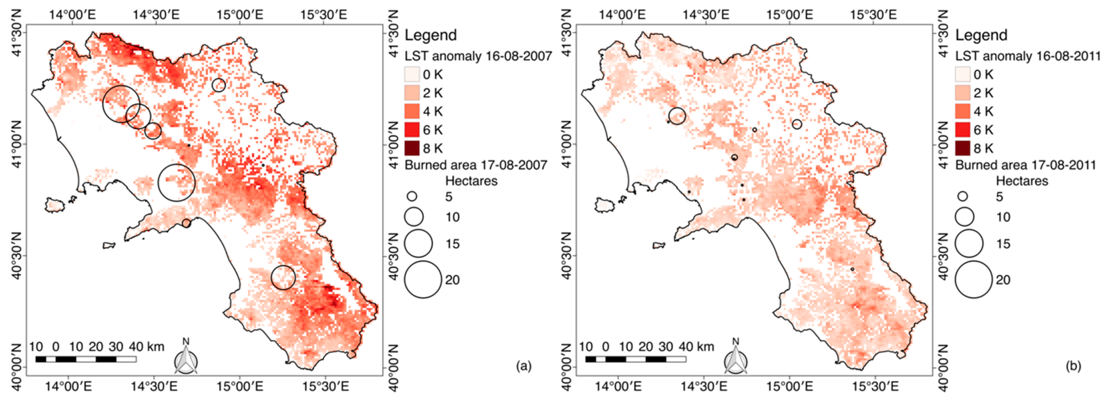
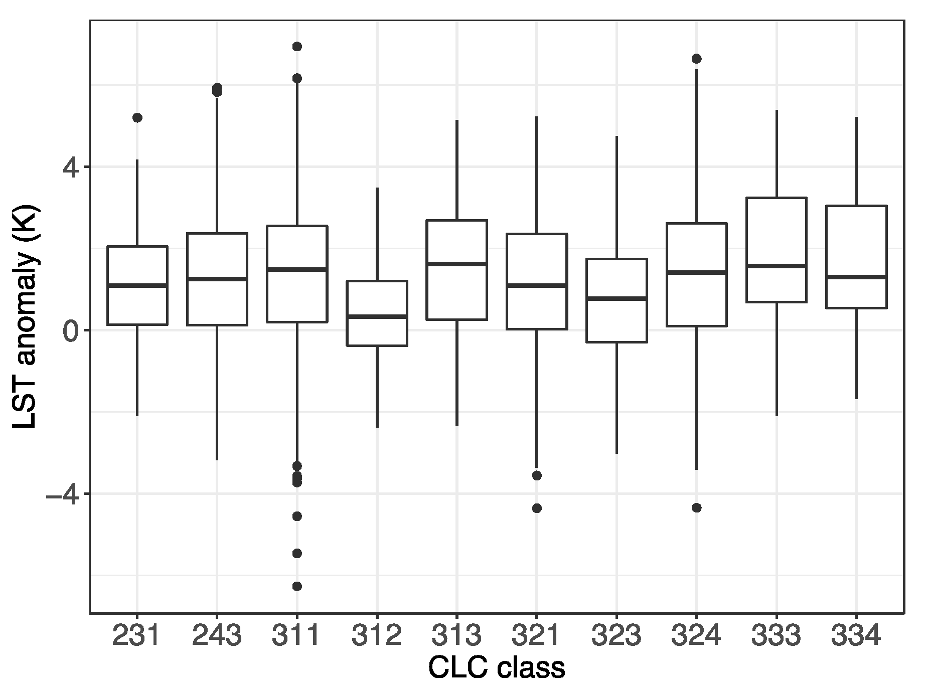
3.1. Evaluation of Land Surface Temperature Anomaly

LST in the study area exhibits significant inter-annual variability, as demonstrated by the two sample maps extracted from LST annual models of years 2007 and 2011 on the same date (Figure 3). However, absolute LST values are not indicative of deviations from a climatology. Indeed maps of LST anomaly on the same dates show significantly different spatial patterns as opposed to the corresponding maps of LST (Figure 4).
In the proposed sample dates, Figure 4 also reports fires occurred in the following day, represented with circles proportional to burned area. Fires occurring where a higher LST anomaly is reported result in a larger burned area, albeit such qualitative observations may vary with the chosen dates. Similar observations could be drawn for fire duration, but for the sake of brevity these are not reported herein.
Maps of LST anomaly were sampled at each fire location on the day previous to the event. Observed average LST anomaly is 1.3 K. 77% of fires occur when a positive LST anomaly is observed. On a monthly basis, this percentage varies between 69% and 88%, the only exception being December with 57%. A partial dependence of LST anomaly values from CLC classes is observed, with coniferous forest and sclerophyllous vegetation showing a wider proportion of fires occurring when a negative LST anomaly is recorded (Figure 5).

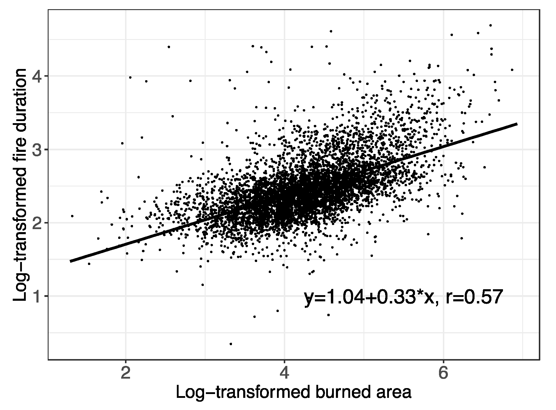
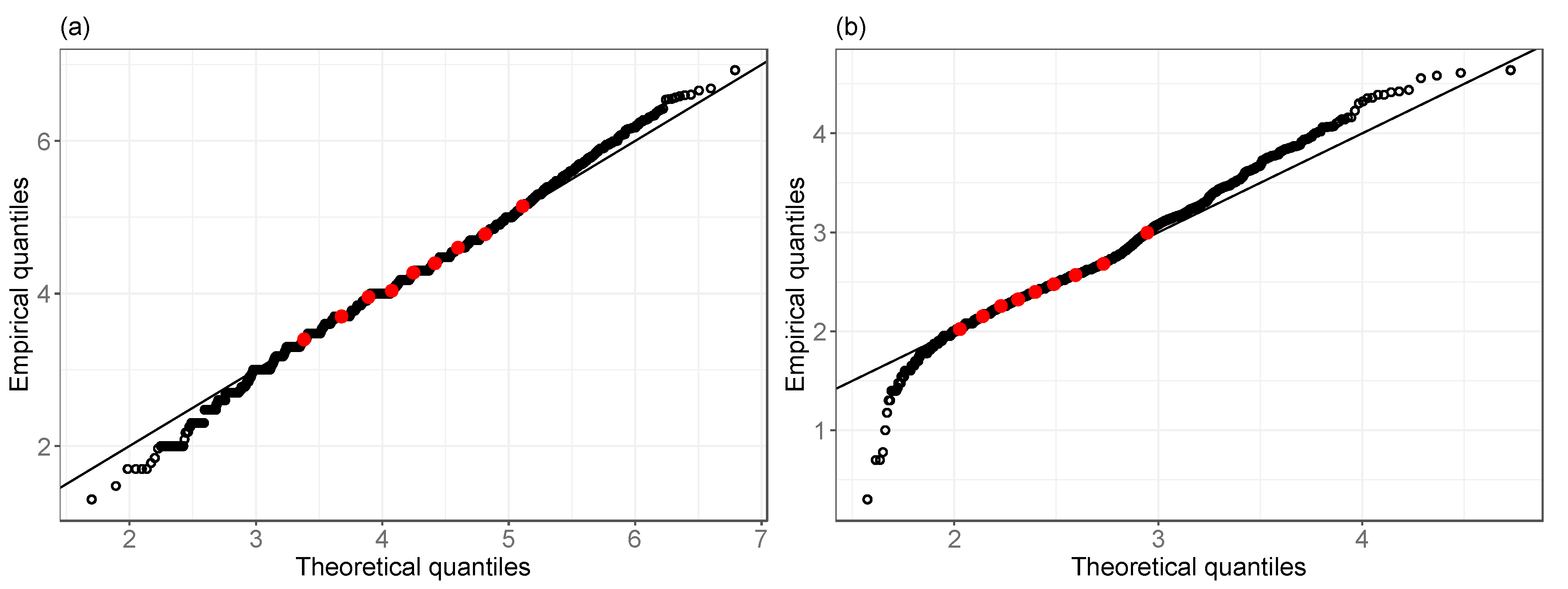
3.2. Statistical Models of Burned Area and Fire Duration

Burned area and fire duration range over several orders of magnitude and are strongly positively skewed. For this reason, they were preliminary scaled and converted to their base 10 logarithm, so as to have log-transformed positive values only. An initial investigation highlighted that log-transformed burned area and log-transformed fire duration show a linear correlation with a Pearson’s correlation coefficient of 0.57 (Figure 6). While clearly related, the relative weakness of this correlation confirms that the two quantities are not redundant.
Figure 7 reports scatterplots of log-transformed burned area and log-transformed fire duration against corresponding LST anomaly. Pearson’s correlation coefficients are 0.15 and 0.16 respectively, confirming that the observed large variability in these fire characteristics cannot be explained by the sole LST anomaly and indeed no trends can be clearly identified. To facilitate interpretation, data were subdivided in ten decile bins of LST anomaly and mean log-transformed burned area and log-transformed fire duration were calculated in each bin. Results plotted in Figure 8 show clearer trends, with mean log-transformed burned area increasing with increasing LST anomaly, confirming that the latter might be a covariate of this fire characteristic. A similar consideration may be drawn for log-transformed fire duration.
The parametric probability distributions identified in Section 2.4 were fitted to log-transformed burned area and log-transformed fire duration using the maximum goodness-of-fit method. The corresponding Anderson-Darling distance reported in Table 3 show that log-transformed burned area is more closely described by a normal distribution, whereas log-transformed fire duration is closer to a GEV distribution. The corresponding Q-Q plots are reported in Figure 9.

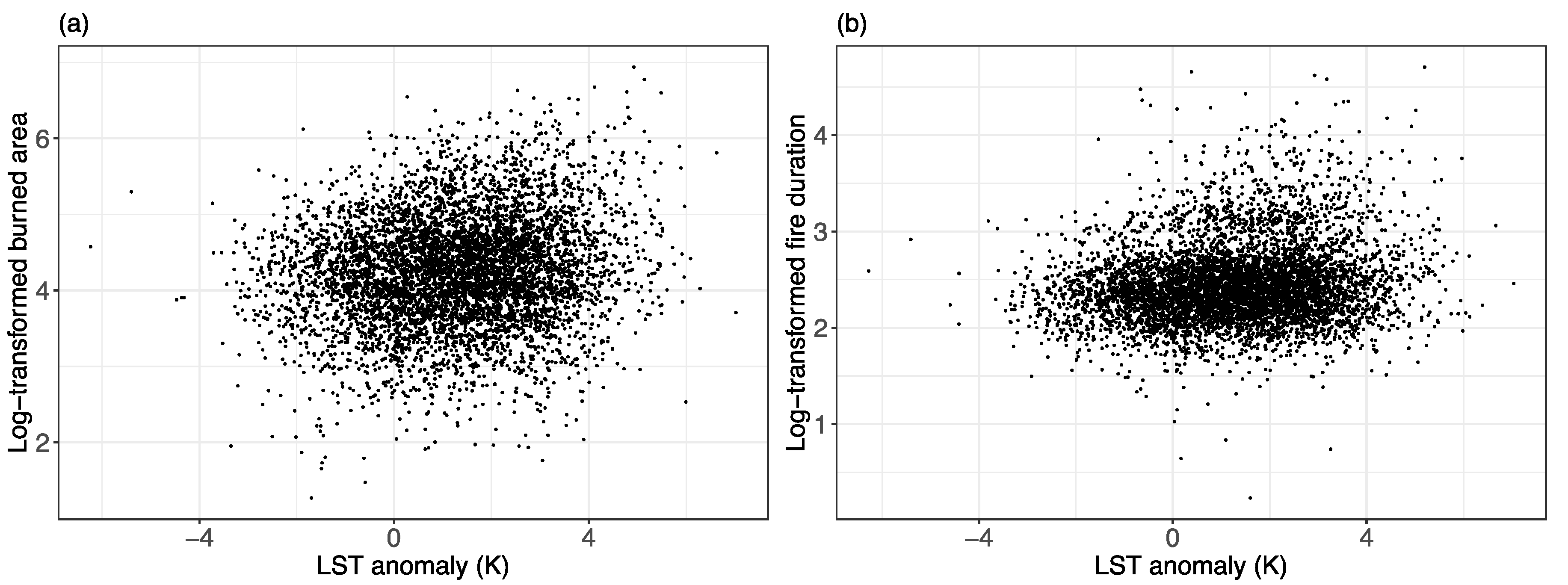
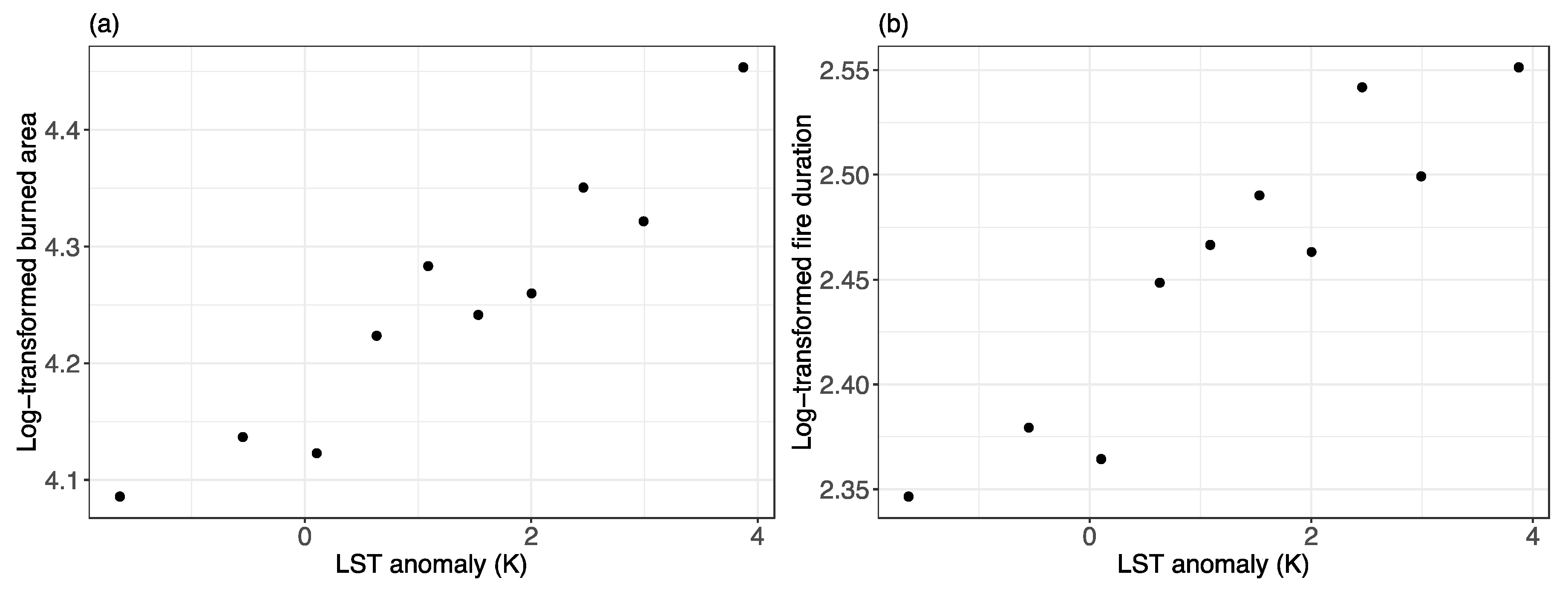
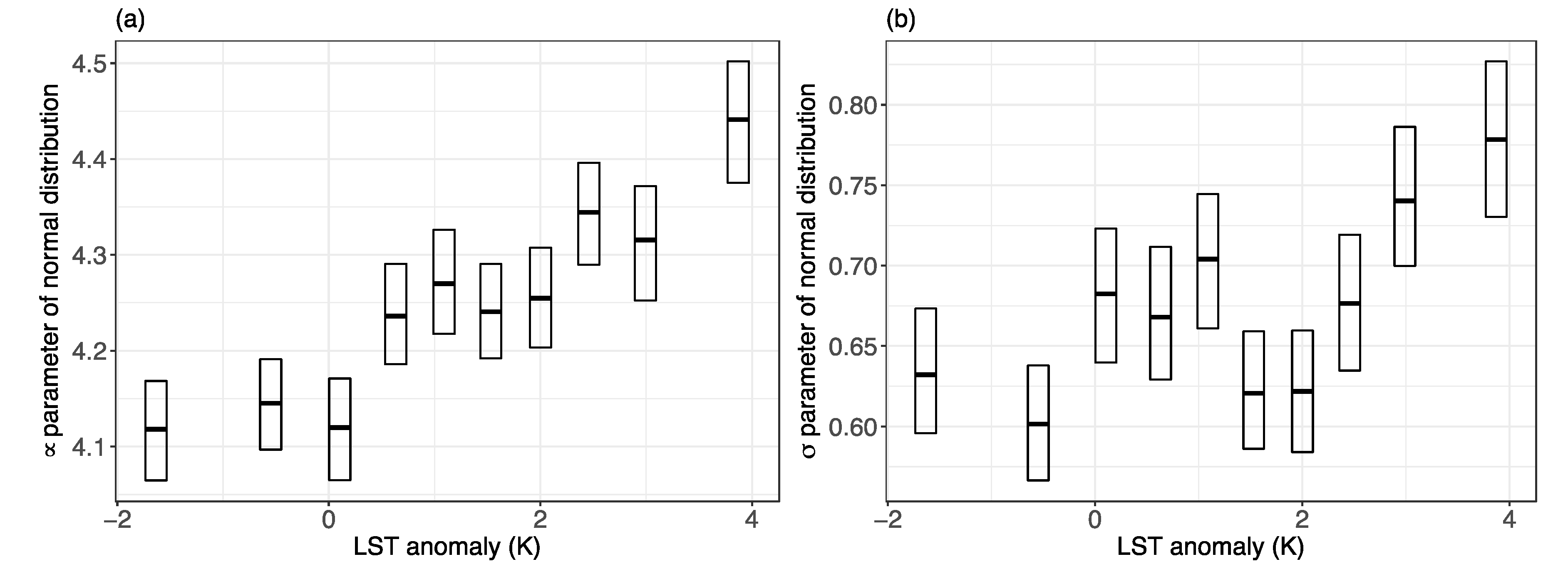
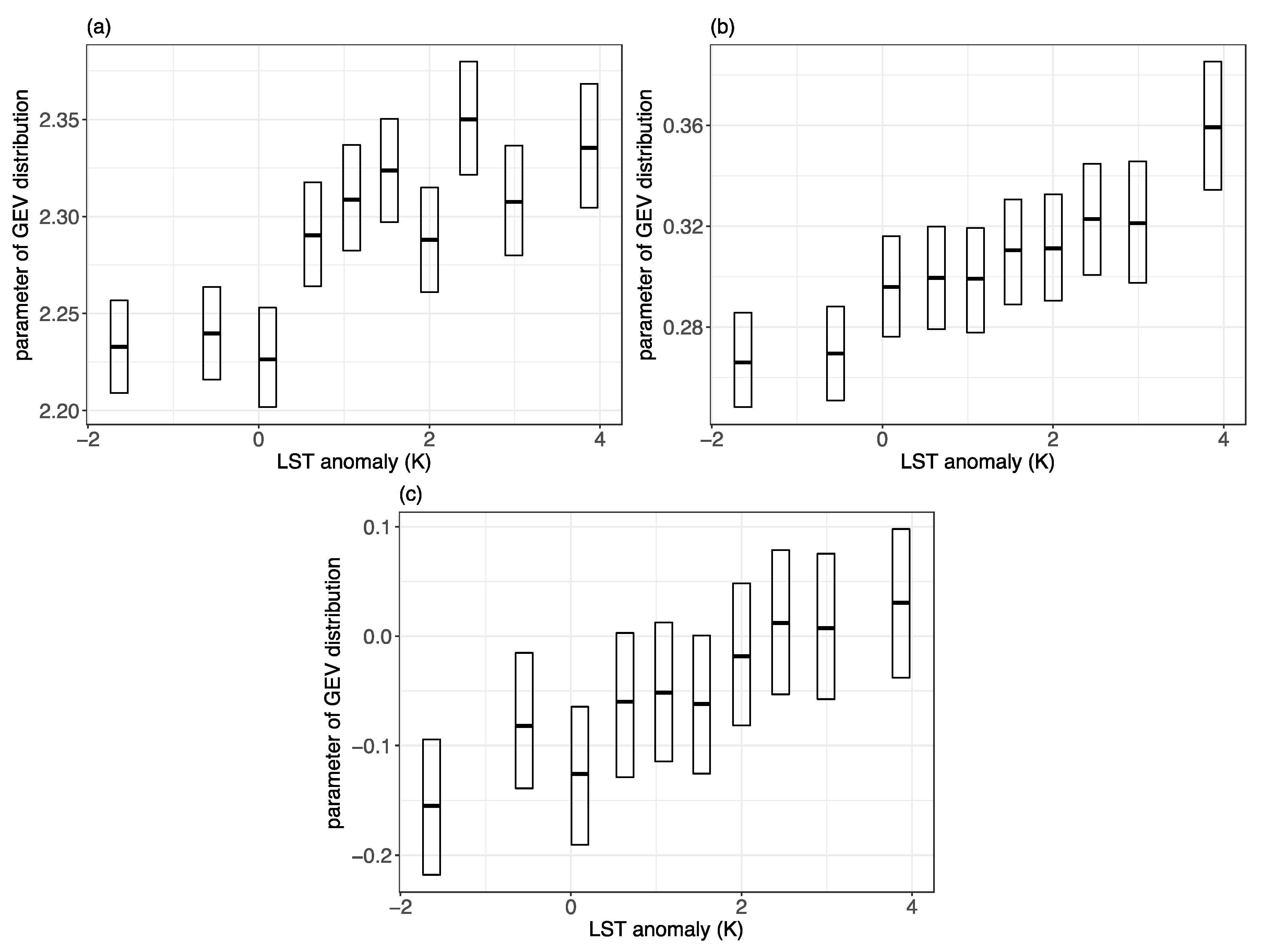
3.3. Conditional Distribution of Burned Area and Fire Duration

Parameters of the normal distribution of log-transformed burned area show a clear trend against LST anomaly (Figure 10). The sum of the likelihoods of the ten models fitted to burned area data in each bin was compared against the likelihood of the model describing the entire dataset by means of a likelihood ratio test. The null hypothesis in which the ten distributions are identical to the distribution describing all burned area data collectively was rejected at a significance level of p < 0.05. A similar result was observed with the GEV distribution of log-transformed fire duration, where the location a, scale b and shape s exhibit a clear trend with LST anomaly (Figure 11) and the null hypothesis is rejected with p < 0.05.
The retrieved conditional distributions (ten for each of the two fire characteristics, one in each of LST anomaly decile bins) were used to calculate the probability of fires larger than 27.8 ha (95th percentile of burned area) and the probability of fires lasting more than 27.5 hours (95th percentile of fire duration). Resulting plots (Figure 12) show that probability of large fires ranges from 1.8% in the first LST anomaly decile to 9.9% in the tenth decile, that is when LST anomaly increases from −1.6 to 3.9 K. Analogously, probability of fires lasting more than 27.5 h ranges from 0.4% to 8.9%.

4. Discussion

A clear relationship exists in several ecosystems between forest fire activity and meteorological forcing [11,12,13,14,15,16]. Prolonged absence of rainfall and increased air temperatures, while creating the preconditions for forest fires, push vegetation towards water stress conditions to which it responds by reducing transpiration. This leads in turn to an increase of vegetation temperature, a phenomenon that can be detected by remote sensing measurements in the thermal infrared [28,29,30,31,32,33,34,35]. Rather than modelling a direct dependence, this study hypothesized that remote observations of LST and more specifically deviations of LST values from a climatology, could be a covariate of burned area and fire duration of individual fires. Intuitively, prolonged events could eventually lead to larger burnt scars. Indeed, a correlation was found between log-transformed burned area and log-transformed fire duration (Figure 6), albeit its relative weakness supports the idea that these two quantities could be studied separately.
This research faced two substantial challenges. The first one was the identification of a suitable probability distribution model describing burned area and fire duration data in the study area. Several models are reported in cited literature [93,94,95,96,97,98,99,100] and indeed the diversity of these results highlights that no one single model can be identified to describe fire size distribution globally and that a model should be adopted on a per-study basis [99,101]. Among those tested herein, normal appears to be the closest fitting model for log-transformed burned area and GEV for log-transformed fire duration. In both circumstances, the fitting was not perfect towards the tails, as demonstrated by the relatively high Anderson-Darling distance (Table 3) and by the Q-Q plots (Figure 9). Indeed, the final extent of a fire and its duration are contributed by a large number of factors related to topography, land cover, climate, weather and anthropic action. The complex and varied landscape in the study area, with significant variations of population density, topography, land use/land cover and land management practices across its extent, created a unique combination of factors shaping the probability distributions of fire characteristics that is not properly captured by the tested models.
The second challenge was the construction of a climatology of LST to use as a basis for the evaluation of the LST anomaly. The phenomenon to be indirectly detected as a deviation from the LST climatology is the reduction in stomatal conductance due to plant water stress. The need to acknowledge for its intra-annual variability excluded the opportunity to identify a seasonal mean on any base that is not over short periods of time. Indeed, the availability of daily diurnal Aqua-MODIS measurements over fifteen years allowed the calculation of an LST climatology on a daily basis. Rather than a daily average, the latter was the result of the modelling of the time series by means of the HANTS algorithm. This approach has the advantage to retain seasonal variability while filtering out disturbance sources such as undetected cloud contamination, which induce a bias by reducing the detected temperature and the varying observation geometry [89].
HANTS algorithm was also used to model annual LST series individually. This led to the definition of the LST anomaly as a deviation of the LST annual model from the LST climatology. While the use of the LST annual model instead of current measurements might hinder the detection of LST variations occurring over a short period of time, this approach has the advantage of still detecting the build-up of the LST anomaly throughout the dry season while leveraging the named effects of observation geometry and residual cloud contamination [88].
The LST climatology and the LST annual models were constructed using the same HANTS parameters, with the only exception of FET (Table 2). The need for a more relaxed FET in the LST climatology was justified by the need to account for the inter-annual variability of LST. While affecting the shape of the modelled curve, a lower FET would clearly determine a climatology characterized by generally higher LST values. The value of FET = 6 K was identified as a compromise between the need of constructing an LST climatology of general validity while still rejecting cloud-contaminated data in both cooler and hotter years.
Fire data were intersected with maps of LST anomaly and each fire was associated with the LST anomaly value recorded at fire location on the day previous to the event. The underlying idea is that LST data is produced in near-real-time by ground receiving stations, allowing the mapping of fire danger forecast for the following day. The way LST anomaly was defined in this paper, that is as a deviation of LST annual model from LST climatology as opposed to the deviation of the actual MYD11A1 estimate, implies a slow day-to-day variation of LST anomaly. This in turn increases the temporal validity of produced LST anomaly maps up to a certain extent. Checking the effect of sampling in time at more days before the event was beyond the objectives of this research. However it is here anticipated that tests performed on LST anomalies recorded five days before the event led to results similar to those reported herein.
Observed average LST anomaly is 1.3 K, while 23% of fires occur with a negative LST anomaly. The distribution of LST anomaly appears to be partially dependent on land cover class as reported in Figure 5. Negative values are proportionally more prevalent in coniferous forest and sclerophyllous vegetation than in other land cover classes. The observation of this dependence was expected from literature review (e.g., [63,65]) and does not affect the quality of further findings. Indeed, evaluations of burned area and fire duration were performed conditional to LST anomaly, that is leveraging out all other parameters. In effect, other factors such as accessibility of the zone, availability and efficacy of the fire extinguishing means and the winds can heavily influence the occurrence of fires, the final burned area and event duration regardless of the previous LST anomaly, either positive or negative
This study demonstrated the informative content of time series of LST through the observation that LST anomaly is a covariate of burned area and fire duration. Fire data were grouped in ten decile bins of the associated LST anomaly values and the parameters of the identified distributions along with their 95% confidence interval were evaluated in each of them. The choice of the number of bins was initially tested with a trial and error approach, towards the identification of a compromise between the clarity of observed trends and the amplitude of the distribution parameters confidence interval. As similar results were observed across a range from five to twenty bins, for the sake of objectiveness in the approach the number of ten was chosen as the most appropriate.
Mean and variance of the normal distribution describing log-transformed burned area both tend to increase with increasing LST anomaly values (Figure 10), likewise the location, scale and shape parameters of the GEV distribution describing log-transformed fire duration (Figure 11). A likelihood ratio test confirmed that probability distribution models of burned area and fire duration conditional to LST anomaly are collectively significantly different than the models describing the entire dataset. Along with the observed trends in parameters values, this result confirms the stated hypothesis that LST anomaly as defined in this paper is a meaningful variable contributing to fire danger, that is that this quantity, along with its time-dependent nature, may be used pairwise other relevant parameters towards the statistical modelling of burned area and fire duration.
As a consequence of the variation of burned area and fire duration probability distributions conditional to LST anomaly, it is possible to plot and interpret how the probability of extreme events evolves with increasing LST anomaly values. Indeed, end users such as forest managers and civil protection agencies are particularly interested in these probabilities to drive their preparedness activities [103]. The models constructed in the ten decile bins of LST anomaly demonstrate that the probability of a forest fire to result in a total burned area exceeding a given threshold (in our example, the 95th percentile of the dataset) significantly increases with increasing LST values (Figure 12a). A similar result was found for fire duration (Figure 12b), supporting the idea that maps of LST anomaly such as those in Figure 4 are useful to depict the contribution of LST to fire danger.

5. Conclusions

Vegetation response to meteorological factors contributing to fire danger—prolonged absence of rainfall and high air temperature—results in an increase of LST that can be detected by remote sensing measurements in the thermal infrared as a deviation from climatological values. This paper demonstrates that such LST anomalies are a covariate of forest fires burned area and duration. While several studies demonstrated how a wide number of both static and dynamic factors related to topography, land cover, climate, weather and anthropic activity affect the probability distribution of these two fire characteristics, to the best of authors’ knowledge no previous research was conducted to investigate the role of satellite measurements of LST.
The initial hypothesis was addressed by first identifying probability distributions functions describing available fire data. Among those tested, log-transformed burned area is closer to a normal distribution, while log-transformed fire duration is closer to a generalized extreme value distribution. The HANTS algorithm was then used to process time series of diurnal Aqua-MODIS LST measurements and construct a climatology against which anomalies of LST were quantified. Finally, parameters of the identified distributions conditional to LST anomaly where then evaluated, showing clear trends.
The observed variation of burned area and fire duration distributions conditional to LST anomaly demonstrate that increasing positive deviations of LST from the expected seasonal value correspond to an increasing probability of extreme events, that is, of the final fire extent and duration exceeding a given threshold. This observation clearly identifies a practical mean to interpret maps of LST anomaly. As opposed to typical fire danger rating systems based on meteorological data, this remote sensing quantity has the advantage of claiming a higher spatial resolution. It is here highlighted that the identified relationships are preconditioning in nature and do not predict actual fire occurrence. The latter is related to a different array of determinants relating to probability of a heat source leading to an ignition.
This analysis was performed ex post trough the evaluation of LST annual models against an LST climatology. This approach is observational in nature and not predictive. While the achievement of more generality of the proposed research would require investigations in a wider and diverse array of regions, the predictive capability of the developed approach still needs to be demonstrated. This was beyond the objectives of this research and will be the subject of further investigations.

Author Contributions

Conceptualization, C.M. and M.M.; methodology, C.M. and S.M.A.; validation, C.M. and M.M.; formal analysis, C.M. and S.M.A.; investigation, C.M. and M.M.; data curation, C.M.; writing—original draft preparation, C.M.; writing—review and editing, C.M., S.M.A. and M.M.; visualization, C.M.; supervision, M.M. All authors read and approved the manuscript.

Funding

This research received no external funding.

Acknowledgments

We are grateful to Carabinieri (Italian national gendarmerie) and to Dipartimento della Protezione Civile (Italian Civil Protection Department) for providing fire data. We acknowledge the relevant contribution of reviewers in improving this manuscript.

Conflicts of Interest

The authors declare no conflict of interest.

References

  1. Certini, G. Effects of fire on properties of forest soils: A review. Oecologia 2005, 143, 1–10. [Google Scholar] [CrossRef] [PubMed]
  2. Thonicke, K.; Venevsky, S.; Sitch, S.; Cramer, W. The role of fire disturbance for global vegetation dynamics: Coupling fire into a Dynamic Global Vegetation Model. Glob. Ecol. Biogeogr. 2008, 10, 661–677. [Google Scholar] [CrossRef]
  3. van der Werf, G.R.; Randerson, J.T.; Giglio, L.; Collatz, G.J.; Mu, M.; Kasibhatla, P.S.; Morton, D.C.; Defries, R.S.; Jin, Y.; van Leeuwen, T.T. Global fire emissions and the contribution of deforestation, savanna, forest, agricultural, and peat fires (1997–2009). Atmos. Chem. Phys. 2010, 10, 11707–11735. [Google Scholar] [CrossRef] [Green Version]
  4. Seidl, R.; Schelhaas, M.-J.; Rammer, W.; Verkerk, P.J. Increasing forest disturbances in Europe and their impact on carbon storage. Nat. Clim. Chang. 2014, 4, 806–810. [Google Scholar] [CrossRef] [PubMed] [Green Version]
  5. Harvey, B.J.; Donato, D.C.; Turner, M.G. High and dry: Post-fire tree seedling establishment in subalpine forests decreases with post-fire drought and large stand-replacing burn patches. Glob. Ecol. Biogeogr. 2016, 25, 655–669. [Google Scholar] [CrossRef]
  6. Viegas, D.X. (Ed.) Recent Forest Fire Related Accidents in Europe; Office for Official Publications of the European Communities: Luxembourg, 2009; ISBN 9789279146046. [Google Scholar]
  7. Reisen, F.; Duran, S.M.; Flannigan, M.; Elliott, C.; Rideout, K. Wildfire smoke and public health risk. Int. J. Wildland Fire 2015, 24, 1029–1044. [Google Scholar] [CrossRef]
  8. Montagné-Huck, C.; Brunette, M. Economic analysis of natural forest disturbances: A century of research. J. For. Econ. 2018, 32, 42–71. [Google Scholar] [CrossRef]
  9. Liu, Y.; Stanturf, J.; Goodrick, S. Trends in global wildfire potential in a changing climate. For. Ecol. Manag. 2010, 259, 685–697. [Google Scholar] [CrossRef]
  10. Frank, D.; Reichstein, M.; Bahn, M.; Thonicke, K.; Frank, D.; Mahecha, M.D.; Smith, P.; van der Velde, M.; Vicca, S.; Babst, F.; et al. Effects of climate extremes on the terrestrial carbon cycle: Concepts, processes and potential future impacts. Glob. Chang. Biol. 2015, 21, 2861–2880. [Google Scholar] [CrossRef] [PubMed] [Green Version]
  11. Williams, A.P.; Abatzoglou, J.T. Recent advances and remaining uncertainties in resolving past and future climate effects on global fire activity. Curr. Clim. Chang. Rep. 2016, 2, 1–14. [Google Scholar] [CrossRef]
  12. Seidl, R.; Thom, D.; Kautz, M.; Martin-Benito, D.; Peltoniemi, M.; Vacchiano, G.; Wild, J.; Ascoli, D.; Petr, M.; Honkaniemi, J.; et al. Forest disturbances under climate change. Nat. Clim. Chang. 2017, 7, 395–402. [Google Scholar] [CrossRef] [PubMed] [Green Version]
  13. Lindner, M.; Maroschek, M.; Netherer, S.; Kremer, A.; Barbati, A.; Garcia-Gonzalo, J.; Seidl, R.; Delzon, S.; Corona, P.; Kolström, M.; et al. Climate change impacts, adaptive capacity, and vulnerability of European forest ecosystems. For. Ecol. Manag. 2010, 259, 698–709. [Google Scholar] [CrossRef]
  14. Gudmundsson, L.; Rego, F.C.; Rocha, M.; Seneviratne, S.I. Predicting above normal wildfire activity in southern Europe as a function of meteorological drought. Environ. Res. Lett. 2014, 9, 084008. [Google Scholar] [CrossRef]
  15. Trenberth, K.E.; Dai, A.; van der Schrier, G.; Jones, P.D.; Barichivich, J.; Briffa, K.R.; Sheffield, J. Global warming and changes in drought. Nat. Clim. Chang. 2014, 4, 17–22. [Google Scholar] [CrossRef]
  16. Zhang, K.; Kimball, J.S.; Nemani, R.R.; Running, S.W.; Hong, Y.; Gourley, J.J.; Yu, Z. Vegetation greening and climate change promote multidecadal rises of global land evapotranspiration. Sci. Rep. 2015, 5, 15956. [Google Scholar] [CrossRef] [PubMed]
  17. Douglass, J.E. Effects of species and arrangement of forests on evapotranspiration. In Proceedings of the International Symposium on Forest Hydrology; Sopper, W.E., Lull, H.W., Eds.; Pergamon: New York, NY, USA, 1967; pp. 451–461. [Google Scholar]
  18. Swift, L.W.; Swank, W.T.; Mankin, J.B.; Luxmoore, R.J.; Goldstein, R.A. Simulation of evapotranspiration and drainage from mature and clear-cut deciduous forests and young pine plantation. Water Resour. Res. 1975, 11, 667–673. [Google Scholar] [CrossRef]
  19. Arnold, J.G.; Srinivasan, R.; Muttiah, R.S.; Williams, J.R. Large area hydrologic modeling and assessment—Part I: Model development. J. Am. Water Resour. Assoc. 1998, 34, 73–89. [Google Scholar] [CrossRef]
  20. Viney, N.R. A review of fine fuel moisture modelling. Int. J. Wildland Fire 1991, 1, 215–234. [Google Scholar] [CrossRef]
  21. Aguado, I.; Chuvieco, E.; Borén, R.; Nieto, H. Estimation of dead fuel moisture content from meteorological data in Mediterranean areas. Applications in fire danger assessment. Int. J. Wildland Fire 2007, 16, 390–397. [Google Scholar] [CrossRef] [Green Version]
  22. Liu, Y. Responses of dead forest fuel moisture to climate change. Ecohydrology 2017, 10, e1760. [Google Scholar] [CrossRef]
  23. Keetch, J.J.; Byram, G.M. A Drought Index for Forest Fire Control; U.S. Department of Agriculture, Forest Service, Southeastern Forest Experiment Station: Asheville, NC, USA, 1968.
  24. Weber, L.; Nkemdirim, L. Palmer’s drought indices revisited. Geogr. Ann. Ser. A Phys. Geogr. 1998, 80, 153–172. [Google Scholar] [CrossRef]
  25. Pellizzaro, G.; Cesaraccio, C.; Duce, P.; Ventura, A.; Zara, P. Relationships between seasonal patterns of live fuel moisture and meteorological drought indices for Mediterranean shrubland species. Int. J. Wildland Fire 2007, 16, 232–241. [Google Scholar] [CrossRef]
  26. Merzouki, A.; Leblon, B. Mapping fuel moisture codes using MODIS images and the Getis statistic over western Canada grasslands. Int. J. Remote Sens. 2011, 32, 1619–1634. [Google Scholar] [CrossRef]
  27. Arpaci, A.; Eastaugh, C.S.; Vacik, H. Selecting the best performing fire weather indices for Austrian ecoregions. Theor. Appl. Climatol. 2013, 114, 393–406. [Google Scholar] [CrossRef] [PubMed] [Green Version]
  28. Hsiao, T.C. Plant responses to water stress. Annu. Rev. Plant Physiol. 1973, 24, 519–570. [Google Scholar] [CrossRef]
  29. Schulze, E.-D.; Lange, O.L.; Kappen, L.; Buschbom, U.; Evenari, M. Stomatal responses to changes in temperature at increasing water stress. Planta 1973, 110, 29–42. [Google Scholar] [CrossRef] [PubMed]
  30. Zweifel, R.; Rigling, A.; Dobbertin, M. Species-specific stomatal response of trees to drought—A link to vegetation dynamics? J. Veg. Sci. 2009, 20, 442–454. [Google Scholar] [CrossRef]
  31. Jackson, R.D.; Idso, S.B.; Reginato, R.J.; Pinter, P.J. Canopy temperature as a crop water stress indicator. Water Resour. Res. 1981, 17, 1133–1138. [Google Scholar] [CrossRef]
  32. Nemani, R.R.; Running, S.W. Estimation of regional surface resistance to evapotranspiration from NDVI and thermal-IR AVHRR data. J. Appl. Meteorol. 1989, 28, 276–284. [Google Scholar] [CrossRef]
  33. Kalma, J.D.; McVicar, T.R.; McCabe, M.F. Estimating land surface evaporation: A review of methods using remotely sensed surface temperature data. Surv. Geophys. 2008, 29, 421–469. [Google Scholar] [CrossRef]
  34. Karnieli, A.; Agam, N.; Pinker, R.T.; Anderson, M.; Imhoff, M.L.; Gutman, G.G.; Panov, N.; Goldberg, A. Use of NDVI and land surface temperature for drought assessment: Merits and limitations. J. Clim. 2010, 23, 618–633. [Google Scholar] [CrossRef]
  35. Liu, Y.; Wu, C.; Peng, D.; Xu, S.; Gonsamo, A.; Jassal, R.S.; Altaf Arain, M.; Lu, L.; Fang, B.; Chen, J.M. Improved modeling of land surface phenology using MODIS land surface reflectance and temperature at evergreen needleleaf forests of central North America. Remote Sens. Environ. 2016, 176, 152–162. [Google Scholar] [CrossRef]
  36. Dimitrakopoulos, A.P.; Papaioannou, K.K. Flammability assessment of Mediterranean forest fuels. Fire Technol. 2001, 37, 143–152. [Google Scholar] [CrossRef]
  37. Pellizzaro, G.; Duce, P.; Ventura, A.; Zara, P. Seasonal variations of live moisture content and ignitability in shrubs of the Mediterranean Basin. Int. J. Wildland Fire 2007, 16, 633–641. [Google Scholar] [CrossRef]
  38. Chuvieco, E.; Aguado, I.; Jurdao, S.; Pettinari, M.L.; Yebra, M.; Salas, J.; Hantson, S.; de la Riva, J.; Ibarra, P.; Rodrigues, M.; et al. Integrating geospatial information into fire risk assessment. Int. J. Wildland Fire 2014, 23, 606–619. [Google Scholar] [CrossRef] [Green Version]
  39. Rossa, C.G.; Veloso, R.; Fernandes, P.M. A laboratory-based quantification of the effect of live fuel moisture content on fire spread rate. Int. J. Wildland Fire 2016, 25, 569–573. [Google Scholar] [CrossRef]
  40. Leblon, B. Monitoring forest fire danger with remote sensing. Nat. Hazards 2005, 35, 343–359. [Google Scholar] [CrossRef]
  41. Chowdhury, E.H.; Hassan, Q.K. Operational perspective of remote sensing-based forest fire danger forecasting systems. ISPRS J. Photogramm. Remote Sens. 2014, 104, 224–236. [Google Scholar] [CrossRef]
  42. Sobrino, J.A.; Del Frate, F.; Drusch, M.; Jiménez-Muñoz, J.C.; Manunta, P.; Regan, A. Review of thermal infrared applications and requirements for future high-resolution sensors. IEEE Trans. Geosci. Remote Sens. 2016, 54, 2963–2972. [Google Scholar] [CrossRef]
  43. Chuvieco, E.; Cocero, D.; Riaño, D.; Martin, P.; Martínez-Vega, J.; De La Riva, J.; Pérez, F. Combining NDVI and surface temperature for the estimation of live fuel moisture content in forest fire danger rating. Remote Sens. Environ. 2004, 92, 322–331. [Google Scholar] [CrossRef] [Green Version]
  44. Jang, J.; Viau, A.A.; Anctil, F. Thermal-water stress index from satellite images. Int. J. Remote Sens. 2006, 27, 1619–1639. [Google Scholar] [CrossRef]
  45. Chowdhury, E.H.; Hassan, Q.K. Development of a new daily-scale forest fire danger forecasting system using remote sensing data. Remote Sens. 2015, 7, 2431–2448. [Google Scholar] [CrossRef]
  46. Tien Bui, D.; Le, K.-T.; Nguyen, V.; Le, H.; Revhaug, I. Tropical forest fire susceptibility mapping at the Cat Ba National Park Area, Hai Phong City, Vietnam, using GIS-based kernel logistic regression. Remote Sens. 2016, 8, 347. [Google Scholar] [CrossRef]
  47. Yu, B.; Chen, F.; Li, B.; Wang, L.; Wu, M. Fire risk prediction using remote sensed products: A case of Cambodia. Photogramm. Eng. Remote Sens. 2017, 83, 19–25. [Google Scholar] [CrossRef]
  48. Abdollahi, M.; Islam, T.; Gupta, A.; Hassan, Q.K. An advanced forest fire danger forecasting system: Integration of remote sensing and historical sources of ignition data. Remote Sens. 2018, 10, 923. [Google Scholar] [CrossRef]
  49. Vidal, A.; Pinglo, F.; Durand, H.; Devaux-Ros, C.; Maillet, A. Evaluation of a temporal fire risk index in mediterranean forests from NOAA thermal IR. Remote Sens. Environ. 1994, 49, 296–303. [Google Scholar] [CrossRef]
  50. Nolan, R.H.; Resco de Dios, V.; Boer, M.M.; Caccamo, G.; Goulden, M.L.; Bradstock, R.A. Predicting dead fine fuel moisture at regional scales using vapour pressure deficit from MODIS and gridded weather data. Remote Sens. Environ. 2016, 174, 100–108. [Google Scholar] [CrossRef] [Green Version]
  51. Dasgupta, S.; Qu, J.J.; Hao, X. Design of a susceptibility index for fire risk monitoring. IEEE Geosci. Remote Sens. Lett. 2006, 3, 140–144. [Google Scholar] [CrossRef]
  52. Veraverbeke, S.; Verstraeten, W.W.; Lhermitte, S.; Van De Kerchove, R.; Goossens, R. Assessment of post-fire changes in land surface temperature and surface albedo, and their relation with fire-burn severity using multitemporal MODIS imagery. Int. J. Wildland Fire 2012, 21, 243–256. [Google Scholar] [CrossRef]
  53. Vlassova, L.; Pérez-Cabello, F.; Mimbrero, M.R.; Llovería, R.M.; García-Martín, A. Analysis of the relationship between land surface temperature and wildfire severity in a series of Landsat images. Remote Sens. 2014, 6, 6136–6162. [Google Scholar] [CrossRef]
  54. Quintano, C.; Fernández-Manso, A.; Calvo, L.; Marcos, E.; Valbuena, L. Land surface temperature as potential indicator of burn severity in forest Mediterranean ecosystems. Int. J. Appl. Earth Obs. Geoinf. 2015, 36, 1–12. [Google Scholar] [CrossRef]
  55. Zheng, Z.; Zeng, Y.; Li, S.; Huang, W. A new burn severity index based on land surface temperature and enhanced vegetation index. Int. J. Appl. Earth Obs. Geoinf. 2016, 45, 84–94. [Google Scholar] [CrossRef]
  56. Quintano, C.; Fernandez-Manso, A.; Roberts, D.A. Burn severity mapping from Landsat MESMA fraction images and Land Surface Temperature. Remote Sens. Environ. 2017, 190, 83–95. [Google Scholar] [CrossRef]
  57. Chaparro, D.; Vall-llossera, M.; Piles, M.; Camps, A.; Rüdiger, C.; Riera-Tatché, R. Predicting the extent of wildfires using remotely sensed soil moisture and temperature trends. IEEE J. Sel. Top. Appl. Earth Obs. Remote Sens. 2016, 9, 2818–2829. [Google Scholar] [CrossRef]
  58. Manzo-Delgado, L.; Aguirre-Gómez, R.; Álvarez, R. Multitemporal analysis of land surface temperature using NOAA-AVHRR: Preliminary relationships between climatic anomalies and forest fires. Int. J. Remote Sens. 2004, 25, 4417–4424. [Google Scholar] [CrossRef]
  59. Pan, J.; Wang, W.; Li, J. Building probabilistic models of fire occurrence and fire risk zoning using logistic regression in Shanxi Province, China. Nat. Hazards 2016, 81, 1879–1899. [Google Scholar] [CrossRef]
  60. Matin, M.A.; Chitale, V.S.; Murthy, M.S.R.; Uddin, K.; Bajracharya, B.; Pradhan, S. Understanding forest fire patterns and risk in Nepal using remote sensing, geographic information system and historical fire data. Int. J. Wildland Fire 2017, 26, 276–286. [Google Scholar] [CrossRef]
  61. Viegas, D.X.; Viegas, M.T. A relationship between rainfall and burned area for portugal. Int. J. Wildland Fire 1994, 4, 11–16. [Google Scholar] [CrossRef]
  62. Falk, D.A.; Miller, C.; McKenzie, D.; Black, A.E. Cross-scale analysis of fire regimes. Ecosystems 2007, 10, 809–823. [Google Scholar] [CrossRef]
  63. Faivre, N.; Jin, Y.; Goulden, M.L.; Randerson, J.T. Controls on the spatial pattern of wildfire ignitions in Southern California. Int. J. Wildland Fire 2014, 23, 799–811. [Google Scholar] [CrossRef] [Green Version]
  64. Fernandes, P.M.; Monteiro-Henriques, T.; Guiomar, N.; Loureiro, C.; Barros, A.M.G. Bottom-up variables govern large-fire size in portugal. Ecosystems 2016, 19, 1362–1375. [Google Scholar] [CrossRef]
  65. Barrett, K.; Loboda, T.; McGuire, A.D.; Genet, H.; Hoy, E.; Kasischke, E. Static and dynamic controls on fire activity at moderate spatial and temporal scales in the Alaskan boreal forest. Ecosphere 2016, 7, e01572. [Google Scholar] [CrossRef] [Green Version]
  66. Faivre, N.R.; Jin, Y.; Goulden, M.L.; Randerson, J.T. Spatial patterns and controls on burned area for two contrasting fire regimes in Southern California. Ecosphere 2016, 7, e01210. [Google Scholar] [CrossRef]
  67. Littell, J.S.; Peterson, D.L.; Riley, K.L.; Liu, Y.; Luce, C.H. A review of the relationships between drought and forest fire in the United States. Glob. Chang. Biol. 2016, 22, 2353–2369. [Google Scholar] [CrossRef] [PubMed]
  68. Gustafson, E.J.; Shvidenko, A.Z.; Scheller, R.M. Effectiveness of forest management strategies to mitigate effects of global change in south-central Siberia. Can. J. For. Res. 2011, 41, 1405–1421. [Google Scholar] [CrossRef]
  69. Fischer, M.A.; Di Bella, C.M.; Jobbágy, E.G. Influence of fuel conditions on the occurrence, propagation and duration of wildland fires: A regional approach. J. Arid Environ. 2015, 120, 63–71. [Google Scholar] [CrossRef]
  70. Costafreda-Aumedes, S.; Cardil, A.; Molina, D.M.; Daniel, S.N.; Mavsar, R.; Vega-Garcia, C. Analysis of factors influencing deployment of fire suppression resources in Spain using artificial neural networks. iForest-Biogeosci. For. 2016, 9, 138–145. [Google Scholar] [CrossRef] [Green Version]
  71. Lasslop, G.; Kloster, S. Human impact on wildfires varies between regions and with vegetation productivity. Environ. Res. Lett. 2017, 12, 115011. [Google Scholar] [CrossRef] [Green Version]
  72. Julien, Y.; Sobrino, J.A.; Verhoef, W. Changes in land surface temperatures and NDVI values over Europe between 1982 and 1999. Remote Sens. Environ. 2006, 103, 43–55. [Google Scholar] [CrossRef]
  73. Stroppiana, D.; Antoninetti, M.; Brivio, P.A. Seasonality of MODIS LST over Southern Italy and correlation with land cover, topography and solar radiation. Eur. J. Remote Sens. 2014, 47, 133–152. [Google Scholar] [CrossRef] [Green Version]
  74. Khorchani, M.; Vicente-Serrano, S.M.; Azorin-Molina, C.; Garcia, M.; Martin-Hernandez, N.; Peña-Gallardo, M.; El Kenawy, A.; Domínguez-Castro, F. Trends in LST over the peninsular Spain as derived from the AVHRR imagery data. Glob. Planet. Chang. 2018, 166, 75–93. [Google Scholar] [CrossRef]
  75. Verhoef, W. Application of Harmonic Analysis of NDVI Time Series (HANTS). In Fourier Analysis of Temporal NDVI in the Southern African and American Continents; Azzali, S., Menenti, M., Eds.; DLO–Winand Staring Centre: Wageningen, The Netherlands, 1996; pp. 19–24. [Google Scholar]
  76. Roerink, G.J.; Menenti, M.; Verhoef, W. Reconstructing cloudfree NDVI composites using Fourier analysis of time series. Int. J. Remote Sens. 2000, 21, 1911–1917. [Google Scholar] [CrossRef]
  77. Hernandez, C.; Keribin, C.; Drobinski, P.; Turquety, S. Statistical modelling of wildfire size and intensity: A step toward meteorological forecasting of summer extreme fire risk. Ann. Geophys. 2015, 33, 1495–1506. [Google Scholar] [CrossRef] [Green Version]
  78. Ceccarelli, T.; Smiraglia, D.; Bajocco, S.; Rinaldo, S.; De Angelis, A.; Salvati, L.; Perini, L. Land cover data from Landsat single-date imagery: An approach integrating pixel-based and object-based classifiers. Eur. J. Remote Sens. 2013, 46, 699–717. [Google Scholar] [CrossRef]
  79. Modugno, S.; Balzter, H.; Cole, B.; Borrelli, P. Mapping regional patterns of large forest fires in Wildland–Urban Interface areas in Europe. J. Environ. Manag. 2016, 172, 112–126. [Google Scholar] [CrossRef] [PubMed]
  80. San-Miguel-Ayanz, J.; Durrant, T.; Boca, R.; Libertà, G.; Branco, A.; de Rigo, D.; Ferrari, D.; Maianti, P.; Artés Vivancos, T.; Schulte, E.; et al. Forest Fires in Europe, Middle East and North Africa 2016; Publications Office of the European Union: Luxembourg, 2017; ISBN 978-92-79-71292-0. [Google Scholar]
  81. Wan, Z. New refinements and validation of the collection-6 MODIS land-surface temperature/emissivity product. Remote Sens. Environ. 2014, 140, 36–45. [Google Scholar] [CrossRef]
  82. Xu, Y.; Shen, Y. Reconstruction of the land surface temperature time series using harmonic analysis. Comput. Geosci. 2013, 61, 126–132. [Google Scholar] [CrossRef]
  83. Van Nguyen, O.; Kawamura, K.; Trong, D.P.; Gong, Z.; Suwandana, E. Temporal change and its spatial variety on land surface temperature and land use changes in the Red River Delta, Vietnam, using MODIS time-series imagery. Environ. Monit. Assess. 2015, 187, 464. [Google Scholar] [CrossRef] [PubMed]
  84. Ackerman, S.A.; Holz, R.E.; Frey, R.; Eloranta, E.W.; Maddux, B.C.; McGill, M. Cloud detection with MODIS. Part II: Validation. J. Atmos. Ocean. Technol. 2008, 25, 1073–1086. [Google Scholar] [CrossRef]
  85. European Environment Agency. CLC2006 Technical Guidelines; Office for Official Publications of the European Communities: Luxembourg, 2007; ISBN 9789291679683. [Google Scholar]
  86. Menenti, M.; Azzali, S.; Verhoef, W.; van Swol, R. Mapping agroecological zones and time lag in vegetation growth by means of Fourier analysis of time series of NDVI images. Adv. Space Res. 1993, 13, 233–237. [Google Scholar] [CrossRef]
  87. Verhoef, W.; Menenti, M.; Azzali, S. A colour composite of NOAA-AVHRR-NDVI based on time series analysis (1981–1992). Int. J. Remote Sens. 1996, 17, 231–235. [Google Scholar] [CrossRef]
  88. Alfieri, S.M.; De Lorenzi, F.; Menenti, M. Mapping air temperature using time series analysis of LST: The SINTESI approach. Nonlinear Process. Geophys. 2013, 20, 513–527. [Google Scholar] [CrossRef]
  89. Menenti, M.; Malamiri, H.R.G.; Shang, H.; Alfieri, S.M.; Maffei, C.; Jia, L. Observing the response of terrestrial vegetation to climate variability across a range of time scales by time series analysis of land surface temperature. In Multitemporal Remote Sensing; Ban, Y., Ed.; Springer International Publishing: Cham, Switzerland, 2016; pp. 277–315. ISBN 978-3-319-47035-1. [Google Scholar]
  90. Roerink, G.J.; Menenti, M.; Soepboer, W.; Su, Z. Assessment of climate impact on vegetation dynamics by using remote sensing. Phys. Chem. Earth 2003, 28, 103–109. [Google Scholar] [CrossRef]
  91. FAO. Wildland Fire Management Terminology; Food and Agriculture Organization of the United Nations: Rome, Italy, 1986; ISBN 92-5-002420-7. [Google Scholar]
  92. Walding, N.G.; Williams, H.T.P.; McGarvie, S.; Belcher, C.M. A comparison of the US National Fire Danger Rating System (NFDRS) with recorded fire occurrence and final fire size. Int. J. Wildland Fire 2018, 27, 99–113. [Google Scholar] [CrossRef]
  93. Weber, M.G.; Stocks, B.J. Forest fires in the boreal forests of Canada. In Large Forest Fires; Moreno, J.M., Ed.; Backhuys Publishers: Leiden, The Netherlands, 1998; pp. 215–233. ISBN 978-90-7334-880-6. [Google Scholar]
  94. Haydon, D.T.; Friar, J.K.; Pianka, E.R. Fire-driven dynamic mosaics in the Great Victoria Desert, Australia. Landsc. Ecol. 2000, 15, 373–381. [Google Scholar] [CrossRef]
  95. Corral, Á.; Telesca, L.; Lasaponara, R. Scaling and correlations in the dynamics of forest-fire occurrence. Phys. Rev. E 2008, 77, 016101. [Google Scholar] [CrossRef] [PubMed]
  96. Baker, W.L. Landscape ecology and nature reserve design in the Boundary Waters Canoe Area, Minnesota. Ecology 1989, 70, 23–35. [Google Scholar] [CrossRef]
  97. Cumming, S.G. A parametric model of the fire-size distribution. Can. J. For. Res. 2001, 31, 1297–1303. [Google Scholar] [CrossRef]
  98. Moritz, M.A. Analyzing Extreme disturbance events: Fire in Los Padres national forest. Ecol. Appl. 1997, 7, 1252–1262. [Google Scholar] [CrossRef]
  99. Reed, W.J.; McKelvey, K.S. Power-law behaviour and parametric models for the size-distribution of forest fires. Ecol. Model. 2002, 150, 239–254. [Google Scholar] [CrossRef]
  100. Palma, C.D.; Cui, W.; Martell, D.L.; Robak, D.; Weintraub, A. Assessing the impact of stand-level harvests on the flammability of forest landscapes. Int. J. Wildland Fire 2007, 16, 584–592. [Google Scholar] [CrossRef]
  101. Cui, W.; Perera, A.H. What do we know about forest fire size distribution, and why is this knowledge useful for forest management? Int. J. Wildland Fire 2008, 17, 234–244. [Google Scholar] [CrossRef]
  102. Anderson, T.W.; Darling, D.A. A test of goodness of fit. J. Am. Stat. Assoc. 1954, 49, 765–769. [Google Scholar] [CrossRef]
  103. Preisler, H.K.; Brillinger, D.R.; Burgan, R.E.; Benoit, J.W. Probability based models for estimation of wildfire risk. Int. J. Wildland Fire 2004, 13, 133–142. [Google Scholar] [CrossRef]
Figure 1. Study area is Campania region, Italy (40°83′N, 14°13′E, 13595 km2).
Remotesensing 10 01777 g001
Figure 2. Aqua-MODIS LST data, LST annual model and LST climatology observed in year 2007 in pixel 40°50′40″N, 14°8′56″E.
Remotesensing 10 01777 g002
Figure 3. Sample maps of LST as derived from HANTS processing of annual time series in vegetated and recently burned areas (land cover classes in Table 1): 16 August 2007 (a); 16 August 2011 (b).
Remotesensing 10 01777 g003
Figure 4. Land surface temperature anomaly observed in vegetated and recently burned areas (land cover classes in Table 1) on 16 August 2007 with superimposed fires recorded on 17 August 2007 (a) and on 16 August 2011 with superimposed fires recorded on 17 August 2011 (b).
Remotesensing 10 01777 g004
Figure 5. Boxplot of observed LST anomaly in each CLC class (Table 1).
Remotesensing 10 01777 g005
Figure 6. Scatterplot of log-transformed fire duration against log-transformed burned area.
Remotesensing 10 01777 g006
Figure 7. Scatterplot of log-transformed burned area (a) and log-transformed fire duration (b) against LST anomaly.
Remotesensing 10 01777 g007
Figure 8. Variation of mean burned area (a) and mean fire duration (b) in ten deciles of land surface temperature anomaly.
Remotesensing 10 01777 g008
Figure 9. Q-Q plots of the normal distribution of log-transformed burned area (a) and of the generalized extreme value distribution of log-transformed fire duration (b). Red circles highlight the deciles of the distributions.
Remotesensing 10 01777 g009
Figure 10. Plots of µ (a) and σ (b) parameters of normal distribution of log-transformed burned area and their 95% confidence intervals, conditional to land surface temperature anomaly in 10 decile bins.
Remotesensing 10 01777 g010
Figure 11. Plot of location a (a), scale b (b) and shape s (c) parameters of generalized extreme value distribution of log-transformed fire duration and their 95% confidence intervals, conditional to LST anomaly in 10 decile bins.
Remotesensing 10 01777 g011
Figure 12. Estimated probability of burned area exceeding 27.8 ha, conditional to LST anomaly values in 10 decile bins (a); estimated probability of fire duration exceeding 27.5 h, conditional to LST anomaly values in 10 decile bins (b).
Remotesensing 10 01777 g012
Table 1. CORINE Land Cover (CLC) classes used to select fires used in subsequent analyses.
CLC CodeDescription
231Pastures
243Land principally occupied by agriculture, with significant areas of natural vegetation
244Agro-forestry areas
311Broad-leaved forest
312Coniferous forest
313Mixed forest
321Natural grassland
322Moors and heathland
323Sclerophyllous vegetation
324Transitional woodland shrub
333Sparsely vegetated areas
334Burnt areas
Table 2. Parameters used in HANTS algorithm to pre-process LST data.
HANTS ParametersLST Annual ModelsLST Climatology
Length of the base period (L)1 year1 year
Number of frequencies (M)33
Direction of outliers rejectionLoLo
Fit error tolerance (FET)4 K6 K
Degree of over-determinedness (DOD)Half of valid pointsHalf of valid points
Table 3. Anderson-Darling distance values for all tested distributions.
ModelLog-Transformed
Burned Area
Log-Transformed
Fire Duration
Normal9.269.5
Log-normal20.228.8
Exponential16621711
Gamma13.539.7
Generalized extreme value13.515.1
Weibull32.6245

