Seven Years of SMOS Sea Surface Salinity at High Latitudes: Variability in Arctic and Sub-Arctic Regions

 ,
,  ,
,  ,
,  , and
, and
Abstract
1. Introduction
2. Datasets
2.1. SMOS Brightness Temperatures: Level 1B Product
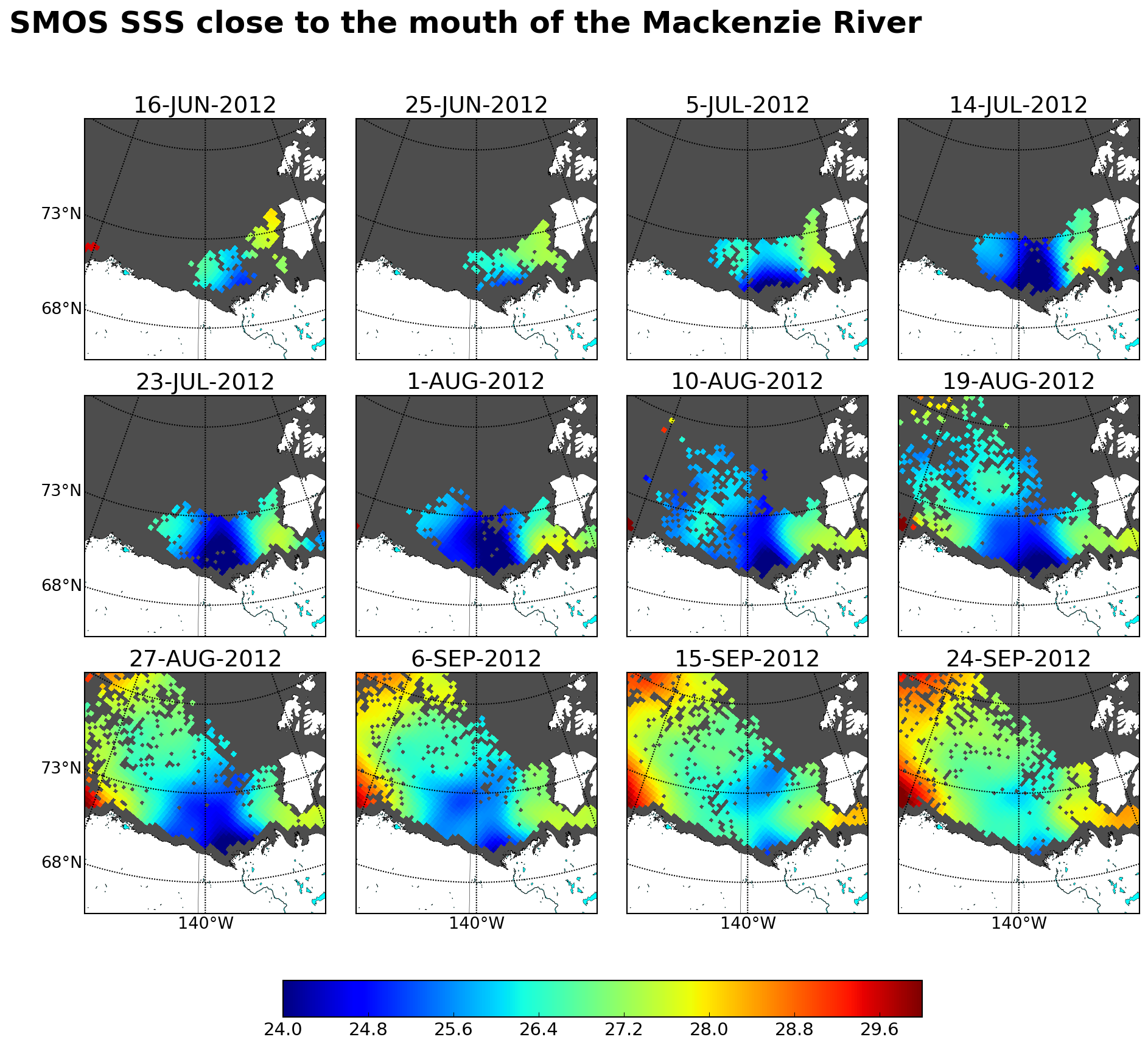
2.2. Argo Salinity
2.3. TARA Salinity
2.4. TSG Salinity Data
2.5. TOPAZ Salinity
2.6. Aquarius SSS L3 Maps
2.7. SMAP SSS L3 Maps
2.8. River Discharge In Situ Measurements
3. Methodology Used for the SMOS SSS Product Generation
- (a)
- Individual retrievals: The retrieval follows a non-Bayesian scheme, that is, for each SMOS a single value of SSS is retrieved.
- (b)
- Characterization of the systematic errors: All the SSS retrieved under the same acquisition conditions, i.e., the same geographical location, incidence and azimuth angles and satellite overpass direction (ascending/descending). throughout this seven-year period are accumulated in a SSS distribution. The systematic error associated to each acquisition condition is estimated by computing the central estimator of the corresponding SSS distributions. We use the mode of the distribution as the central estimator, i.e., as the SMOS climatological value for each specific acquisition condition. In this aspect, a relevant difference with respect to the official SMOS L2OS processor is that the used for the ESA SMOS L2OS SSS retrieval are previously corrected by Ocean Target Transformation (OTT) [44]. The OTT is computed as the mean of the difference between the measured and modeled s (applying the Geophysical Forward Model) at a particularly stable region of the ocean. We do not apply an OTT since systematic errors are already accounted for, point by point, with the new methodology.
- (c)
- Filtering criteria: The statistical properties of those SSS distributions are also used for filtering the non-accurate measurements. Two types of filters are applied to remove questionable values and outliers in the SSS retrievals: (i) all the SSS belonging to distributions having a large standard deviation (std larger than 10), defined by too few measurements (less than 100), or with a large skewness (larger than 1 in absolute value) or kurtosis (lower than 2) are all excluded (i.e., the distribution is marked as “bad” distribution, and all its salinities are discarded); and (ii) an additional outlier criterion is applied to the remaining retrieval values by further excluding any value that is farther than 10 (in absolute value) from the SMOS climatological value (see more details in [23]).
- (d)
- Computation of SMOS anomalies: The SMOS-debiased SSS anomalies are computed by subtracting to each individually retrieved SSS value (corresponding to a specific acquisition condition) the corresponding SMOS climatological value (computed as explained in (b)), thus effectively removing local biases, especially those produced by the land–sea (or ice–sea) contamination and permanent RFIs.
- (e)
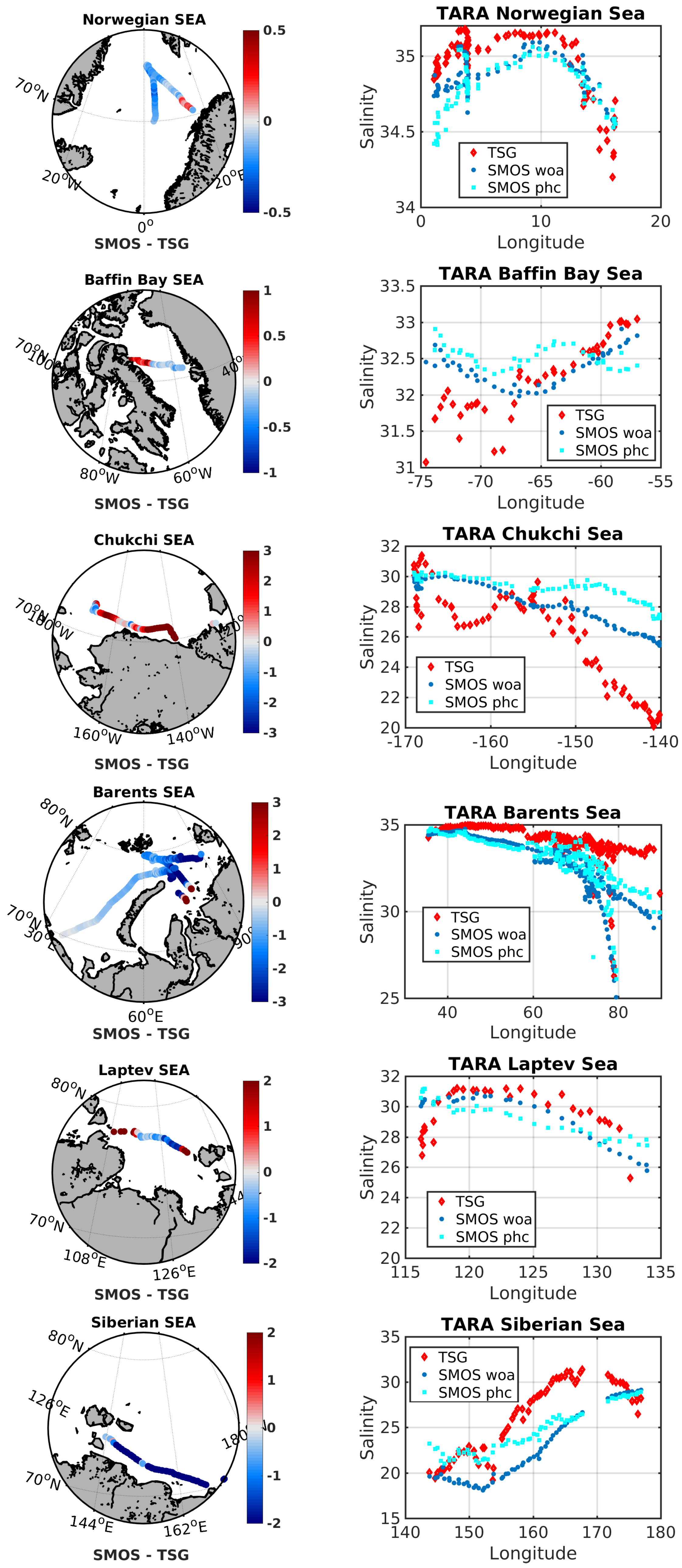
- Computation of SMOS SSS: In [23], the SMOS SSS are generated by adding an annual SSS reference (annual WOA SSS, [45]) to the SMOS anomalies. This is an issue for the SMOS SSS values of the Arctic Ocean, since there are many zones in the Arctic with very few measurements of SSS (as shown in the bottom-right plot of Figure 1), and any reference could provide non-accurate SSS values there. For this reason, before generating the seven years of SMOS SSS, we analyze two test datasets by using two annual references: WOA; and the Polar science center Hydrographic annual Climatology (PHC) (version 3) [46] which is the usual reference for Arctic regions. We assess the quality of these two datasets by comparing the resulting SMOS SSS products—the SMOS SSS computed from WOA annual reference (SMOS woa) and SMOS SSS computed from PHC (SMOS phc)—with TARA SSS. In Section 4.1, a full discussion of this assessment is given. The conclusions of these comparisons are summarized in Figure 2. SMOS SSS has lower RMS with respect to TARA SSS than the corresponding annual references used for its generation (i.e., the blue and red lines are below the green and black lines, respectively, except in Buffin Bay where the SMOS-PHC has slightly larger RMS than the PHC product). The actual RMS values, together with the bias and standard deviation values, can be found in Table 1. However, many regions in the Arctic Ocean present large RMS values. These regions correspond to the areas where few or no in situ data were taken into account in the generation of the annual reference. In Section 4.1, we describe this analysis in more detail. Since both references provide similar results (WOA is slightly better), we use WOA for the generation of SMOS SSS product to be coherent with the global SMOS SSS product distributed by BEC.
- (f)
- Objectively analyzed maps: Objectively analyzed nine-day SSS maps at 25-km resolution are generated daily. In [23], the same correlation radii used for the computation of WOA products were proposed for the generation of the SMOS SSS products: 321 km, 267 km, and 175 km (see [45]). These correlation radii do not seem to be the most appropriate for describing the dynamics in the Arctic region [47]. For this reason, we assess the impact on SSS quality of using different correlation radii, by means of the following experiment:
- We consider a finite set of candidates for the first correlation radius, : 175 km, 200 km, 225 km, 250 km, 275 km, 300 km, and 325 km.
- For each one of the previous values, we consider the second and third radii of convergence such that:with taking each one of the following values: .
- For each set of three convergence radii computed as before, we generate seven months of SMOS nine-day SSS maps: from the 1 April to the 9 November of 2013, one map every five days.
- We apply the time-bias correction proposed in [23], by removing the (spatial) mean anomaly between each SMOS SSS map and the annual WOA SSS.
- We compare the resulting SMOS SSS with Argo SSS. We use as a metric the global RMS of the difference between SMOS and Argo SSS, averaging the seven months for each one of the previous choices of and .
The configuration which provides the lowest error () is the one with km and , which is the closest one to the configuration proposed in [23]: 321 km, 267 km and 175 km. Notice that the global L3 SMOS SSS maps distributed by BEC (http://bec.icm.csic.es/ocean-experimental-dataset-global/) use a set of smaller correlation radii (175 km, 125 km and 75 km) for better describing the mesoscale. The results raised from this experiment suggest that, at high latitudes, the larger is the correlation radii, the larger is the smoothing effect, and therefore the lower is the noise. This is probably because individual SMOS SSS retrievals at high latitudes are noisier than in other regions of the globe. In other words, the generation of SMOS SSS maps with smaller correlation radii and the same level of noise as in the case of the global SSS maps requires SMOS SSS retrievals less noisy. In this sense, improvements at level as the ones introduced in [48] and assessed at salinity level in [49,50] are providing promising results in terms of noise reduction in the SSS retrievals. The application of this technique will probably help to retrieve more accurate SSS in those regions and therefore to generate SMOS SSS maps with smaller correlation radii (more appropriate to capture the dynamics of this region). - (g)
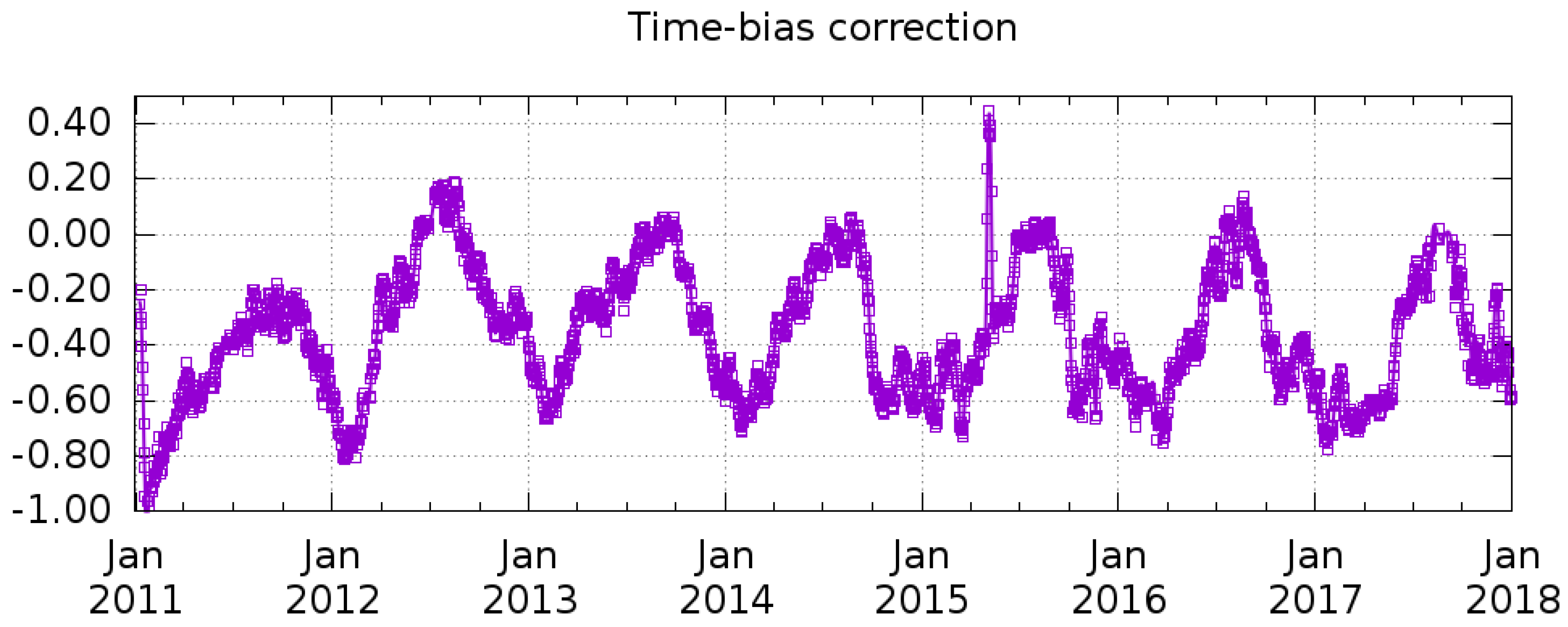
- Mitigation of the seasonal bias: An additional time-dependent bias correction is needed to mitigate the effect of seasonal and other time-dependent biases which affect the SMOS ([19]). In [23], the authors proposed subtracting the global mean of the SMOS SSS anomaly for each nine-day map. This assumption is appropriate for global SSS maps, as it implies that the total content of salt remains constant in time. However, the application of this hypothesis regionally, in particular at high latitudes, produces seasonal biases. In other words, there are net exchanges of salinity across region boundaries. In a recent study [25], a multivariate analysis is used to characterize and mitigate the time-dependent bias in the SMOS SSS maps in the Mediterranean Sea. In this work, we include a simpler time-dependent bias correction:
- We consider the Argo SSS available for the same nine-day period used in the generation of the nine-day SMOS SSS maps.
- We compute the median of the differences between the collocated SMOS SSS fields and the Argo SSS.
- We subtract this median from each nine-day SMOS SSS map.
4. Quality Assessment of the SMOS SSS Data
4.1. Comparison with TARA SSS: Impact Analysis of the SSS Annual Reference
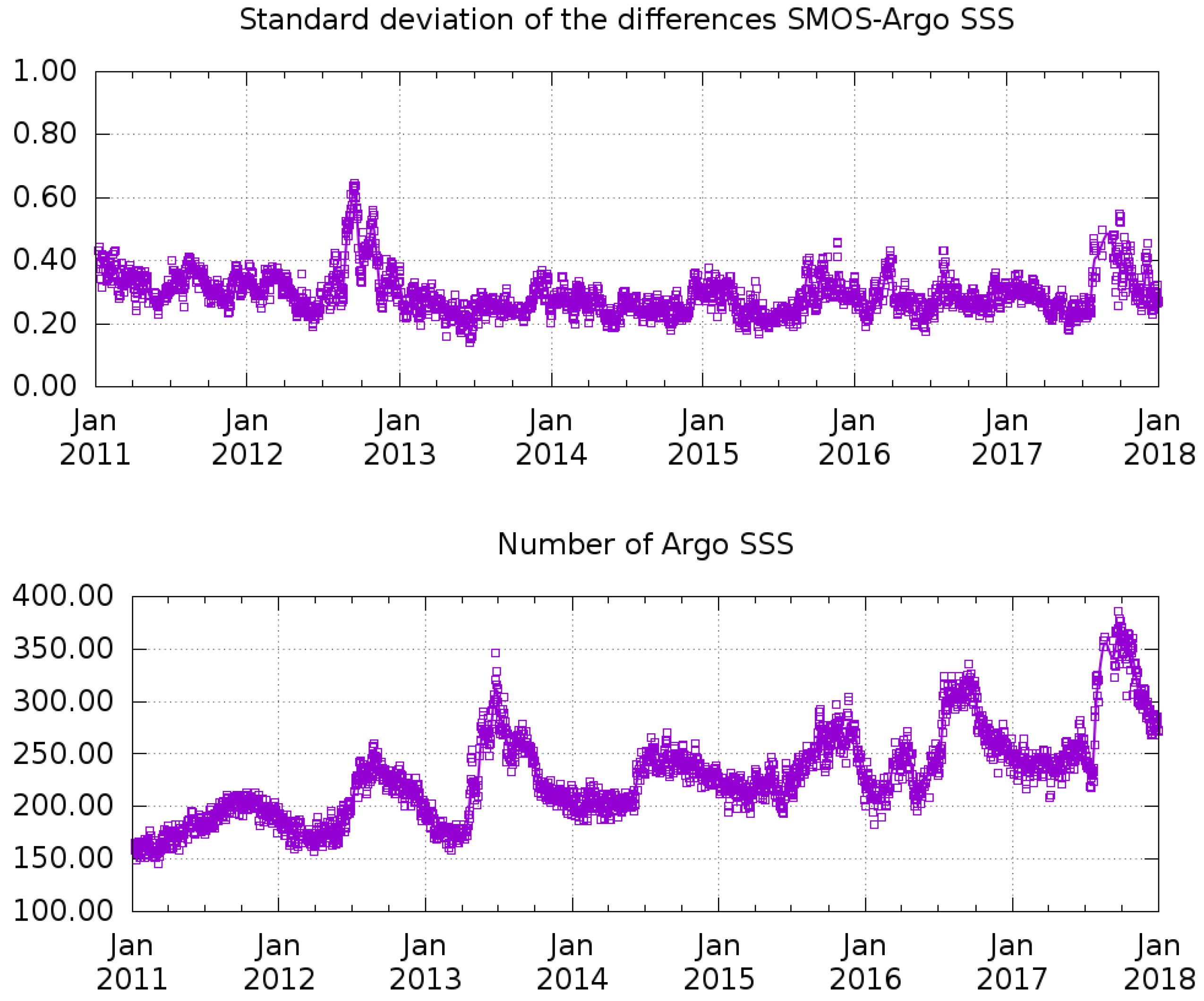
4.2. Comparison with Argo SSS
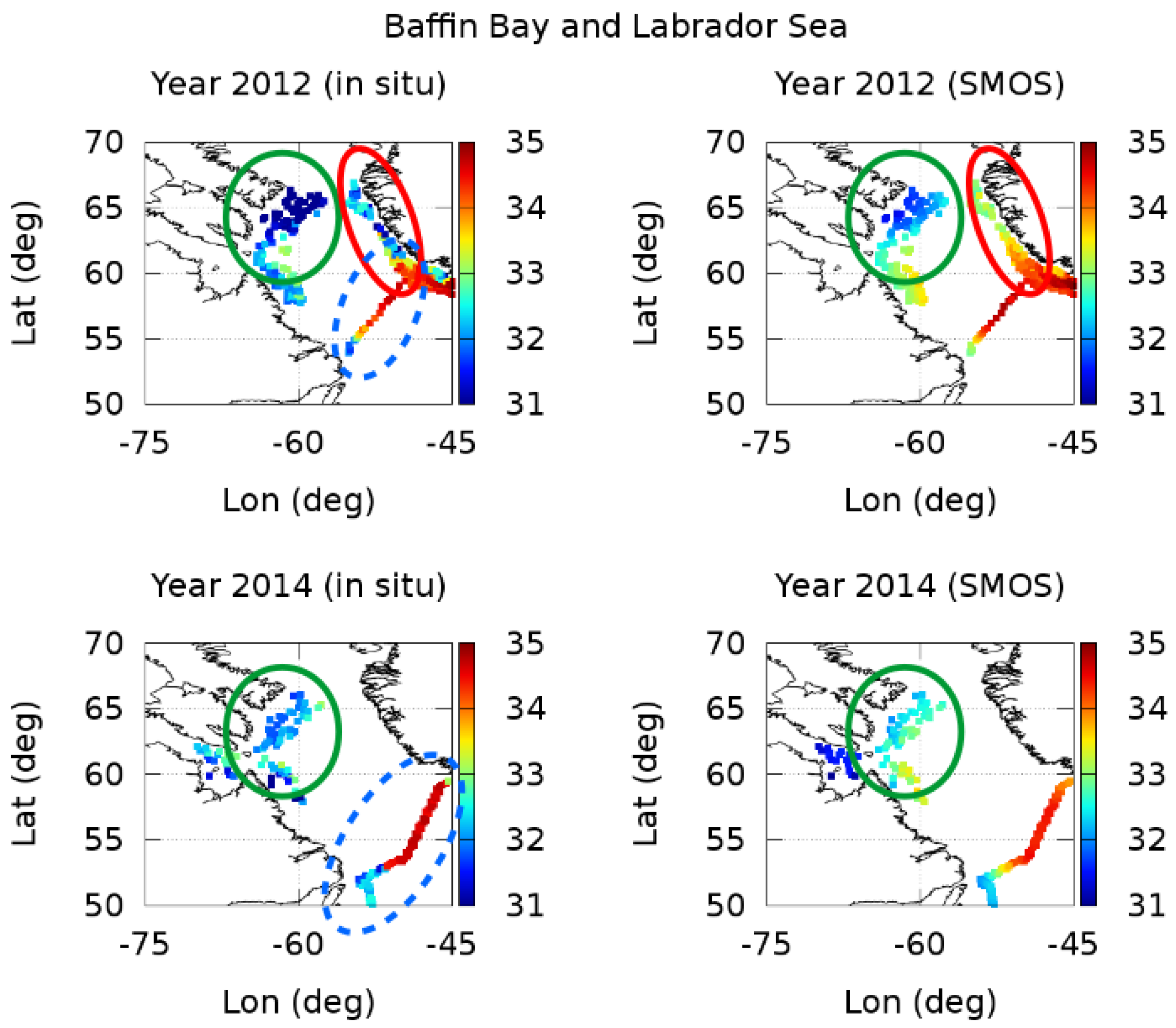
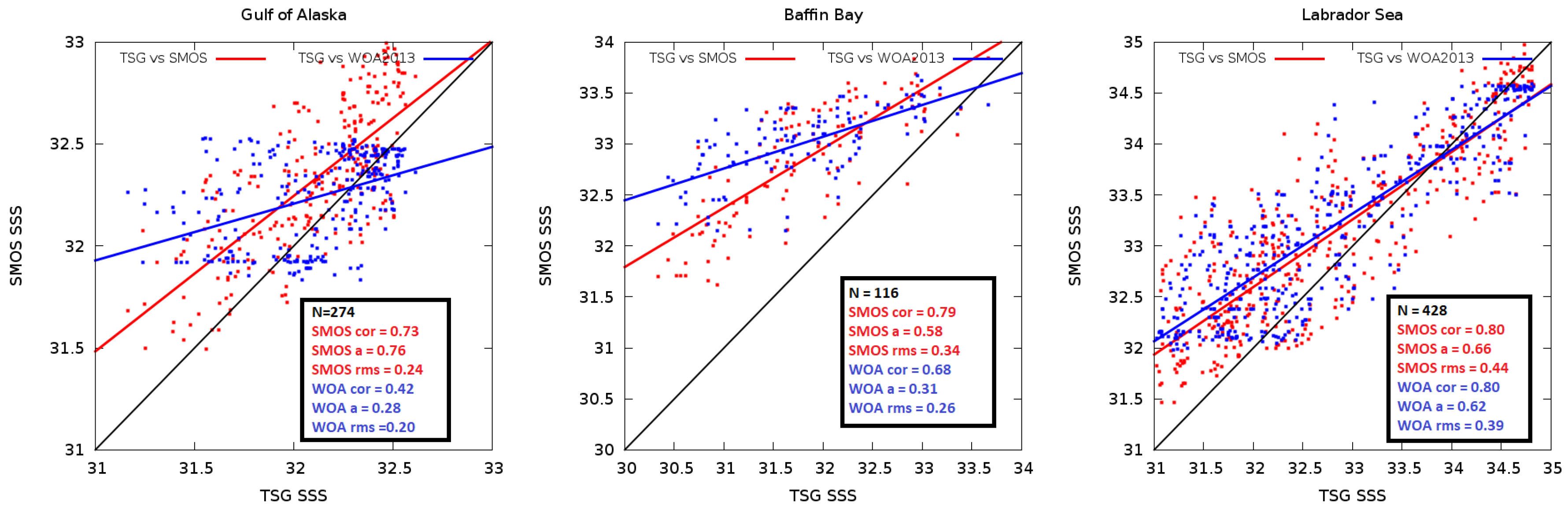
4.3. Comparison with TSG Data from Copernicus
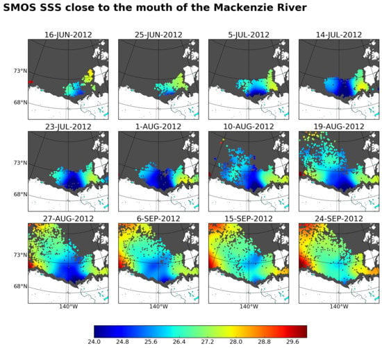
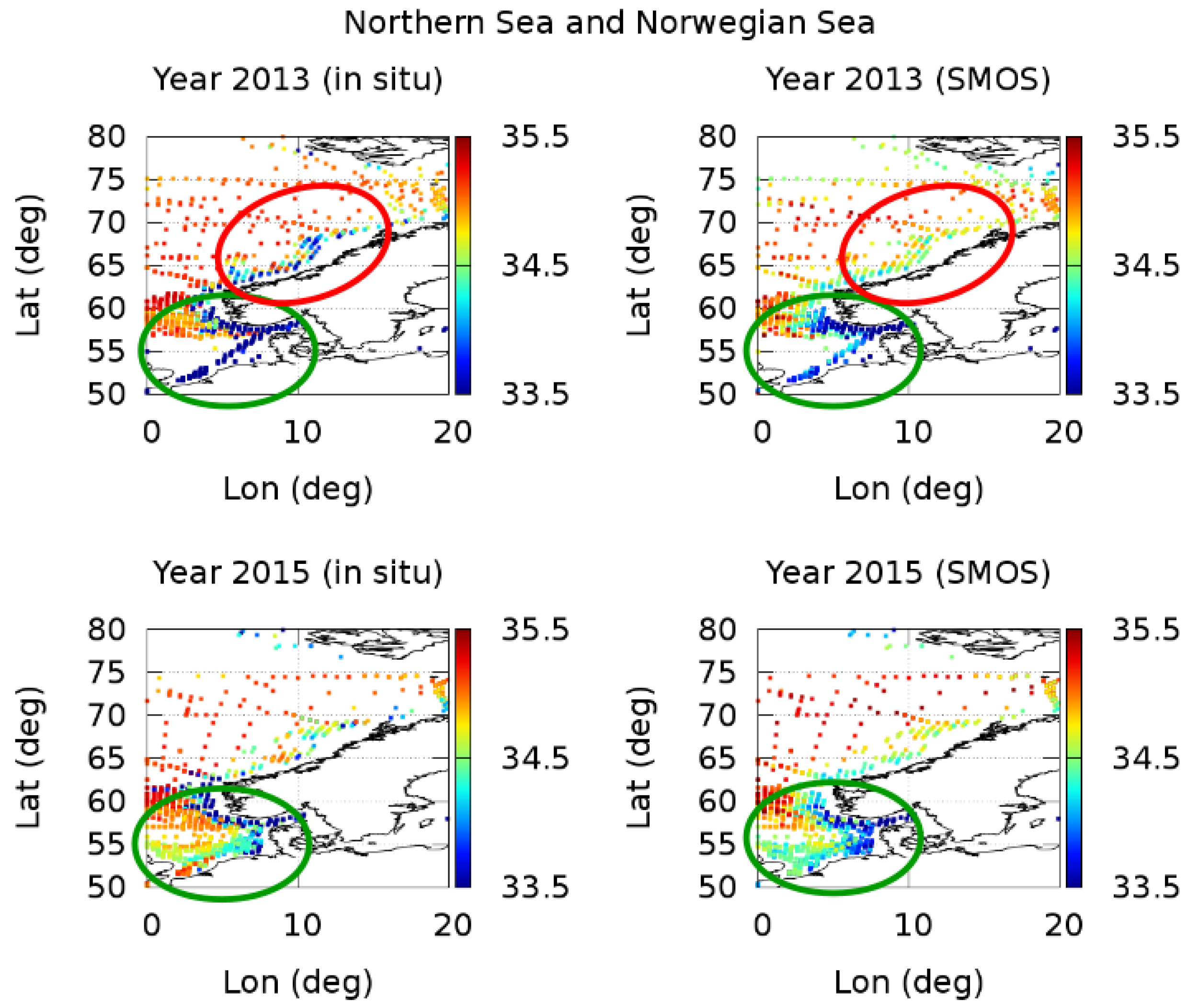
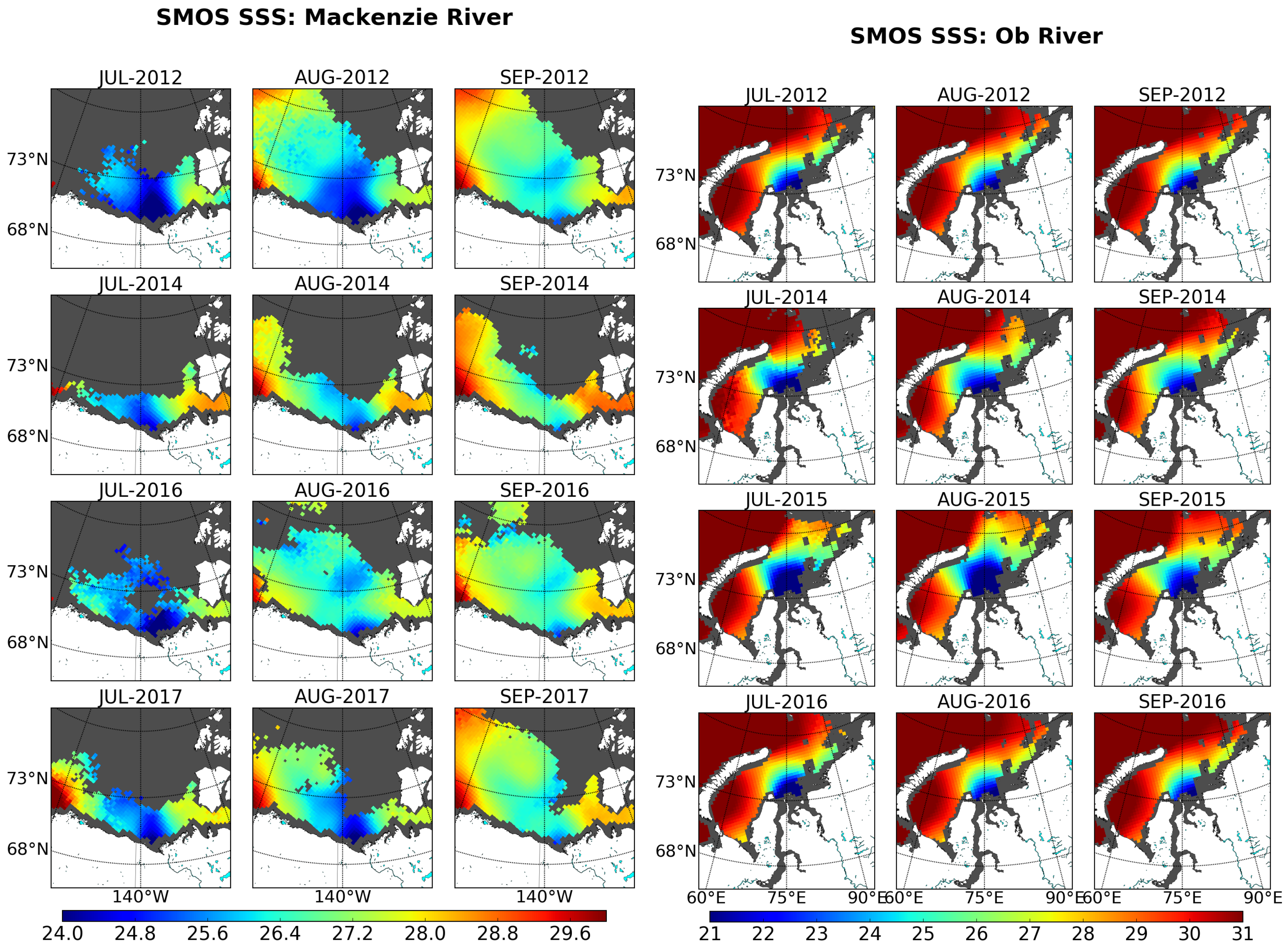
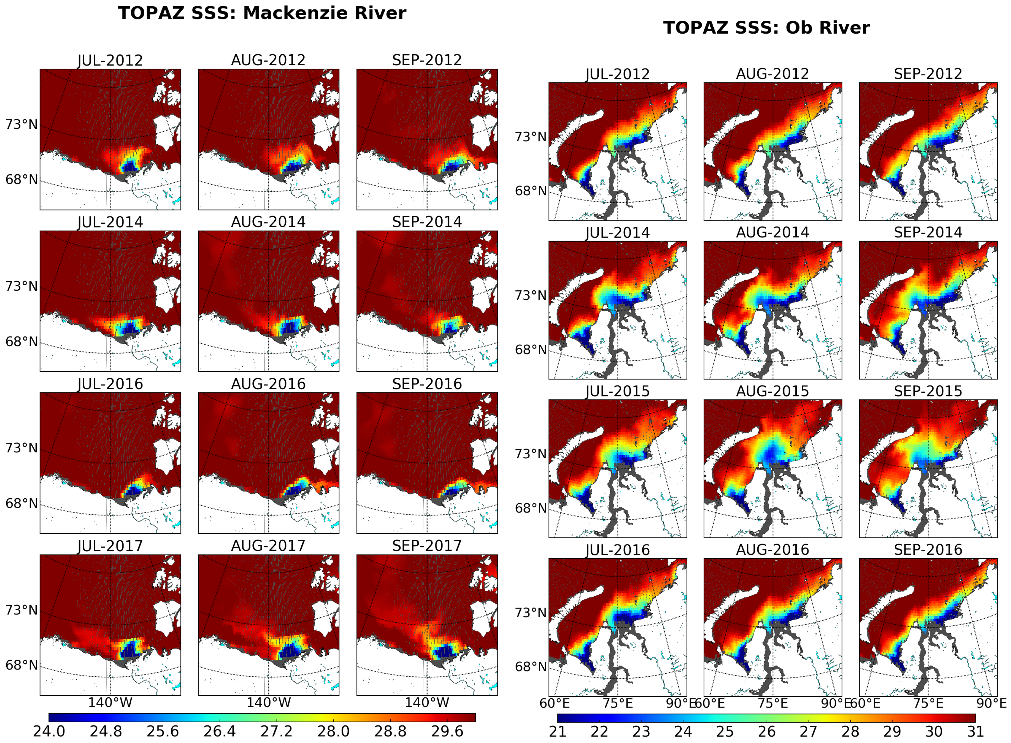
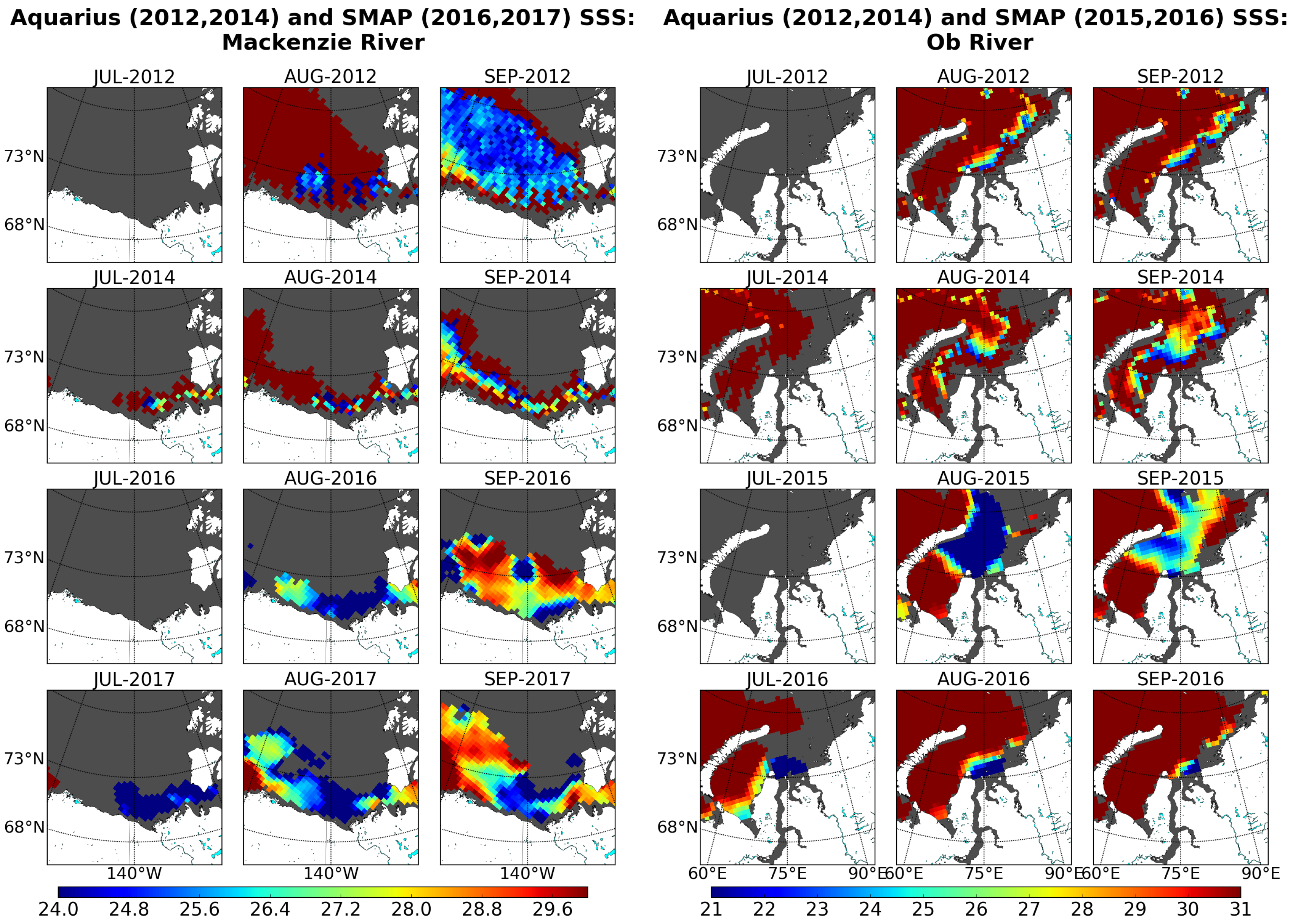
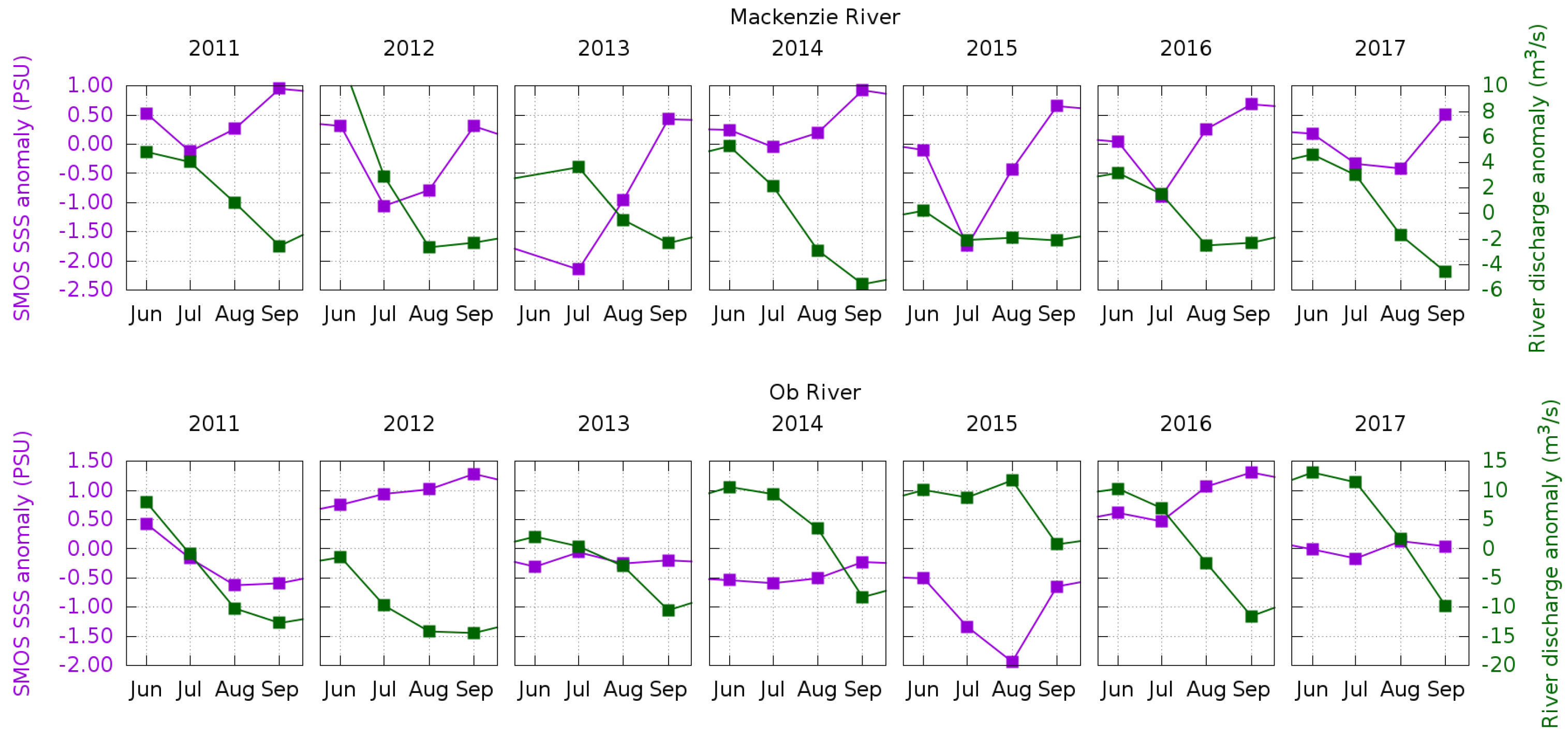
5. Sea Surface Salinity Variability Observed by SMOS at the Mouth of the Main Arctic Rivers
6. Conclusions
Author Contributions
Funding
Acknowledgments
Conflicts of Interest
References
- Serreze, M.C.; Holland, M.M.; Stroeve, J. Perspectives on theArctic’s shrinking sea-ice cover. Science 2007, 315, 1533–1536. [Google Scholar] [CrossRef] [PubMed]
- Haas, C.; Pfaffling, A.; Hendricks, S.; Rabenstein, L.; Etienne, J.L.; Rigor, I. Reduced ice thickness in Arctic transpolar drift favors rapid ice retreat. Geophys. Res. Lett. 2008, 35. [Google Scholar] [CrossRef]
- Comiso, J.C. Large Decadal Decline of the Arctic Multiyear Ice Cover. J. Clim. 2012, 25, 1176–1193. [Google Scholar] [CrossRef]
- Haine, T.; Curry, B.; Gerdes, R.; Hansen, E.; Karcher, M.; Lee, C.; Rudels, B.; Spreen, G.; de Steur, L.; Stewart, K.D.; et al. Arctic freshwater export: Status, mechanisms, and prospects. Glob. Planet. Chang. 2015, 125, 13–35. [Google Scholar] [CrossRef]
- Zhang, J.; Steele, M.; Runciman, K.; Dewey, S.; Morison, J.; Lee, C.; Rainville, L.; Cole, S.; Krishfield, R.; Timmermans, M.L.; et al. The Beaufort Gyre intensification and stabilization: A model-observation synthesis. J. Geophys. Res. Oceans 2016. [Google Scholar] [CrossRef]
- Rabe, B.; Karcher, M.; Kauker, F.; Schauer, U.; Toole, J.M.; Krishfield, R.A.; Pisarev, S.; Kikuchi, T.; Su, J. Arctic Ocean basin liquid freshwater storage trend 1992–2012. Geophys. Res. Lett. 2014, 41, 961–968. [Google Scholar] [CrossRef]
- Peterson, B.; Holmes, R.; McClelland, J.; Vörösmarty, C.; Lammers, R.; Shiklomanov, A.; Shiklomanov, I.; Rahmstorf, S. Increasing river discharge to the Arctic Ocean. Science 2002, 298, 2171–2173. [Google Scholar] [CrossRef] [PubMed]
- Mulligan, R.P.; Perrie, W.; Solomon, S. Dynamics of the Mackenzie River plume on the inner Beaufort shelf during an open water period in summer. Estuar. Coast. Shelf Sci. 2010, 89, 214–220. [Google Scholar] [CrossRef]
- Jeffries, M.; Richter-Menge, J.; Overland, J.E. Arctic Report Card 2015. Technical Report, NOAA Reports. Available online: https://www.arctic.noaa.gov/Report-Card (accessed on 8 November 2018).
- Font, J.; Camps, A.; Ballabrera-Poy, J. ‘Microwave Aperture Synthesis radiometry: Setting the Path for Sea Surface Salinity Measurements from Space’ in Remote Sensing of European Seas; Springer: Berlin, Germany, 2008; ISBN 978-1-4020-6771-6. [Google Scholar]
- Mecklenburg, S.; Wright, N.; Bouzina, C.; Delwart, S. Getting down to business—SMOS operations and products. ESA Bull. 2009, 137, 25–30. [Google Scholar]
- Kerr, Y.; Waldteufel, P.; Wigneron, J.; Delwart, S.; Cabot, F.; Boutin, J.; Escorihuela, M.; Font, J.; Reul, N.; Gruhier, C.; et al. The SMOS mission: New tool for monitoring key elements of the global water cycle. Proc. IEEE 2010, 98, 666–687. [Google Scholar] [CrossRef]
- Le Vine, D.; Lagerloef, G.; Colomb, F.; Yeh, S.; Pellerano, F. Aquarius: an instrument to monitor sea surface salinity from space. IEEE Trans. Geosci. Remote Sens. 2007, 45, 2040–2050. [Google Scholar] [CrossRef]
- Lagerloef, G.; Colomb, F.; LeVine, D.; Wentz, F.; Yueh, S.; Ruf, C.; Lilly, J.; Gunn, J.; Chao, Y.; de Charon, A.; et al. The Aquarius/Sac-D mission: designed to meet the salinity remote-sensing challenge. Oceanography 2008, 21, 68–81. [Google Scholar] [CrossRef]
- Entekhabi, D.; Njoku, E.; O’Neill, P.; Kellogg, K.; Crow, W.; Edelstein, W.; Entin, J.; Goodman, S.; Jackson, T.; Johnson, J.; et al. The Soil Moisture Active Passive (SMAP) mission. Proc. IEEE 2010, 98, 704–716. [Google Scholar] [CrossRef]
- Zine, S.; Boutin, J.; Font, J.; Reul, N.; Waldteufel, P.; Gabarro, C.; Tenerelli, J.; Petitcolin, F.; Vergely, J.; Talone, M.; et al. Overview of the SMOS Sea Surface Salinity Prototype Processor. IEEE Trans. Geosci. Remote Sens. 2008, 46, 621–645. [Google Scholar] [CrossRef]
- Swift, C.; McIntosh, R. Considerations for Microwave Remote Sensing of Ocean-Surface salinity. IEEE Trans. Geosci. Electron. 1983, GE-21, 480–491. [Google Scholar] [CrossRef]
- Yueh, S.; West, R.; Wilson, W.; Li, F.; Nghiem, S.; Rahmat-Samii, Y. Error Sources and Feasibility for Microwave Remote Sensing of Ocean Surface Salinity. IEEE Trans. Geosci. Remote Sens. 2001, 39, 1049–1059. [Google Scholar] [CrossRef]
- Martín-Neira, M.; Oliva, R.; Corbella, I.; Torres, F.; Duffo, N.; Duran, I.; Kainulainen, J.; Closa, A.; Zurita, A.; Cabot, F.; et al. SMOS Instrument performance and calibration after six years in orbit. Remote Sens. Environ. 2016, 180, 19–39. [Google Scholar] [CrossRef]
- Köhler, J.; Sena Martins, M.; Serra, N.; Stammer, D. Quality assessment of spaceborne sea surface salinity observations over the northern North Atlantic. J. Geophys. Res. Oceans 2015, 120, 94–112. [Google Scholar] [CrossRef]
- Matsuoka, A.; Babin, M.; Devred, E. A new algorithm for discriminating water sources from space: A case study for the southern Beaufort Sea using MODIS ocean color and SMOS salinity data. Remote Sens. Environ. 2016, 184, 124–138. [Google Scholar] [CrossRef]
- Tang, W.; Yueh, S.; Yang, D.; Fore, A.; Hayashi, A.; Lee, T.; Fournier, S.; Holt, B. The Potential and Challenges of Using Soil Moisture Active Passive (SMAP) Sea Surface Salinity to Monitor Arctic Ocean Freshwater Changes. Remote Sens. 2018, 10. [Google Scholar] [CrossRef]
- Olmedo, E.; Martinez, J.; Turiel, A.; Ballabrera-Poy, J.; Portabella, M. Debiased non-Bayesian retrieval: A novel approach to SMOS Sea Surface Salinity. Remote Sens. Environ. 2017, 193, 103–126. [Google Scholar] [CrossRef]
- Isern-Fontanet, J.; Olmedo, E.; Turiel, A.; Ballabrera-Poy, J.; García–Ladona, E. Retrieval of eddy dynamics from SMOS sea surface salinity measurements in the Algerian Basin (Mediterranean Sea). Geophys. Res. Lett. 2016, 43, 6427–6434. [Google Scholar] [CrossRef]
- Olmedo, E.; Taupier-Letage, I.; Turiel, A.; Alvera-Azcárate, A. Improving SMOS Sea Surface Salinity in the Western Mediterranean Sea through Multivariate and Multifractal Analysis. Remote Sens. 2018, 10. [Google Scholar] [CrossRef]
- Garcia-Eidell, C.; Comiso, J.; Dinnat, E.; Brucker, L. Satellite observed salinity distributions at high latitudes in the Northern Hemisphere: A comparison of four products. J. Geophys. Res. Ocean 2017, 122, 7717–7736. [Google Scholar] [CrossRef]
- Argo. Argo float data and metadata from Global Data Assembly Centre (Argo GDAC). SEANOE 2000. [Google Scholar] [CrossRef]
- Reverdin, G.; Le Goff, H.; Tara Oceans Consortium, Coordinators; Tara Oceans Expedition, Participants. Properties of seawater from a Sea-Bird TSG temperature and conductivity sensor mounted on the continuous surface water sampling system during campaign TARA_20090913Z of the Tara Oceans expedition 2009–2013. PANGAEA 2014. [Google Scholar] [CrossRef]
- Chassignet, E.P.; Hurlburt, H.E.; Metzger, E.J.; Smedstad, O.M.; Cummings, J.; Halliwell, G.R.; Bleck, R.; Baraille, R.; Wallcraft, A.; Lozano, C.; et al. Global Ocean Prediction with the HYbrid Coordinate Ocean Model (HYCOM). Oceanography 2009, 22, 64–75. [Google Scholar] [CrossRef]
- Sakov, P.; Counillon, F.; Bertino, L.; Lisæter, K.A.; Oke, P.R.; Korablev, A. TOPAZ4: An ocean-sea ice data assimilation system for the North Atlantic and Arctic. Ocean Sci. 2012, 8, 633–656. [Google Scholar] [CrossRef]
- Korosov, A.; Counillon, F.; Johannessen, A. Monitoring the spreading of the Amazon freshwater plume by MODIS, SMOS, Aquarius and TOPAZ. J. Geophys. Res. Oceans 2015, 120, 268–283. [Google Scholar] [CrossRef]
- Brucker, L.; Dinnat, E.; Koenig, L. Aquarius L3 Weekly Polar-Gridded Sea Surface Salinity, Version 6; NASA National Snow and Ice Data Center Distributed Active Archive Center: Boulder, CO, USA, 2015. [Google Scholar] [CrossRef]
- Brodzik, M.J.; Billingsley, B.; Haran, T.; Raup, B.; Savoie, M.H. EASE-Grid 2.0: Incremental but Significant Improvements for Earth-Gridded Datasets. ISPRS Int. J. Geo-Inf. 2012, 1, 32–45. [Google Scholar] [CrossRef]
- Fore, A.G.; Yueh, S.H.; Tang, W.; Stiles, B.W.; Hayashi, A.K. Combined Active/Passive Retrievals of Ocean Vector Wind and Sea Surface Salinity With SMAP. IEEE Trans. Geosci. Remote Sens. 2016, 54, 7396–7404. [Google Scholar] [CrossRef]
- Tenerelli, J.; Reul, N.; Mouche, A.; Chapron, B. Earth-Viewing L-Band Radiometer Sensing of Sea Surface Scattered Celestial Sky Radiation—Part I: General Characteristics. IEEE Trans. Geosci. Remote Sens. 2008, 46, 659–674. [Google Scholar] [CrossRef]
- Reul, N.; Tenerelli, J.; Guimbard, S.; Collard, F.; Kerbaol, V.; Skou, N.; Cardellach, E.; Tauriainen, S.; Bouzinac, C.; Wursteisen, P.; et al. Analysis of L-band radiometric measurements conducted over the North Sea during the CoSMOS-OS airborne campaign. In Proceedings of the IEEE International Geoscience and Remote Sensing Symposium (IGARSS2007), Barcelona, Spain, 23–27 July 2007. [Google Scholar]
- Guimbard, S.; Gourrion, J.; Portabella, M.; Turiel, A.; Gabarro, C.; Font, J. SMOS Semi-Empirical Ocean Forward Model Adjustment. IEEE Trans. Geosci. Remote Sens. 2012, 50, 1676–1687. [Google Scholar] [CrossRef]
- Sabater, J.; De Rosnay, P. Tech Note—Parts 1/2/3: Operational Pre-processing Chain, Collocation Software Development and Offline Monitoring Suite; Technical Report; ECMWF: Reading, UK, 2010. [Google Scholar]
- Meissner, T.; Wentz, F. The complex dielectric constant of pure and sea water from microwave satellite observations. IEEE Trans. Geosci. Remote Sens. 2004, 42, 1836–1849. [Google Scholar] [CrossRef]
- Klein, L.; Swift, C. An Improved Model for the Dielectric Constant of Sea Water at Microwave Frequencies. IEEE Trans. Antennas Propag. 1977, AP-25, 104–111. [Google Scholar] [CrossRef]
- Dinnat, E.P.; Boutin, J.; Yin, X.; Vine, D.M.L. Inter-comparison of SMOS and Aquarius Sea Surface Salinity: Effects of the dielectric constant and vicarious calibration. In Proceedings of the 2014 13th Specialist Meeting on Microwave Radiometry and Remote Sensing of the Environment (MicroRad), Pasadena, CA, USA, 24–27 March 2014; pp. 55–60. [Google Scholar] [CrossRef]
- Brodzik, M.J.; Knowles, K.W. EASE-Grid: A Versatile Set of Equal-Area Projections and Grids. In Discrete Global Grids; National Center for Geographic Information & Analysis: Santa Barbara, CA, USA, 2002. [Google Scholar]
- Gabarro, C.; Portabella, M.; Talone, M.; Font, J. Toward an Optimal SMOS Ocean Salinity Inversion Algorithm. IEEE Geosci. Remote Sens. Lett. 2009, 6, 509–513. [Google Scholar] [CrossRef]
- Tenerelli, J.; Reul, N. Analysis of L1PP Calibration Approach Impacts in SMOS Tbs and 3-Days SSS Retrievals over the Pacific Using an Alternative Ocean Target Transformation Applied to L1OP Data; Technical Report; IFREMER/CLS: Paris, France, 2010. [Google Scholar]
- Zweng, M.; Reagan, J.; Antonov, J.; Locarnini, R.; Mishonov, A.; Boyer, T.; Garcia, H.; Baranova, O.; Johnson, D.; Seidov, D.; et al. World Ocean Atlas 2013, Volume 2: Salinity; A. Mishonov Technical, Levitus, Eds.; NOAA Atlas NESDIS 74; NOAA: Washington, DC, USA, 2013; p. 39.
- Steele, M.; Morley, R.; Ermold, W. PHC: A global ocean hydrography with a high-quality Arctic Ocean. J. Clim. 2001, 9, 2079–2087. [Google Scholar] [CrossRef]
- Nurser, A.; Bacon, S. The Rossby radius in the Arctic Ocean. Ocean Sci. 2014, 10, 967–975. [Google Scholar] [CrossRef]
- González-Gambau, V.; Turiel, A.; Olmedo, E.; Martínez, J.; Corbella, I.; Camps, A. Nodal Sampling: A New Image Reconstruction Algorithm for SMOS. IEEE Trans. Geosci. Remote Sens. 2016, 54, 2314–2328. [Google Scholar] [CrossRef]
- González-Gambau, V.; Olmedo, E.; Turiel, A.; Martínez, J.; Ballabrera-Poy, J.; Portabella, M.; Piles, M. Enhancing SMOS brightness temperatures over the ocean using the nodal sampling image reconstruction technique. Remote Sens. Environ. 2016, 180, 202–220. [Google Scholar] [CrossRef]
- González-Gambau, V.; Olmedo, E.; Martínez, J.; Turiel, A.; Duran, I. Improvements on Calibration and Image Reconstruction of SMOS for Salinity Retrievals in Coastal Regions. IEEE J. Sel. Top. Appl. Earth Obs. Remote Sens. 2017, 10, 3064–3078. [Google Scholar] [CrossRef]
- Boutin, J.; Chao, Y.; Asher, W.E.; Delcroix, T.; Drucker, R.; Drushka, K.; Kolodziejczyk, N.; Lee, T.; Reul, N.; Reverdin, G.; et al. Satellite and In Situ Salinity: Understanding Near-Surface Stratification and Subfootprint Variability. Bull. Am. Meteorol. Soc. 2016, 97, 1391–1407. [Google Scholar] [CrossRef]
- Comiso, J.C.; Meier, W.N.; Gersten, R. Variability and trends in the Arctic Sea ice cover: Results from different techniques. J. Geophys. Res. Oceans 2017, 122, 6883–6900. [Google Scholar] [CrossRef]


| Arctic Region | SMOS woa | WOA | SMOS phc | PHC | ||||||||
|---|---|---|---|---|---|---|---|---|---|---|---|---|
| Mean | Std | RMS | Mean | Std | RMS | Mean | Std | RMS | Mean | Std | RMS | |
| Norwegian sea | 0.11 | 0.15 | 0.18 | −0.06 | 0.19 | 0.20 | −0.18 | 0.19 | 0.26 | −0.13 | 0.24 | 0.28 |
| Baffin Bay | 0.16 | 0.46 | 0.49 | 0.04 | 0.49 | 0.50 | 0.29 | 0.55 | 0.63 | 0.17 | 0.51 | 0.54 |
| Chukchi region | 2.16 | 2.18 | 3.07 | 2.74 | 2.26 | 3.55 | 3.46 | 2.79 | 4.44 | 4.02 | 2.87 | 4.94 |
| Barents sea | −1.35 | 1.37 | 1.93 | −1.22 | 1.58 | 2.00 | −0.86 | 1.24 | 1.51 | −0.73 | 1.46 | 1.64 |
| Laptev sea | 1.37 | 3.48 | 3.74 | 1.78 | 3.37 | 3.81 | 1.46 | 4.16 | 4.41 | 1.87 | 4.02 | 4.43 |
| Siberian region | −3.20 | 2.50 | 4.06 | −2.88 | 2.93 | 4.11 | −1.54 | 2.39 | 2.84 | −1.21 | 2.72 | 2.98 |
| Norwegian Sea | Baffin Bay | Chukchi Region | Barents Sea | Laptev Sea | Siberian Region | |
|---|---|---|---|---|---|---|
| SMOS woa | 0.73 | 0.51 | 0.91 | 0.88 | 0.68 | 0.80 |
| SMOS phc | 0.56 | −0.20 | 0.86 | 0.91 | 0.28 | 0.81 |
| Region | Latitude Range | Longitude Range | SMOS-TSG | SMOS-ARGO | ||||
|---|---|---|---|---|---|---|---|---|
| Meas | Mean | Std | Meas | Mean | Std | |||
| Denmark Strait | 60N–65N | 40W–25W | 2322 | 0.22 | 0.28 | 25,153 | 0.02 | 0.21 |
| North Atlantic | 50N–60N | 50W–20W | 8028 | 0.19 | 0.45 | 102,575 | 0.01 | 0.35 |
| Norwegian Sea | 60N–70N | 10W–5E | 4587 | 0.02 | 0.67 | 33,841 | −0.05 | 0.31 |
| Northern Sea | 55N–60N | 0E–5E | 53,366 | 0.16 | 0.99 | 0 | - | - |
| Gulf of Alaska | 55N–60N | 175W–125W | 604 | 0.26 | 0.72 | 14,841 | 0.09 | 0.27 |
| Chuckchi Sea | 70N–75N | 170W–145W | 315 | 0.01 | 1.42 | 1751 | −0.99 | 0.37 |
| Labrador Sea | 55N–60N | 55W–45W | 737 | 0.14 | 0.71 | 33,711 | −0.07 | 0.29 |
| Baffin Bay | 60N–65N | 65W–55W | 278 | 0.89 | 0.62 | 5919 | −0.02 | 0.41 |
© 2018 by the authors. Licensee MDPI, Basel, Switzerland. This article is an open access article distributed under the terms and conditions of the Creative Commons Attribution (CC BY) license (http://creativecommons.org/licenses/by/4.0/).
Share and Cite
Olmedo, E.; Gabarró, C.; González-Gambau, V.; Martínez, J.; Ballabrera-Poy, J.; Turiel, A.; Portabella, M.; Fournier, S.; Lee, T. Seven Years of SMOS Sea Surface Salinity at High Latitudes: Variability in Arctic and Sub-Arctic Regions. Remote Sens. 2018, 10, 1772. https://doi.org/10.3390/rs10111772
Olmedo E, Gabarró C, González-Gambau V, Martínez J, Ballabrera-Poy J, Turiel A, Portabella M, Fournier S, Lee T. Seven Years of SMOS Sea Surface Salinity at High Latitudes: Variability in Arctic and Sub-Arctic Regions. Remote Sensing. 2018; 10(11):1772. https://doi.org/10.3390/rs10111772
Chicago/Turabian StyleOlmedo, Estrella, Carolina Gabarró, Verónica González-Gambau, Justino Martínez, Joaquim Ballabrera-Poy, Antonio Turiel, Marcos Portabella, Severine Fournier, and Tong Lee. 2018. "Seven Years of SMOS Sea Surface Salinity at High Latitudes: Variability in Arctic and Sub-Arctic Regions" Remote Sensing 10, no. 11: 1772. https://doi.org/10.3390/rs10111772
APA StyleOlmedo, E., Gabarró, C., González-Gambau, V., Martínez, J., Ballabrera-Poy, J., Turiel, A., Portabella, M., Fournier, S., & Lee, T. (2018). Seven Years of SMOS Sea Surface Salinity at High Latitudes: Variability in Arctic and Sub-Arctic Regions. Remote Sensing, 10(11), 1772. https://doi.org/10.3390/rs10111772