Article

High-Throughput Phenotyping of Crop Water Use Efficiency via Multispectral Drone Imagery and a Daily Soil Water Balance Model

1
USDA-ARS, Arid-Land Agricultural Research Center, Maricopa, AZ 85138, USA
2
Maricopa Agricultural Center, University of Arizona, Maricopa, AZ 85138, USA
*
Author to whom correspondence should be addressed.
Remote Sens. 2018, 10(11), 1682; https://doi.org/10.3390/rs10111682
Submission received: 12 September 2018 / Revised: 19 October 2018 / Accepted: 22 October 2018 / Published: 25 October 2018

Abstract

:
Improvement of crop water use efficiency (CWUE), defined as crop yield per volume of water used, is an important goal for both crop management and breeding. While many technologies have been developed for measuring crop water use in crop management studies, rarely have these techniques been applied at the scale of breeding plots. The objective was to develop a high-throughput methodology for quantifying water use in a cotton breeding trial at Maricopa, AZ, USA in 2016 and 2017, using evapotranspiration (ET) measurements from a co-located irrigation management trial to evaluate the approach. Approximately weekly overflights with an unmanned aerial system provided multispectral imagery from which plot-level fractional vegetation cover ( f c ) was computed. The f c data were used to drive a daily ET-based soil water balance model for seasonal crop water use quantification. A mixed model statistical analysis demonstrated that differences in ET and CWUE could be discriminated among eight cotton varieties ( p < 0 . 05 ), which were sown at two planting dates and managed with four irrigation levels. The results permitted breeders to identify cotton varieties with more favorable water use characteristics and higher CWUE, indicating that the methodology could become a useful tool for breeding selection.

Graphical Abstract

1. Introduction

Drought stress arising from water deficit is a leading cause of crop production losses worldwide. Specific regions of the world are also projected to experience increases in the frequency and severity of future drought events due to effects of climate change on precipitation patterns [1,2]. To maintain productivity and security of food, fiber, and other agricultural products, increasing crop water use efficiency (CWUE), defined as the ratio of crop yield and water consumption volume, is an important goal to ameliorate impacts of future drought. Increases in CWUE can result both from improvements in agronomic management practices [3] and by developing improved crop cultivars that yield highly under water deficit conditions [4]. Although these pathways are often pursued independently within disciplinary boundaries, the most comprehensive solutions towards CWUE improvement will be achieved through multidisciplinary efforts.
Adoption of information technologies for problem solving in the agricultural sciences has been an especially pervasive occurrence in recent years. For example, precision irrigation, where water applications are tuned based on the spatial and temporal crop need, is a primary technology for improving CWUE in crop production settings [5,6]. Other agronomic solutions involve improved fertility management, optimizing sowing dates, using cover crops or mulches, and choosing alternative crops or crop rotations [3]. In the plant sciences, high-throughput plant phenomics, which involves deployment of crop sensing systems for rapid phenotyping of breeding populations, has potential to guide crop improvement efforts toward cultivars with increased tolerance to drought stress [4,7,8]. Information technologies in the form of sensors, imagers, data loggers, sensor deployment vehicles, geographic information systems, geostatistical methods, data management approaches, and engineering control systems are central to the success of these technical solutions to improving CWUE. However, further efforts are needed to solidify the role of information technology for practical advancement towards this goal.
Remote sensing has been used to estimate crop evapotranspiration (ET) and predict drought stress at multiple scales [9,10,11,12,13]. For example, Yebra et al. [14] combined vegetation metrics derived from the MODerate resolution Imaging Spectroradiometer (MODIS) satellite with the Penman-Monteith equation to estimate ET for evergreen and deciduous broadleaf forests. At the agricultural field scale, Colaizzi et al. [15] installed infrared thermometers on an overhead sprinkler irrigation machine to estimate daily ET. They proposed that the approach could improve CWUE through better irrigation scheduling. In addition, Hunsaker et al. [16] used multispectral cameras aboard a manned helicopter to map the normalized difference vegetation index (NDVI) of a cotton (Gossypium hirsutum L.) field, estimated basal crop coefficients from NDVI, and scheduled irrigation using an ET-based soil water balance model [17]. Results for one growing season showed that the recommendations from the scheduling model led to increased CWUE when NDVI was used to estimate basal crop coefficients. Additional field testing is needed to further realize CWUE improvements using remote sensing to guide irrigation management decisions.
Leveraging the technology previously developed for precision agriculture applications, remote and proximal sensing has recently become a highly popular tool for field-based plant phenotyping, particularly by integrating imaging equipment with unmanned aerial systems (i.e., drones) to obtain very high resolution imagery of plant breeding trials. For example, Zaman-Allah et al. [18] related nitrogen stress, senescence, and yield for ten maize (Zea mays L.) hybrids to NDVI from multispectral images collected with a drone. In addition, Sankaran et al. [19] used a multispectral camera with a drone to estimate seedling emergence and stand density for more than 100 winter wheat (Triticum aestivum L.) varieties in Washington State. Condorelli et al. [20] measured NDVI with a drone-based multispectral camera over 248 durum wheat (Triticum durum L.) lines at different growth stages and water regimes. A subsequent genome-wide association study (GWAS) identified 22 single quantitative trait loci (QTL) for NDVI, particularly as related to terminal drought stress. Although many important advancements have been made, moving remote sensing data analyses beyond the NDVI will enhance the quantification of useful phenotypes.
Few studies, if any, have aimed to directly phenotype crop water use or CWUE for purposes of breeding or genomic analysis. Rather, the focus has been to estimate related plant traits, such as spectral indices that correlate with plant water status, under both well-watered and water-limited conditions [21,22,23,24]. A key difference is that plant water status describes the plant state at a singular time point, whereas crop water use is a process that occurs over time. For this reason, efforts to integrate process-based simulation models with spectral measurements of plant states may provide phenotypes that better express the process-based nature of plant growth and water consumption [25]. Although the integration of remote sensing data with models of radiation transfer, crop growth, and soil water balance has been widely studied for regional and field-scale mapping of crop water use, such techniques have not been applied for field-based, high-throughput plant phenomics.
The main goal of this study was to develop a methodology for phenotyping crop water use and CWUE in a cotton breeding trial, using ET estimates from a co-located irrigation management study to evaluate the approach. It attempts to merge efforts from the ET remote sensing community with efforts in the plant science community in a multidisciplinary effort toward CWUE improvement. Specific objectives were to (1) estimate fractional vegetation cover ( f c ) from multispectral images collected over the cotton field trials with a drone, (2) use plot-level f c to derive crop water use calculations from an ET-based daily soil water balance model, and (3) identify cotton cultivars with favorable yield, fiber quality and water use efficiency across treatments and growing seasons.

2. Materials and Methods

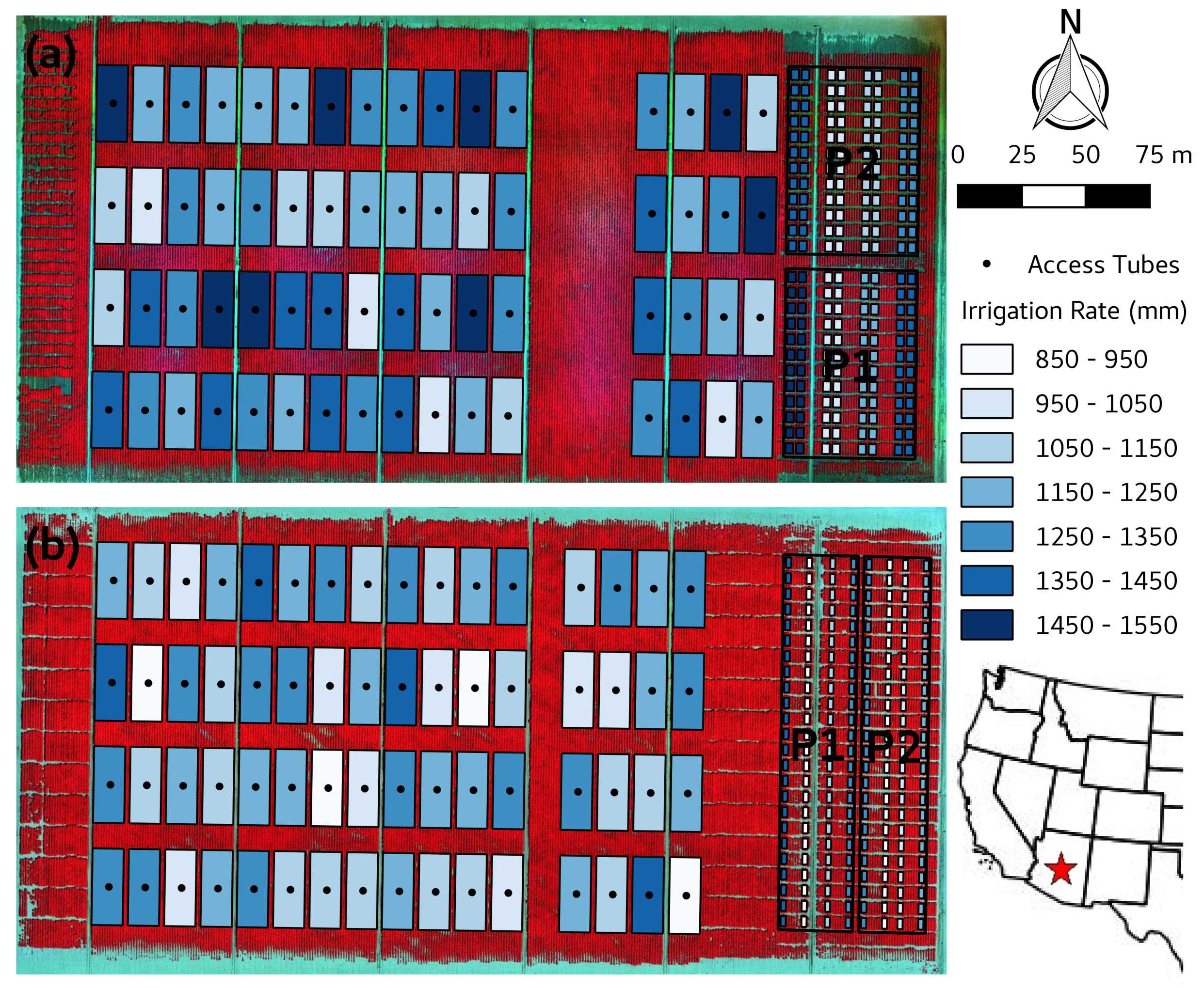
2.1. Field Experiments

Cotton field experiments were conducted at the University of Arizona’s Maricopa Agricultural Center (MAC) near Maricopa, AZ (33.079 N, 111.977 W, 360 m above sea level) during the 2016 and 2017 growing seasons (Figure 1). The environment in central Arizona is arid and hot, with maximum daily air temperatures regularly exceeding 38 C in July and August. Growing season precipitation from April through September amounted to 42 and 51 mm in 2016 and 2017, respectively. In comparison, short crop reference ET during the same period was 1364 and 1404 mm in 2016 and 2017, respectively. Thus, cotton production required irrigation to meet evaporative demand.
Soil variability at the 6-ha field site was characterized via a multi-year soil sampling effort at 160 locations (not shown). A tractor-mounted soil sampler (model 25-TS, Giddings Machine Co., Windsor, CO, USA) was used to collect cylindrical soil samples (0.04-m diameter × 0.4-m depth) at five incremental soil profile depths centered at 0.2, 0.6, 1.0, 1.4 and 1.8 m. Soil texture analysis was conducted in the laboratory using the hydrometer method of Gee and Bauder [26], and the soil water holding limits of each sample was computed from texture data using the Rosetta pedotransfer functions [27]. For ET estimation purposes (discussed below), ordinary kriging was used to spatially interpolate soil water limits at the central location of each field plot (Figure 1). Geostatistics were conducted using the “geoR” package within the R Project for Statistical Computing software. Primarily, soil texture at the field site was sandy loam and sandy clay loam with drained upper limits between 0.16 and 0.22 cm 3 cm - 3 and lower limits between 0.08 and 0.11 cm 3 cm - 3 .
Data from two field experiments (Experiment #1 and Experiment #2), each with a unique experimental design and purpose, were used to complete the objectives of this study. The two field experiments were established on adjacent land areas (Figure 1), both receiving irrigation from the same overhead, lateral-move sprinkler irrigation system (Zimmatic, Lindsay Corporation, Omaha, NE, USA). Advanced technology on the irrigation machine permitted the application of variable irrigation rates based on georeferenced irrigation maps uploaded to the machine’s control panel. The variable-rate irrigation system permitted unique control of irrigation rates from individual drop hoses, which were spaced 1.0 m apart and located at the center of each interrow area. Nozzles were positioned to emit water less than 1.0 m above the soil surface. For uniform soil wetting prior to cotton emergence, spray pads giving a spray diameter of approximately 5.0 m were used. After emergence, the pads were changed to a “bubbler” style, which emitted large droplets with a 0.3-m spray diameter at the center of each interrow area. In addition to reducing water loss to evaporation, the bubbler pads increased the spatial accuracy of irrigation applications relative to the intended application areas delineated in the georeferenced irrigation maps. Spatial application error with the variable-rate irrigation machine was estimated to be less than 2.0 m. The overhead irrigation system with variable-rate capability permitted both field experiments to incorporate multiple irrigation rates as a primary treatment.
Experiment #1 tested cotton yield and water use responses to variable irrigation rate and timing for one commercial cotton variety (Deltapine 1549 B2XF, Monsanto Company, St. Louis, MO, USA). Treatment plots were relatively large (12.2 m (12 cotton rows) × 30.0 m) and required a majority of the field area (Figure 1). The experimental design included four replications of sixteen irrigation management treatments (64 plots), which involved all the possible combinations of four irrigation rates applied during two distinct periods of the growing season. The four irrigation rates were 60%, 80%, 100%, and 120% of the recommendation provided by an irrigation scheduling tool based on the CSM-CROPGRO-Cotton agroecosystem model [28]. The two irrigation periods were from first square to peak bloom (approximately the first of June through mid-July) and from peak bloom to 90% open boll (approximately mid-July through the first week of September). The various combinations of the four rates during the two times resulted in sixteen total irrigation treatments, which led to cotton grown under a variety of soil water status conditions. The entire field area was disked and planed prior to planting. Cotton was planted with a north-south row orientation on 25 April 2016 (day of year (DOY) 116) and 18 April 2017 (DOY 108).
Of highest relevance to the present study, Experiment #1 incorporated weekly soil water content measurements via a field-calibrated neutron moisture meter (model 503, Campbell Pacific Nuclear, Martinez, CA, USA). After crop emergence, steel access tubes were installed at the center of each treatment plot (Figure 1) using the tractor-mounted soil sampler. From mid-May to early October, the neutron moisture meter was deployed on a weekly basis (approximately 20 times per growing season) to measure soil water content from 0.1 to 1.9 m in 0.2-m incremental depths at each access tube. Soil water content data were used to estimate ET and deep seepage (DS) between successive measurement events using the soil water balance approach described by Hunsaker et al. [29]:
ET = i = 1 7 ( D i , 1 - D i , n - 1 ) + j = 1 n - 1 ( R j + I j ) - DS ,
DS = max ( 0 . 0 , i = 8 10 ( D i , 1 - D i , n - 1 ) ) ,
where ET is the total evapotranspiration and DS is the total deep seepage occurring from the beginning of a given measurement day (denoted as day j = 1 ) to the end of the day before the successive measurement date (denoted as j = n - 1 ), D i , 1 and D i , n - 1 are respectively the water depth measurements at soil depth increment i at the beginning of day 1 and at the end of day n - 1 , and R j and I j are respectively the precipitation and net irrigation depths received on day j. For the sake of practicality, soil water content measurements collected on the morning of day n were used to approximate soil water content at the end of day n - 1 . Deep seepage was not permitted to be negative, meaning upflux from below the neutron access tube was considered negligible. The seasonal ET estimates from neutron moisture meter data provided important verification that the ET estimation methodology (discussed below) provided reasonably accurate results.
Experiment #2 was a breeding trial that tested the responses of eight cotton cultivars (Table 1) to two planting dates and four irrigation rates (Figure 1). The experimental design was a randomized complete block design with planting date as the block and irrigation rate treatments nested within the blocks. Each cultivar was replicated three times for each irrigation treatment, totaling 96 plots per block. The first planting date treatment was sown on 26 April 2016 (DOY 117) and 19 April 2017 (DOY 109), and the second planting date treatment was sown on 18 May 2016 (DOY 139) and 10 May 2017 (DOY 130). The four irrigation rates were 60%, 80%, 100%, and 120% of the recommendation provided by a simulation tool for irrigation scheduling [28] and were administered consistently from first square (early June) to 90% open boll (early September). Irrigation rates were administered uniformly within spatial areas containing 24 treatment plots (8 cultivars × 3 replications). Buffer areas with width of 6.0 m (six cotton rows) and planted to a single commercial cotton variety were incorporated centrally along the boundaries of irrigation treatments to prevent spatial error in the variable-rate irrigation application from affecting cultivar treatments. In 2016, the plot dimensions for cultivar treatments were 3.0 m (three cotton rows) × 4.6 m with a 1.5 m buffer area between plots. In 2017, the plot size was reduced to 2.0 m (two cotton rows) × 4.6 m, and the buffer area between plots remained 1.5 m. Due to the relatively small size and large number of treatment plots (i.e., 192 per growing season), plot-level ET estimation via neutron moisture meter measurements and other common ET measurement methodologies was impractical. Thus, this study aimed to estimate ET by integrating plot-specific remote sensing data and an ET-based soil water balance model with site-specific soil parameterization, providing an approach for high-throughput phenotyping of cotton water use in this breeding trial.
The cotton breeding trial was machine harvested with a two-row picker on 1 November 2016 (DOY 306) and 8 November 2017 (DOY 312). Samples from each plot were bagged and weighed separately in the field. Prior to the harvest date, 25 mature bolls were sampled from each plot and ginned on a small research-scale cotton gin. Harvest weight, fiber turnout percentage, and plot area were used to compute cotton fiber yield (kg ha - 1 ) for each plot. Additionally, cotton fiber from the 25 mature boll samples was sent to Cotton Incorporated (Cary, NC, USA) for analysis of fiber quality via High Volume Instrument (HVI) methods.

2.2. Multispectral Imaging

Remote sensing surveys from an autopiloted drone were conducted over the field site on multiple occasions in 2016 and 2017 (Table 2). Images were collected either via a five-band multispectral camera (RedEdge, MicaSense, Seattle, WA, USA) aboard a custom-built hexacopter or a four-band multispectral camera (Sequoia, Parrot, Paris, France) aboard a fixed-wing drone (eBee, SenseFly, Cheseaux-sur-Lausanne, Switzerland). The bandwidths and central wavelengths for the five-band RedEdge camera were 20 nm at 475 nm (blue), 20 nm at 560 nm (green), 10 nm at 668 nm (red), 10 nm at 717 nm (red edge), and 40 nm at 840 nm (near infrared). For the four-band Sequoia camera, bandwidths and central wavelengths were 40 nm at 550 nm (green), 40 nm at 660 nm (red), 10 nm at 735 nm (red edge), and 40 nm at 790 nm (near infrared). Both cameras featured a global shutter for multispectral image capture and an upward facing sensor for solar irradiance characterization during overflight. The bit depth of images was 10 and 12 bits per channel for the Sequoia and RedEdge cameras, respectively. Flight plans were designed for 80% image overlap along flight paths. Image spatial resolution at the flight altitude of 75 m was approximately 5 cm per pixel.
On the morning of remote sensing surveys, four 8-m × 8-m calibration tarps (Group VIII Technologies, Provo, UT, USA) were positioned near the cotton field. Concurrently with drone image acquisition, ground-based radiometric measurements of each calibration tarp were collected with a portable field spectroradiometer (FieldSpec 3, Analytical Spectral Devices, Inc., Boulder, CO, USA), which was sensitive to wavelengths between 350 and 2500 nm. Additional radiometric measurements over a calibrated, 99% Spectralon panel (Labsphere, Inc., North Sutton, NH, USA) were used to characterize incoming solar irradiance and to compute spectral reflectance factors of each tarp during overflight. Based on the quantum efficiency and filter functions for the multispectral cameras, the tarp spectral reflectance data were filtered to provide singular reflectance factors for each tarp, corresponding to each channel of the multispectral cameras. The filtered tarp reflectance data were used for image calibration efforts.
A commercial photogrammetry software (Pix4DMapperPro, Pix4D S.A., Lausanne, Switzerland) was used to stitch images for each channel of the multispectral cameras. Geographic coordinates from 21 ground control points around the field area were surveyed with a real-time kinematic (RTK) global positioning receiver and were incorporated into the image processing for georeferencing purposes. The Pix4D software was set to use camera calibration information and measurements from the upward facing solar irradiance sensor for initial image calibration. Additionally, the software provided an option to input the known reflectance of one calibration target. Because reflectance measurements were available for the calibration tarps, the darkest calibration tarp was used for the known reflectance input, instead of the typical reflectance panel supplied by the camera manufacturer.
Comparisons of the measured tarp reflectance data with the values from tarp pixels in the orthomosaic suggested that additional image calibration was needed following Pix4D image processing. For each multispectral image band, linear regression equations were developed to relate the measured reflectance of all four calibration targets to the average pixel value of each target in the images. Using the band math function in a commercial remote sensing software (Environment for Visualizing Images (ENVI), Version 5.5, Exelis Visual Information Solutions, Boulder, CO, USA), the linear regression equations were applied to compute reflectance for all pixels in the image. The set of four (Sequoia) or five (RedEdge) calibrated multispectral image bands were then layer stacked, such that false color composite images (e.g., Figure 1) could be inspected for accuracy of image calibration and georeferencing.
Based on spectral information in all image channels, a supervised maximum likelihood classifier within the ENVI software was used to segment the composite images into bare soil and vegetation components. The classifier was trained by manually selecting regions of interest associated with the two classes. Due to the relatively high spatial resolution from drone-based images, it was generally simple to select multiple regions of interest that, with high certainty, represented pure spectral data for each class. The image classification result was used to produce a binary image with values of 0 for bare soil and 1 for vegetation. The binary image was loaded into a geographic information system (QGIS, www.qgis.org) for calculation of zonal statistics within the boundaries of each field plot, as delineated with shapefile polygons (Figure 1). Based on the total vegetation pixels within each polygon, the fractional vegetation cover ( f c ) of each field plot was computed for each flight date (Table 2).

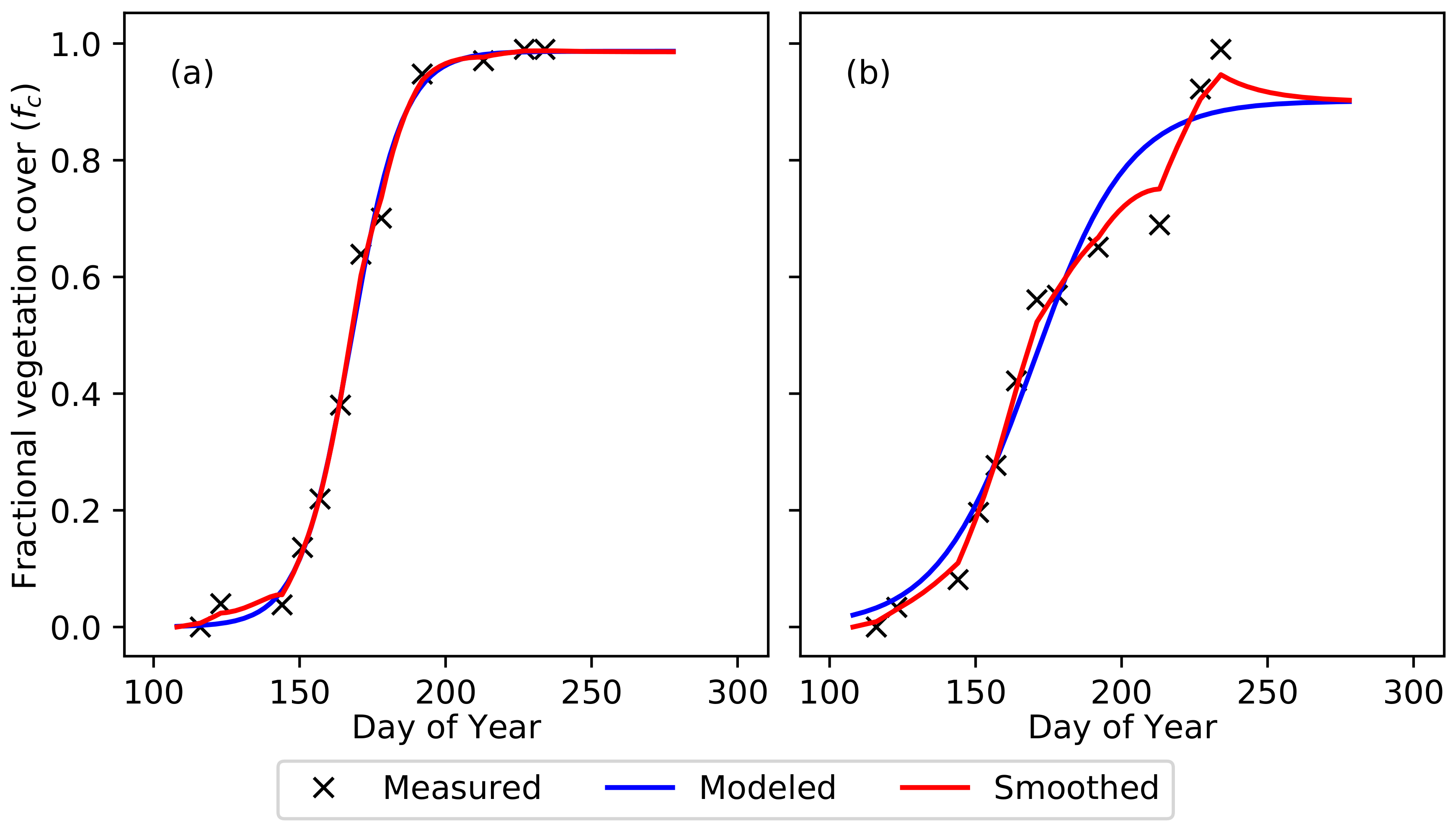
2.3. Fractional Cover Modeling

To facilitate calculations of cotton water use for each field plot (discussed below), daily f c estimates were obtained using a Kalman smoothing algorithm [30] to integrate drone-based f c measurements with f c from a daily logistic growth model:
f c t = r f c 1 - f c f c , max ,
where r describes the growth rate (d - 1 ) and f c , max is the maximum value that f c attains. This differential equation has an analytical solution:
f c = c e r ( t - t 0 ) 1 + c f c , max e r ( t - t 0 ) ,
where
c = f c , max f c , 0 f c , max - f c , 0
and f c , 0 is f c at the initial time ( t 0 ). The model was parameterized for each field plot by adjusting r, f c , 0 , and f c , max to minimize error between modeled f c and the drone-based f c measurements. The t 0 term was fixed as the DOY for planting each plot. Subsequently, Equation (3) with fitted parameters was incorporated into an unscented Kalman smoothing algorithm to develop daily f c time series that considered uncertainty in both the measured and modeled f c data. Kalman smoothing was especially important for characterizing f c in plots where the imposed treatments caused atypical growth patterns (Figure 2). To achieve reasonable time series as assessed visually, the f c state transition variance was set to 0.0002 while the measurement variance was set five times higher at 0.001. A Python script was developed to conduct this analysis, which incorporated a Nelder–Mead optimizer within the “scipy” package for parameter fitting and the “pykalman” package for unscented Kalman smoothing.

2.4. Crop Water Use Estimation

The daily f c time series from Kalman smoothing were rescaled to formulate basal crop coefficient (Kcb) time series, which were used to drive an ET-based daily soil water balance model as described in the Food and Agriculture Organization of the United Nations Paper No. 56 (FAO-56) [17]. Briefly, daily crop water use (ETc) was calculated with the following equation:
ET c = K c b K s + K e ET o s ,
where ETos is the standardized short crop reference evapotranspiration [31], Ke is the soil water evaporation coefficient, and Ks describes the effect of water stress on transpiration. Daily ETos was computed using data from an Arizona Meteorological Network station (AZMET) approximately 1.2 km from the field site. Required meteorological measurements included the daily minimum and maximum air temperature, dew point temperature, solar irradiance, and wind speed. Based on recommended computations for maximum Kcb given environmental data for Maricopa, the Kcb time series were rescaled from f c with a minimum value of 0.15 and maximum value of 1.225. The coefficients Ke and Ks were calculated as described in FAO-56. For Ks in particular, calculations were based on a daily soil water balance methodology, where soil water holding limits define the total plant available water. Under non-stressed conditions with root zone soil water at the drained upper limit, Ks is 1.0 and has no effect on ETc calculations (Equation (6)). As soil water is depleted, reductions in Ks are calculated, which lead to decreased ETc from plant transpiration. As mentioned above, the soil water holding limits were specified uniquely for each treatment plot based on soil sampling, soil texture analysis, pedotransfer function evaluations, and geostatistical calculations at the field site. Thus, the crop water use calculations were based on plot-level, site-specific information for both the soil water holding properties and the plant growth impacts on Kcb as characterized through drone-based f c . The soil water status on day i was calculated as follows:
D i = D i - 1 - P i - I i + ET c i + DS i ,
where D is the depth of root zone soil water depletion from the drained upper limit at the end of the day, P and I are the precipitation and irrigation received on the day, ETc is the daily crop water use from Equation (6), and DS is the water lost to deep seepage, which is calculated when water inputs exceed the root zone soil water storage capacity. This ET-based soil water balance model, as described in FAO-56 [17], was coded as a Python script for use in all cotton water use calculations in this study.
For each treatment plot in both field experiments in both growing seasons, ETc calculations were initiated on the day of planting and terminated after crop maturity in the first week of October. To summarize the seasonal crop water use, daily ETc calculations were aggregated over time. For comparison to measured ETc data in the irrigation management study (Equation (1)), daily ETc calculations were aggregated from the first to the last neutron moisture meter measurement dates in each growing season. For the cotton breeding trial, ETc data were aggregated over the entire calculation period from planting to crop maturity. Furthermore, seasonal CWUE (kg m - 3 ) was calculated from the ratio of measured cotton fiber yield and modeled seasonal cotton ET. To eliminate the effect of surface soil water evaporation, seasonal water use efficiency was also computed considering only the transpiration component of ET (TWUE, kg m - 3 ).

2.5. Statistical Analysis

Statistical software (SAS for Windows, ver. 9.3, SAS Institute, Cary, NC, USA) was used to fit a linear model for each of eleven cotton traits in response to the experimental treatments in the breeding trial. The eleven cotton traits were fiber yield (FY, kg ha - 1 ), seasonal evapotranspiration (ET, mm), crop water use efficiency (CWUE = FY:ET, kg m - 3 ), seasonal transpiration (T, mm), transpiration water use efficiency (TWUE = FY:T, kg m - 3 ), micronaire (MIC, unitless), upper half mean fiber length (UHM, mm), uniformity index (UI, mm mm - 1 ), fiber strength (STR, HVI g tex - 1 ), fiber elongation at failure (ELO, %), and short fiber content (SFC, %). Mixed model analysis of variance was conducted for each trait using the SAS MIXED procedure with the restricted maximum likelihood (REML) method. In the case that more than one trait estimate was available per plot, the plot mean was used as the dependent variable. The statistical model for each trait (Y) was
Y i j k l m n = μ + α i + β j + γ k + δ l ( k ) + ( α β ) i j + ( α γ ) i k + ( β γ ) j k + ( α δ ) i l ( k ) + ( β δ ) j l ( k ) + ( α β γ ) i j k + ( α β δ ) i j l ( k ) + ζ m + ( α ζ ) i m + ϵ n ( i j k l m ) ,
where experimental year ( α i ), cotton cultivar ( β j ), planting date ( γ k ), irrigation treatment nested within planting date ( δ l ( k ) ), and corresponding interaction terms were fitted as fixed effects, and the replicate ( ζ m ) and year by replicate interaction ( ( α ζ ) i m ) were fitted as random effects. To examine associations among traits, Pearson’s correlation coefficients (r) were determined using the SAS CORR procedure.

3. Results

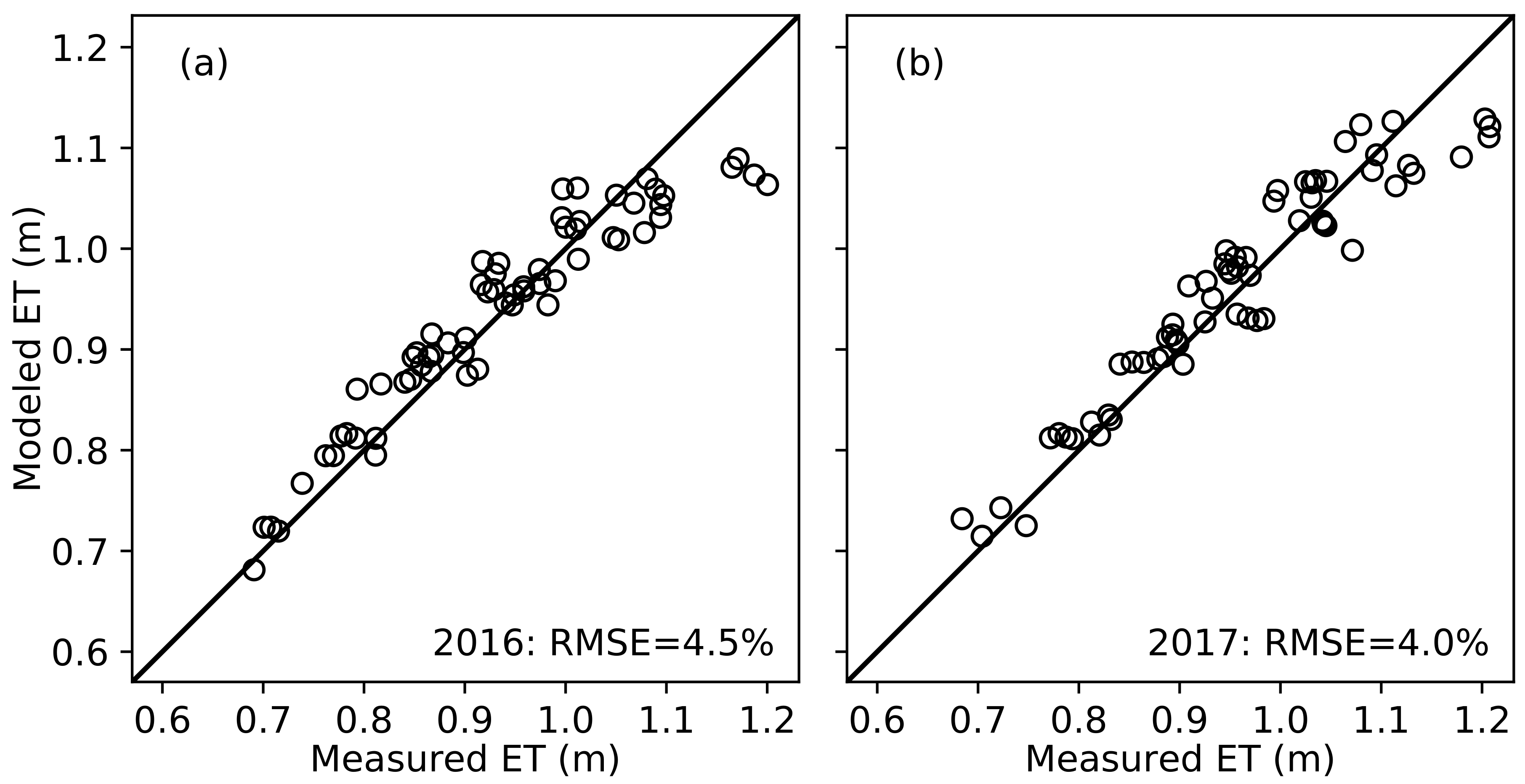
3.1. Crop Water Use Evaluation

Evaluation of seasonal cotton water use estimates from the drone-based ET modeling approach as compared to ET measurements from neutron moisture meters demonstrated reasonable performance with the modeling technique (Figure 3). The root mean squared errors (RMSE) between measured and modeled seasonal ET among 64 treatment plots in the irrigation management study were less than 5%. In both seasons, the model underestimated ET for the four treatment plots with the highest ET amounts. These treatment plots received 120% of the recommended irrigation rate over the whole season and were therefore overwatered. One possibility is that measured ET from the neutron moisture meters was overestimated, which is likely considering that deep seepage was estimated from soil moisture states typically one week apart (Equation (2)). In actuality, more water flux to deep seepage may have occurred for the overwatered plots, which would reduce estimates for measured ET (Equation (1)) if it could be accurately measured. For other treatment plots, which were not overwatered for the entire season, the agreement between measured and modeled ET was very good. In 2016 and 2017, measured deep seepage ranged from 45 to 97 mm and from 21 to 63 mm, respectively (not shown). Modeled deep seepage in both years ranged from 0 to 146 mm with a majority of plots modeled as having zero seepage. On average, measured deep seepage was less than 7% and 4% of ET in 2016 and 2017, respectively, which demonstrates the high importance of crop water use as a pathway for water loss from the agroecosystem. Overall, the results show that the drone-based f c and soil water balance modeling approach could effectively estimate seasonal cotton water use at this field site.

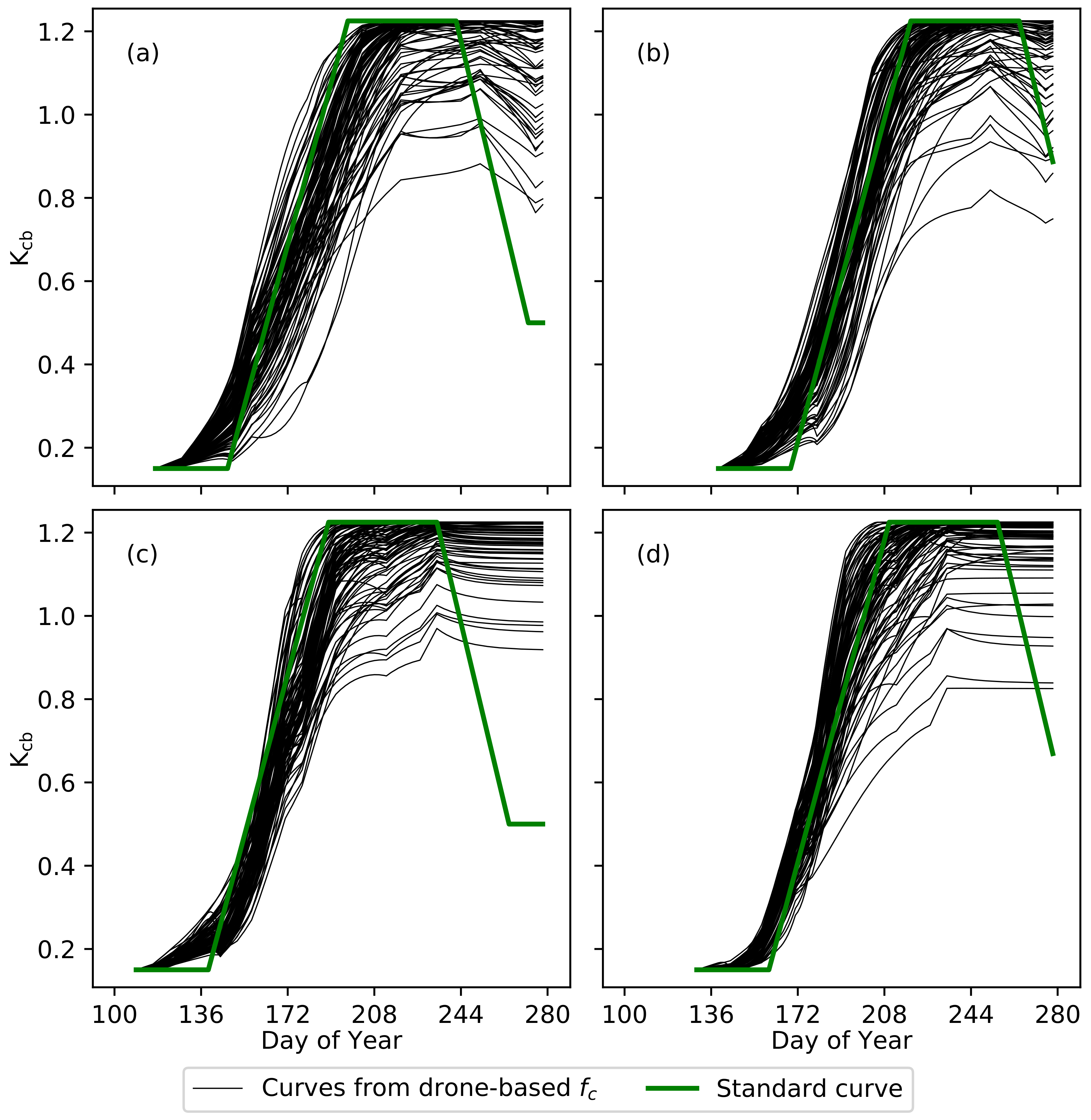
3.2. Basal Crop Coefficients

The basal crop coefficient (Kcb) time series for each plot in the breeding trial were variable according to the combined effect of planting date, irrigation rate, and cotton cultivar on f c , as measured using drone-based images (Figure 4). For example on DOY 184 in 2016, which is approximately the date of first flower, the Kcb among plots in the first planting varied from 0.40 to 1.09 (Figure 4a). This means that some plots were transpiring as low as 23% of full transpiration capacity on this day, while others were transpiring as high as 88% of full capacity. As compared to the standard trapezoidal Kcb time series, which were computed based on days after planting as recommended in FAO-56, many plots reached full transpiration capacity earlier than the standard, while others never reached full transpiration capacity. The drone-based f c data also suggested that late season Kcb remained higher than the standard Kcb recommendation, which may be true because cotton was traditionally a perennial plant and for agronomic purposes requires defoliation by desiccant application to terminate leaf growth and transpiration. Overall, to the extent that Kcb via drone-based f c correlates to plant transpiration rates, the data suggest highly variable water use patterns among the treatments imposed in the cotton breeding trial.

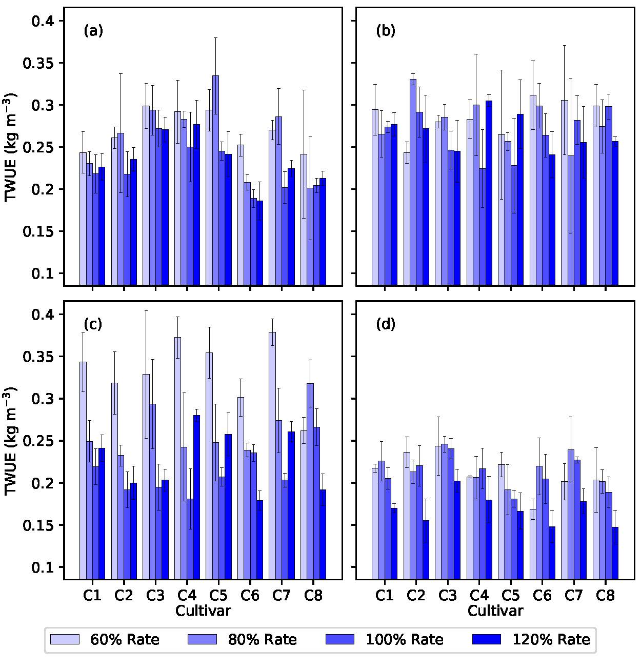
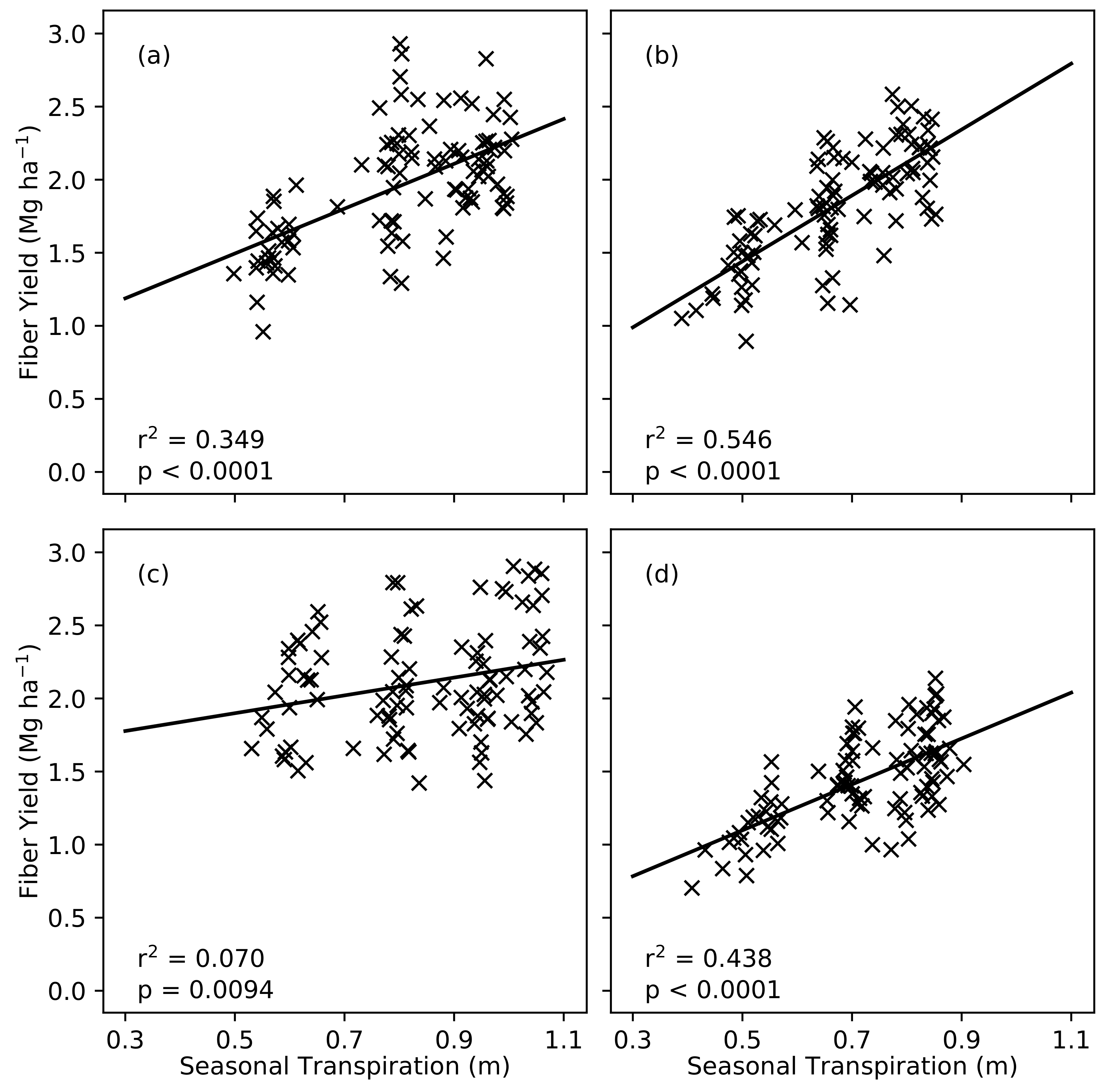
3.3. Statistical Results

Mean cotton fiber yield was 1831 kg ha - 1 and ranged from 703 to 2929 kg ha - 1 (Table 3), as measured in the cotton breeding trial for two growing seasons, two planting dates, and four irrigation rates. Computations of seasonal ET with the drone-based f c and soil water balance modeling approach ranged from 661 to 1223 mm, indicating that some plots used up to twice as much water as others. Estimates of the seasonal transpiration component of ET ranged from 389 to 1069 mm. On average, 0.19 kg of cotton fiber was produced per m 3 of water consumed (i.e., CWUE). Considering only the transpiration component of ET, mean TWUE was 0.25 kg m - 3 , a 26% increase as compared to calculations that included surface evaporation. This establishes an upper limit on the potential for CWUE improvements through management practices that reduce surface evaporation.
The fiber quality measurements suggested desirable fiber characteristics in some cases and less desirable characteristics in others. With micronaire values above 4.3, none of the plots produced fiber with micronaire in the range required for premium pricing (i.e., 3.7 to 4.2). Upper half mean length ranged from 26 to 32 mm, indicating medium to long fiber lengths. Uniformity indices ranged from 79 to 86 mm mm - 1 , indicating average to high fiber length uniformity. Fiber strength ranged from 27 to 40 HVI g tex - 1 , indicating average to very strong fibers. Elongation at failure ranged from 4.0% to 7.6%, indicating very low to high fiber elongation and an overall wide range for this study. With r equal to 0.31 and 0.33 (not shown), CWUE and TWUE, respectively, were correlated with fiber elongation at failure. Thus, the plots with higher water use efficiency tended to produce fibers that could stretch more before breaking. In addition, with r equal to 0.30 and 0.34, seasonal ET and T, respectively, were correlated with upper half mean fiber length. Thus, plots with higher water use generally produced longer fibers. Fiber yield did not correlate with any fiber quality metrics with r greater than 0.24. Thus, CWUE and TWUE were better estimators of fiber quality metrics than fiber yield in some cases.
Linear mixed modeling identified many differences ( p < 0 . 05 ) for the eleven cotton traits in response to the treatments imposed with the cotton breeding trial (Table 4). Mean FY, ET, CWUE, T and TWUE were different in the two growing seasons. However, among the fiber quality traits, only UI was different with growing season. The two planting date treatments led to differences in most of the cotton traits, with the exception of two fiber quality traits, STR and SFC. Likewise, irrigation rate led to differences in all traits except for the STR fiber quality trait. Differences among the eight cotton cultivars were found for all eleven cotton traits. Fiber yield and ET were different for all the interaction terms included in the model (Equation (8)), while the remaining cotton traits were occasionally different for these interactions (not shown). Most importantly, the mixed modeling results show that the methodology used to estimate cotton water use and CWUE led to differences for these traits among the eight cultivars. Thus, the approach may have value for breeding programs that aim to improve CWUE and identify drought tolerant cultivars.

3.4. Relevance to Breeding

Improving CWUE via plant breeding requires the identification of cultivars that yield highly but with reduced transpiration. An important aspect of the modeling methodology is that the crop coefficients (Equation (6)) permit partitioning of water use among plant transpiration and surface evaporation components. Thus, for purposes of breeding, the results can be discussed in terms of TWUE, the crop yield per volume of water transpired because breeding will primarily improve CWUE through the transpiration component of ET.
Plots of fiber yield versus seasonal transpiration demonstrated a positive correlation for all growing season and planting date combinations (Figure 5), generally equating higher yield with higher water use as commonly shown in crop water production functions [3]. Coefficients of determination ( r 2 ) between fiber yield and seasonal transpiration were higher with the second planting than with the first planting, indicating water management was a stronger driver of yield variability with later planting. Both fiber yield and seasonal transpiration were reduced with the second planting as compared to the first planting. The effect was due in part to a shorter growing season for the second planting because it was planted approximately one month later than the first planting while irrigation for both planting date treatments was terminated at the same time in early September. Extending the irrigation period later into September may have increased fiber yield and transpiration for the second planting.
Reduction in seasonal transpiration for the second planting may also be due to environmental differences. In central Arizona, the month of June (DOY 152 to 181) typically has high ambient temperatures and low humidity, which leads to increased evaporative demand (i.e., ETos). In addition, as seen in Figure 4, the Kcb (i.e., transpiration rate) during this period was much higher for the first planting than for the second planting due to higher f c . Thus, water use in the month of June was much greater for the first planting (Equation (6)). With the second planting, the hot and dry period in June was largely avoided, and maximum Kcb was not attained until July when the Arizona monsoon season brought higher humidity, reduced ambient air temperatures, and lower evaporative demand. Thus, improvements in CWUE may come from better timing of the maximum Kcb period with the Arizona monsoon season. Furthermore, because r 2 between fiber yield and transpiration was greater for the second planting, the Arizona monsoon season may provide a better environment for selecting heritable traits that improve yield and CWUE and increase genetic gain in breeding populations.
The calculated TWUE for each cotton variety in the breeding trial showed significant variation among planting dates and irrigation rates (Figure 6). The TWUE for the first 2017 planting at the 60% irrigation rate was unreasonably high (Figure 6c). This was likely due to errant irrigation applications to those plots, which was supported by soil moisture measurements (data not shown). After removing this treatment from consideration, DP1044B2RF (C3) and Arkot9704 (C2) demonstrated the most consistent TWUE across years, planting dates, and irrigation treatments. Furthermore, C3 was ranked as the second highest yielding line and also had consistent fiber quality traits across years and treatments. This means producers should expect consistent yields with C3 and C2 over a range of soil water status conditions. However, selecting on yield stability alone can be unreliable due to the effects of environmental variation across growing seasons. Calculated TWUE may provide an alternative phenotype for selection because aggregated environmental conditions are included in the estimate, thus reducing selection error caused by environment or management variation. For example, DP1044B2RF (C3) and FM958 (C5) consistently achieved higher TWUE at the 80% irrigation level as compared to the higher irrigation levels, which may highlight commercial breeders’ efforts to select for drought tolerance in the development of these varieties.

4. Discussion

A main advantage of the ET-based soil water balance model (Equations (6) and (7)) is its partitioning of crop water use into surface evaporation and plant transpiration components via crop coefficients (Kcb, Ks, and Ke). As dictated by the model equations [17], Ks and Ke are mainly influenced by soil water holding characteristics, and Ke is additionally influenced by the irrigation system and ground cover. Thus, reductions in crop water use via changes to these coefficients can be achieved only through adjustments in management practices. Some options include switching to subsurface drip irrigation to limit surface evaporation, adopting conservation tillage to increase ground cover, or using variable-rate irrigation to adjust irrigation rates based on the site-specific soil water holding characteristics. The remaining coefficient, Kcb, is the primary driver of plant transpiration in the model. As such, reductions in crop water use via changes to Kcb can be achieved mainly through plant breeding. The goal for breeding should be to select varieties that yield highly while exhibiting Kcb time series (Figure 4) that reduce water use through transpiration. By incorporating models of cropping system processes into crop breeding and management efforts, the improvements offered by management versus breeding can be better quantified.
The present study achieved high-throughput phenotyping of crop water use efficiency using relatively simple imaging and modeling technologies. Obviously, plant transpiration is dictated by processes with higher complexity than can be described through f c time series alone. For example, the processes of root water uptake, water transport through the plant, leaf stomatal conductance, and other plant water regulatory mechanisms are not considered in this study. Incorporation of more complex models that consider plant water status in greater detail may improve transpiration estimates, although models with higher complexity often also increase the model parameterization requirements. To be effective, the model parameters would need to be accurately estimated, or perhaps phenotyped, for each variety, which could be the subject of future studies. In this study, a simpler model was chosen due to the relative ease of driving the model with basic f c measurements from drone-based multispectral imaging. A main contribution is the use of time-series f c estimates with a simple soil water balance model to provide seasonal transpiration estimates for breeding trials at the plot-level. As such, the relatively simple methodology provides a practical way to incorporate information on crop water use into decisions on breeding selection and may be especially useful when the goal is to simply determine which varieties to keep in the breeding program.
As this study represents one of several initial efforts with drone-based imaging at the Maricopa research station, much has been learned over the duration of the study. Regarding the choice of sensors, the commercial multispectral cameras (i.e., Micasense RedEdge and Parrot Sequoia) were popular products marketed for the agricultural sector at the time of the study, and they were therefore given primary focus for flight hours. As such, the data from these sensors more fully covered the growing season as required for time-series f c estimates herein. An astute reader will note that f c time series could perhaps be more easily attained from digital color (RGB) cameras, which is a simpler and more pervasive imaging technology with greater commercial options for choices of camera and drone platform. Additionally, the image spatial resolution is often higher for RGB cameras, and image calibration methods are simpler as compared to multispectral image calibration. Data from RGB cameras were also collected over the field site but with less frequency and consistency, which made these data less useful for the study. Because the Parrot Sequoia camera collected both RGB and multispectral data, efforts with this camera in 2017 (Table 2) aimed to collect both types of data in a single drone flight. However, the success of this approach was reduced by data reliability issues with the camera and multiple crashes of the fixed-wing drone for which the camera was designed. Hence, the MicaSense RedEdge camera on a custom hexacopter drone was the favored configuration herein. For future efforts to map f c time series, an even better configuration may be an RGB camera on a copter-style drone, for which there are now many commercial options. However, future studies should also further contrast the advantages and disadvantages of multispectral versus RGB imaging from drone platforms.
Missing from this study is the use of thermal cameras to quantify differences in plant water status among varieties, which again was related to giving primary focus for flight hours to the multispectral cameras. Incorporating canopy temperature information from thermal cameras into the methodology has great potential to improve transpiration estimates among varieties. For example, Kullberg et al. [32] recently described the use of stationary infrared thermometry to adjust Ks in the ET-based soil water balance model (Equation (6)), applied to maize. Although their data was collected from ground-based systems rather than drones, their approach demonstrates the integration of Kcb from RGB data and Ks from thermal data into the ET-based soil water balance model for quantifying maize water use. Future efforts should evaluate this data fusion technique for improved high-throughput phenotyping of crop water use among crop varieties, likely using RGB and thermal data from drone-based images or sensors mounted on ground-based phenotyping vehicles [25].

5. Conclusions

High-throughput phenotyping of water use in 192 cotton breeding plots was achieved using approximately weekly vegetation cover estimates from drone-based multispectral cameras to drive basal crop coefficients in a daily soil water balance model. Differences in water use estimates among eight cotton cultivars were found via linear mixed modeling, indicating that the approach can assist breeders in the identification of cultivars with favorable water use characteristics. Combining the water use estimates with crop yield can quantify crop water use efficiency, allowing breeders to select varieties that maximize crop production per volume of water used. Options for improving the methodology include considering models with greater complexity in crop water use processes, assessing alternative options for drone-based image data collection, and incorporating other crop phenotypes such as canopy temperature. Taken together, the study demonstrates a methodology for high-throughput phenotyping of crop water use, providing breeders a tool for water use quantification and additional traits for consideration in selective breeding.

Author Contributions

Conceptualization, K.R.T. and A.L.T.; Methodology, All authors; Software, K.R.T., S.J.H., and A.N.F.; Validation, All authors; Formal Analysis, K.R.T. and A.L.T.; Investigation, All authors; Resources, R.W.W.; Data Curation, K.R.T.; Writing—Original Draft Preparation, K.R.T. and A.L.T.; Writing—Review and Editing, All authors; Visualization, K.R.T. and A.L.T.; Supervision, K.R.T., A.N.F., and R.W.W.; Project Administration, K.R.T. and R.W.W.; Funding Acquisition, K.R.T. and R.W.W.

Funding

This research was partially funded by Cotton Incorporated.

Acknowledgments

The authors acknowledge Mark Yori from Phoenix Drone Services for collection of multispectral drone imagery for this research. In addition, the authors acknowledge the USDA-ARS-ALARC technicians and summer employees for conducting field experiments and collecting field data to support this research, including Suzette Maneely, Bill Luckett, Matt Hagler, Melissa Stefanek, Cassie Farwell, Josh Cederstrom, Matthew McGuire, Dusti Baker, and Joseph Griffin.

Conflicts of Interest

The authors declare no conflict of interest. The founding sponsors had no role in the design of the study; in the collection, analyses, or interpretation of data; in the writing of the manuscript, and in the decision to publish the results.

References

  1. Dai, A. Drought under global warming: A review. Wiley Interdiscip. Rev. Clim. Chang. 2011, 2, 45–65. [Google Scholar] [CrossRef]
  2. Wehner, M.; Easterling, D.R.; Lawrimore, J.H.; Heim, R.R.; Vose, R.S.; Santer, B.D. Projections of future drought in the continental United States and Mexico. J. Hydrometeorol. 2011, 12, 1359–1377. [Google Scholar] [CrossRef]
  3. Ali, M.H.; Talukder, M.S.U. Increasing water productivity in crop production—A synthesis. Agric. Water Manag. 2008, 95, 1201–1213. [Google Scholar] [CrossRef]
  4. Passioura, J.B. Phenotyping for drought tolerance in grain crops: When is it useful to breeders? Funct. Plant Biol. 2012, 39, 851–859. [Google Scholar] [CrossRef]
  5. Evans, R.G.; King, B.A. Site-specific sprinkler irrigation in a water-limited future. Trans. ASABE 2012, 55, 493–504. [Google Scholar] [CrossRef]
  6. Sadler, E.J.; Evans, R.G.; Stone, K.C.; Camp, C.R. Opportunities for conservation with precision irrigation. J. Soil Water Conserv. 2005, 60, 371–379. [Google Scholar]
  7. Araus, J.L.; Cairns, J.E. Field high-throughput phenotyping: The new crop breeding frontier. Trends Plant Sci. 2014, 19, 52–61. [Google Scholar] [CrossRef] [PubMed]
  8. Chapman, S.C.; Chakraborty, S.; Dreccer, M.F.; Howden, S.M. Plant adaptation to climate change–opportunities and priorities in breeding. Crop Pasture Sci. 2012, 63, 251–268. [Google Scholar] [CrossRef]
  9. Gago, J.; Douthe, C.; Coopman, R.E.; Gallego, P.P.; Ribas Carbo, M.; Flexas, J.; Escalona, J.; Medrano, H. UAVs challenge to assess water stress for sustainable agriculture. Agric. Water Manag. 2015, 153, 9–19. [Google Scholar] [CrossRef]
  10. Gowda, P.H.; Chavez, J.L.; Colaizzi, P.D.; Evett, S.R.; Howell, T.A.; Tolk, J.A. ET mapping for agricultural water management: Present status and challenges. Irrig. Sci. 2008, 26, 223–237. [Google Scholar] [CrossRef]
  11. Khanal, S.; Fulton, J.; Shearer, S. An overview of current and potential applications of thermal remote sensing in precision agriculture. Comput. Electron. Agric. 2017, 139, 22–32. [Google Scholar] [CrossRef]
  12. Maes, W.H.; Steppe, K. Estimating evapotranspiration and drought stress with ground-based thermal remote sensing in agriculture: A review. J. Exp. Biol. 2012, 63, 4671–4712. [Google Scholar] [CrossRef] [PubMed]
  13. Wesseling, J.G.; Feddes, R.A. Assessing crop water productivity from field to regional scale. Agric. Water Manag. 2006, 86, 30–39. [Google Scholar] [CrossRef]
  14. Yebra, M.; Van Dijk, A.; Leuning, R.; Huete, A.; Guerschman, J. Evaluation of optical remote sensing to estimate actual evapotranspiration and canopy conductance. Remote Sens. Environ. 2013, 129, 250–261. [Google Scholar] [CrossRef]
  15. Colaizzi, P.D.; O’Shaughnessy, S.A.; Evett, S.R.; Mounce, R.B. Crop evapotranspiration calculation using infrared thermometers aboard center pivots. Agric. Water Manag. 2017, 187, 173–189. [Google Scholar] [CrossRef] [Green Version]
  16. Hunsaker, D.J.; French, A.N.; Waller, P.M.; Bautista, E.; Thorp, K.R.; Bronson, K.F.; Andrade Sanchez, P. Comparison of traditional and ET-based irrigation scheduling of surface-irrigated cotton in the arid southwestern USA. Agric. Water Manag. 2015, 159, 209–224. [Google Scholar] [CrossRef]
  17. Allen, R.G.; Pereira, L.S.; Raes, D.; Smith, M. FAO Irrigation and Drainage Paper No. 56. Crop Evapotranspiration: Guidelines for Computing Crop Water Requirements; Food and Agriculture Organization of the United Nations: Rome, Italy, 1998. [Google Scholar]
  18. Zaman-Allah, M.; Vergara, O.; Araus, J.L.; Tarekegne, A.; Magorokosho, C.; Zarco-Tejada, P.J.; Hornero, A.; Albà, A.H.; Das, B.; Craufurd, P.; et al. Unmanned aerial platform-based multi-spectral imaging for field phenotyping of maize. Plant Methods 2015, 11, 35. [Google Scholar] [CrossRef] [PubMed]
  19. Sankaran, S.; Khot, L.R.; Carter, A.H. Field-based crop phenotyping: Multispectral aerial imaging for evaluation of winter wheat emergence and spring stand. Comput. Electron. Agric. 2015, 118, 372–379. [Google Scholar] [CrossRef]
  20. Condorelli, G.E.; Maccaferri, M.; Newcomb, M.; Andrade-Sanchez, P.; White, J.W.; French, A.N.; Sciara, G.; Ward, R.; Tuberosa, R. Comparative aerial and ground based high throughput phenotyping for the genetic dissection of NDVI as a proxy for drought adaptive traits in durum wheat. Front. Plant Sci. 2018, 9, 893. [Google Scholar] [CrossRef] [PubMed]
  21. El-Hendawy, S.E.; Hassan, W.M.; Al-Suhaibani, N.A.; Schmidhalter, U. Spectral assessment of drought tolerance indices and grain yield in advanced spring wheat lines grown under full and limited water irrigation. Agric. Water Manag. 2017, 182, 1–12. [Google Scholar] [CrossRef]
  22. Rischbeck, P.; Elsayed, S.; Mistele, B.; Barmeier, G.; Heil, K.; Schmidhalter, U. Data fusion of spectral, thermal and canopy height parameters for improved yield prediction of drought stressed spring barley. Eur. J. Agron. 2016, 78, 44–59. [Google Scholar] [CrossRef]
  23. Thorp, K.R.; Gore, M.A.; Andrade Sanchez, P.; Carmo Silva, A.E.; Welch, S.M.; White, J.W.; French, A.N. Proximal hyperspectral sensing and data analysis approaches for field-based plant phenomics. Comput. Electron. Agric. 2015, 118, 225–236. [Google Scholar] [CrossRef] [Green Version]
  24. Winterhalter, L.; Mistele, B.; Jampatong, S.; Schmidhalter, U. High throughput phenotyping of canopy water mass and canopy temperature in well-watered and drought stressed tropical maize hybrids in the vegetative stage. Eur. J. Agron. 2011, 35, 22–32. [Google Scholar] [CrossRef]
  25. White, J.W.; Andrade Sanchez, P.; Gore, M.A.; Bronson, K.F.; Coffelt, T.A.; Conley, M.M.; Feldmann, K.A.; French, A.N.; Heun, J.T.; Hunsaker, D.J.; et al. Field-based phenomics for plant genetics research. Field Crops Res. 2012, 133, 101–112. [Google Scholar] [CrossRef]
  26. Gee, G.W.; Bauder, J.W. Partical-size analysis. In Methods of Soil Analysis, Part 1. Physical and Mineralogical Methods; ASA-SSSA: Madison, WI, USA, 1986; Chapter 15; pp. 383–411. [Google Scholar]
  27. Zhang, Y.; Schaap, M.G. Weighted recalibration of the Rosetta pedotransfer model with improved estimates of hydraulic parameter distributions and summary statistics (Rosetta3). J. Hydrol. 2017, 547, 39–53. [Google Scholar] [CrossRef]
  28. Thorp, K.R.; Hunsaker, D.J.; Bronson, K.F.; Andrade-Sanchez, P.; Barnes, E.M. Cotton irrigation scheduling using a crop growth model and FAO-56 methods: Field and simulation studies. Trans. ASABE 2017, 60, 2023–2039. [Google Scholar] [CrossRef]
  29. Hunsaker, D.J.; Barnes, E.M.; Clarke, T.R.; Fitzgerald, G.J.; Pinter, P.J. Cotton irrigation scheduling using remotely sensed and FAO-56 basal crop coefficients. Trans. ASAE 2005, 48, 1395–1407. [Google Scholar] [CrossRef]
  30. Kalman, R.E. A new approach to linear filtering and prediction problems. J. Basic Eng. 1960, 82, 35–45. [Google Scholar] [CrossRef]
  31. Walter, I.A.; Allen, R.G.; Elliott, R.; Itenfisu, D.; Brown, P.; Jensen, M.E.; Mecham, B.; Howell, T.A.; Snyder, R.; Eching, S.; et al. The ASCE Standardized Reference Evapotranspiration Equation; ASCE-EWRI: Reston, VA, USA, 2005. [Google Scholar]
  32. Kullberg, E.G.; DeJonge, K.C.; Chávez, J.L. Evaluation of thermal remote sensing indices to estimate crop evapotranspiration coefficients. Agric. Water Manag. 2017, 179, 64–73. [Google Scholar] [CrossRef]
Figure 1. Experimental layouts for (1) a large-plot cotton irrigation management study with soil water content measurements at 64 access tube locations (Experiment #1) and (2) a small-plot cotton study comparing two planting dates (P1 and P2) with eight cotton cultivars and four irrigation rates (Experiment #2) in the (a) 2016 and (b) 2017 growing seasons at Maricopa, AZ, USA. Seasonal irrigation rates (mm) for each plot area are shown with false color composite images of the field on (a) 21 July 2016 and (b) 15 August 2017.
Remotesensing 10 01682 g001
Figure 2. Daily fractional vegetation cover ( f c ) estimation using Kalman smoothing to integrate drone-based f c measurements with a daily logistic growth model for plots that received (a) the recommended irrigation schedule and (b) a schedule that underwatered early and overwatered late in the 2017 growing season at Maricopa, AZ, USA.
Remotesensing 10 01682 g002
Figure 3. Modeled versus measured cotton evapotranspiration (ET) for the 64 irrigation management plots from day of year (a) 138 to 277 in 2016 and (b) 129 to 274 in 2017 at Maricopa, AZ, USA.
Remotesensing 10 01682 g003
Figure 4. Basal crop coefficients (Kcb) as estimated from drone-based fractional vegetation cover ( f c ) in the (a) first and (b) second planting in 2016 and the (c) first and (d) second planting in 2017 for breeding trials conducted in Maricopa, AZ, USA. The standard trapezoidal Kcb curve as recommended in FAO-56 is presented for comparison.
Remotesensing 10 01682 g004
Figure 5. Cotton fiber yield versus seasonal transpiration for 96 treatment plots (4 irrigation rates × 8 cotton cultivars × 3 replications = 96 plots) with (a) the first planting date in 2016; (b) the second planting date in 2016; (c) the first planting date in 2017; and (d) the second planting date in 2017. Data were collected as part of a cotton breeding trial conducted at Maricopa, AZ, USA.
Remotesensing 10 01682 g005
Figure 6. Transpiration water use efficiency (TWUE) for eight cotton cultivars (C1, Ark071209; C2, Arkot9704; C3, DP1044B2RF; C4, DP12R244R2; C5, DP1549B2XF; C6, FM958; C7, PD07040; C8, Siokra L23) at four irrigation rates (60%, 80%, 100%, and 120% of recommended amounts) for (a) the first planting date in 2016; (b) the second planting date in 2016; (c) the first planting date in 2017; and (d) the second planting date in 2017. Data were collected as part of a cotton breeding trial conducted at Maricopa, AZ, USA.
Remotesensing 10 01682 g006
Table 1. Summary of eight cotton cultivars planted in the cotton breeding trial during the 2016 and 2017 growing seasons at Maricopa, AZ, USA.
AbbreviationFull NameTypeSource
Ark071209Ark071209Breeding lineUniversity of Arkansas, Keiser, AR, USA
Arkot9704Arkot 9704Released germplasmUniversity of Arkansas, Keiser, AR, USA
DP1044B2RFDeltapine 1044 B2RFCommercial cultivarMonsanto Company, St. Louis, MO, USA
DP12R244R2Deltapine 1441 RFCommercial cultivarMonsanto Company, St. Louis, MO, USA
DP1549B2XFDeltapine 1549 B2XFCommercial cultivarMonsanto Company, St. Louis, MO, USA
FM958FiberMax 958Commercial cultivarBayer Crop Science, Raleigh, NC, USA
PD07040Pee Dee 07040Breeding lineUSDA-ARS, Florence, SC, USA
Siokra L23Siokra L23Improved varietyCSIRO, Canberra, ACT, Australia
Table 2. Multispectral image reconnaissance from unmanned aerial systems during the 2016 and 2017 cotton growing seasons at Maricopa, AZ, USA 1 .
DateDOYDAP1DAP2Camera
28 May 20161493210RedEdge
5 June 20161574018RedEdge
28 June 20161806341RedEdge
5 July 20161877048RedEdge
12 July 20161947755RedEdge
21 July 20162038664RedEdge
6 August 201621910280RedEdge
31 August 2016244127105RedEdge
8 September 2016252135113RedEdge
1 October 2016275158136RedEdge
3 May 201712314−7RedEdge
24 May 20171443514Sequoia
31 May 20171514221Sequoia
6 June 20171574827Sequoia
13 June 20171645534Sequoia
20 June 20171716241Sequoia
27 June 20171786948Sequoia
11 July 20171928362Sequoia
1 August 201721310483RedEdge
15 August 201722711897RedEdge
22 August 2017234125104RedEdge
1 day of year, DOY; days after the first planting, DAP1; days after the second planting, DAP2.
Table 3. Simple statistics for eleven cotton traits as measured for the 2016 and 2017 cotton breeding trials at Maricopa, AZ, USA, including cotton fiber yield (FY), seasonal evapotranspiration (ET), crop water use efficiency (CWUE = FY:ET), seasonal transpiration (T), transpiration water use efficiency (TWUE = FY:T), micronaire (MIC), upper half mean fiber length (UHM), uniformity index (UI), fiber strength (STR), fiber elongation at failure (ELO), and short fiber content (SFC).
TraitUnitnMeanStd DevMinimumMaximum
FYkg ha - 1 3831831.00445.16703.152929.00
ETmm384954.73145.07661.401223.00
CWUEkg m - 3 3830.190.040.100.31
Tmm384757.50158.85389.201069.00
TWUEkg m - 3 3830.250.050.130.40
MICunitless3845.170.304.306.00
UHMmm38428.961.0226.1631.50
UImm mm - 1 38482.791.0679.3085.80
STRHVI g tex - 1 38431.851.8627.2039.70
ELO%3845.870.824.007.60
SFC%3848.230.606.7010.70
Table 4. Linear mixed modeling results for the cotton breeding trial at Maricopa, AZ, USA, including F statistics and probability values (p) for cotton fiber yield (FY), seasonal evapotranspiration (ET), crop water use efficiency (CWUE = FY:ET), seasonal transpiration (T), transpiration water use efficiency (TWUE = FY:T), micronaire (MIC), upper half mean fiber length (UHM), uniformity index (UI), fiber strength (STR), fiber elongation at failure (ELO), and short fiber content (SFC).
TraitYearPlanting DateIrrigation RateCultivar
FpFpFpFp
FY21.870.0001273.970.000142.980.00015.310.0001
ET96.230.00015589.250.00013073.790.00012.250.0305
CWUE35.220.000138.790.000113.660.00015.220.0001
T127.660.00011272.990.0001941.460.00012.910.0061
TWUE39.420.000123.060.000141.590.00015.770.0001
MIC2.710.347411.350.00094.060.000715.700.0001
UHM10.830.052518.560.000128.660.00016.750.0001
UI54.690.00016.840.011211.310.00012.810.0079
STR0.010.93280.170.67765.190.000114.240.0001
ELO0.530.54798.750.00341.860.088417.840.0001
SFC0.240.63633.630.058012.090.00013.820.0006

