Classification of Hydrometeors Using Measurements of the Ka-Band Cloud Radar Installed at the Milešovka Mountain (Central Europe)

Abstract

In radar meteorology, greater interest is dedicated to weather radars and precipitation analyses. However, cloud radars provide us with detailed information on cloud particles from which the precipitation consists of. Motivated by research on the cloud particles, a vertical Ka-band cloud radar (35 GHz) was installed at the Milešovka observatory in Central Europe and was operationally measuring since June 2018. This study presents algorithms that we use to retrieve vertical air velocity (Vair) and hydrometeors. The algorithm calculating Vair is based on small-particle tracers, which considers the terminal velocity of small particles negligible and, thereby, Vair corresponds to the velocity of the small particles. The algorithm classifying hydrometeors consists of calculating the terminal velocity of hydrometeors and the vertical temperature profile. It identifies six hydrometeor types (cloud droplets, ice, and four precipitating particles: rain, graupel, snow, and hail) based on the calculated terminal velocity of hydrometeors, temperature, Vair, and Linear Depolarization Ratio. The results of both the Vair and the distribution of hydrometeors were found to be realistic for a thunderstorm associated with significant lightning activity on 1 June 2018.

1. Introduction

Measurements from a millimeter-wave Doppler radars are suitable for research on cloud microphysics at a high spatial and temporal resolution [1,2,3]. Therefore, a vertically pointing polarimetric Ka-band cloud radar (35 GHz) was installed at the Milešovka observatory (Czech Republic, Central Europe) as part of the running project Cosmic Rays and Radiation Events in the Atmosphere (CRREAT). CRREAT is focused on the relationships between cloud hydrometeors/precipitation particles and the electric field in the atmosphere. The Milešovka observatory is situated at a mountain top at an elevation of 837 m, which exceeds the surrounding landscape of more than 300 m and, thus, provides a 360° unobstructed view from the observatory. The observatory is equipped with a wide set of instruments (meteorological and non-meteorological) and its unique location and limited accessibility to the observatory counted among the reasons for selecting this type of cloud radar.

To the best of our knowledge, there are 17 Ka-band cloud radars operating in Europe (seven in Germany) including two mobile Ka-band cloud radars. The newly installed Ka-band cloud radar at the Milešovka observatory is the first of its kind operating in the Czech Republic. The installation of the radar at the observatory took place at the end of March 2018 and the radar started operating in June 2018.

The aim of this article is to describe two new functionalities that we added to the radar data processing to study the cloud structures, which is our research purpose. Specifically, we dealt with (i) the estimation of vertical air velocity and terminal velocity of hydrometeors and (ii) the classification of hydrometeors for which the vertical velocity and terminal velocity are the input parameters. Note that hydrometeors are any kind of liquid or solid water particles in the atmosphere that can result in precipitation, which may or may not reach the ground in the form of graupel, rain, snow, or hail.

Several pioneer studies that tried to retrieve the vertical air motion were often based on fixing an empirical relationship between the radar reflectivity and terminal velocity of hydrometeors depending on the diameter of hydrometeors [4,5]. However, a straightforward relationship among the variables is difficult to establish and is not known in the case of thunderclouds [6]. Kollias [7] applied a method for retrieving the vertical motion for W-band cloud radar that is valid for intense precipitation. The method was introduced by Lhermitte [8] and consists of retrieving the vertical air velocity from the signature of the observed Doppler spectra modulated by Mie scattering. However, Zheng et al. [6] pointed out that, by using measurements of millimeter (Ka/W) cloud radars, this method is not valid for the case of small particles including cloud droplets or light precipitation. In such a case, one can use the “small-particle-traced” method to retrieve the vertical air velocity [6]. The method assumes that small particles (i.e., tracers) have a negligible terminal velocity. Therefore, their velocity corresponds to that of the air [9,10,11]. This method was applied by Zheng et al. [6] during the TIPEX-III experiment over the Tibetan Plateau. Their retrieved air velocity was found to be reliable and in good agreement with other radar measurements and, as compared to retrievals based on disdrometer measurements, it provided more detailed information about the vertical air motion. Thus, we used this method in our study as well.

The classification of hydrometeors using cloud radar data has been discussed in many studies [12,13,14,15]. In general, hydrometeor classification algorithms using polarimetric measurements of any kind of Doppler radar can be based on the combination of radar reflectivity with a Linear Depolarization Ratio (LDR) and/or with differential reflectivity [16,17,18] or reflectivity difference [19]. In the past, the main target was the detection of hail from precipitation. In several studies [20,21], the hydrometeors were classified by using the decision tree method while, in others, by using fuzzy logic and neural networks [22]. Nowadays, most of the algorithms classifying hydrometeors using cloud radar data belong to the retrieving methods of Doppler spectra [12,13,23,24]. For instance, the retrieving methods for cloud properties were provided in Reference [25]. For upper tropospheric clouds, they have been compared in Reference [26] and, for stratospheric clouds, they were compared in Reference [27]. Other studies discussed the retrieving methods for cloud radar placed on satellites [28]. The algorithm that is used by the provider of our cloud radar was presented in Reference [29]. However, many classifying algorithms were either designed for weather radars (e.g., C-band) or limited to a specific kind of particle such as ice or precipitation.

In our study, we aim at classifying hydrometeors based mainly on the differences in terminal velocities of precipitating hydrometeors. The terminal velocity of hydrometeors suggests the occurrence of precipitation (the higher the terminal velocity of a hydrometeor, the higher the probability that the hydrometeor reaches the ground, i.e., precipitates). We illustrate the computational methods with an event that occurred on 1 June 2018. On 1 June 2018, a thunderstorm occurred near the Milešovka observatory producing many lightning strikes and precipitation at the observatory and its vicinity.

The article is organized as follows. After this introductory Section 1, Section 2 describes the Milešovka observatory and provides details about the Ka-band cloud radar installed at the observatory. Section 2 also depicts the thunderstorm on 1 June 2018 associated with strong lightning activity and it shows the radar data processing and the algorithms that we use to calculate the vertical air velocity and to classify the hydrometeors. Section 3 displays the resulting retrieved vertical air velocity and the distribution of hydrometeors during the thunderstorm on 1 June 2018 while Section 4 discusses the obtained results and compares it with those retrieved by the provided radar software. Conclusions are drawn in Section 5.

2. Materials and Methods

2.1. Milešovka Observatory

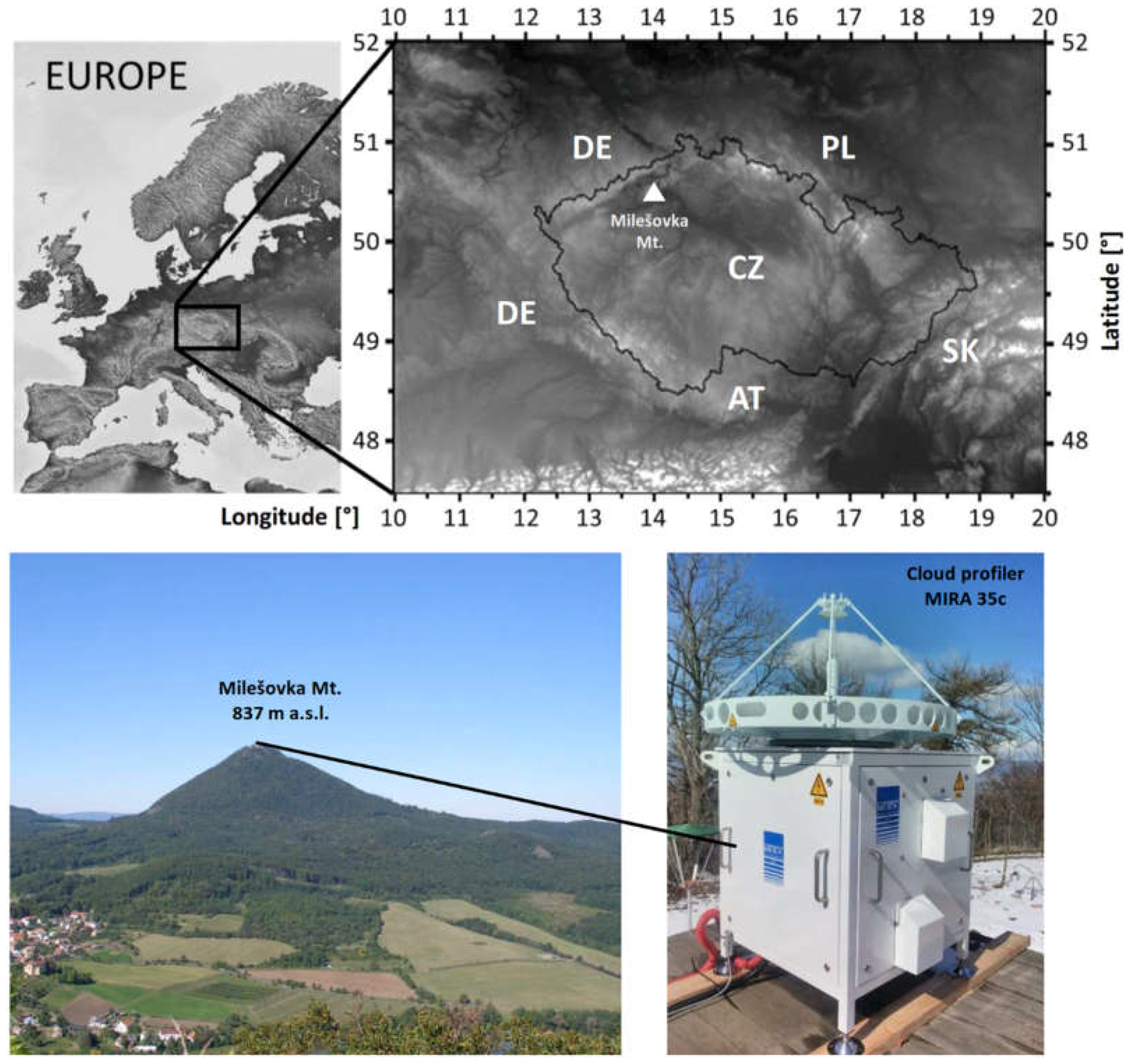
The Milešovka observatory is situated on the highest top of Central Bohemian Uplands in the Czech Republic in Central Europe (Figure 1) called the Milešovka Mountain (837 m a.s.l.; 50°33′18″N. and 13°55′54″E.). It is a meteorological and climatological observatory with continuous measurements since 1905. The location of the Milešovka observatory is suitable for atmospheric research due to a large 360° view and an absence of high obstacles in the surroundings, which makes it a unique meteorological observatory in the Czech Republic.

The Milešovka observatory is operated by the Institute of Atmospheric Physics, Czech Academy of Sciences and controlled by an observer with a 24/7 service. The equipment includes instruments of a standard meteorological and climatological station providing e.g., measurements of temperature, precipitation, and wind. Moreover, it also includes two sonic anemometers, Vaisala ceilometer CL51, Thies Laser Precipitation Monitor etc. Besides various meteorological instruments, the Milešovka observatory is also equipped with instruments measuring the atmospheric electric field (Boltek Electric Field Monitor EFM-100), the magnetic field (SLAVIA sensors, Shielded Loop Antenna with a Versatile Integrated Amplifier), and charged and neutral components of secondary cosmic rays (SEVAN) in order to investigate lightning in thunderstorms.

On 26 March 2018, a Ka-band vertically pointing cloud radar (profiler MIRA35c) was installed at the station (Figure 1) for detecting cloud particles in order to derive the distribution of hydrometeors in clouds. In clouds and thunderclouds, the hydrometeors might be responsible for precipitation and heavy rainfall, respectively.

2.2. Ka-Band Cloud Radar at the Milešovka Observatory

The Ka-band cloud radar (profiler MIRA35c) installed at the Milešovka observatory (Figure 1) was provided by METEK Gmbh (http://metek.de/). It is a Ka-band Doppler polarimetric radar with a center frequency of 35.12 +/−0.1 GHz. The cloud radar is vertically oriented and its technical specifications are listed in

Table 1. Technical specifications of the cloud radar MIRA35c installed at the Milešovka observatory.

Radar Parameter	MIRA35c
Radar system	Doppler polarimetric
Radar band	Ka
Transmitter frequency [GHz]	35.12 +/−0.1
Radar core	Magnetron
Peak power [W]	2500
Antenna type	Casse grain
Antenna diameter [m]	1
Antenna gain [dB]	48.5
Antenna beam width [°]	0.6
Pulse repetition frequency [Hz]	2500–10,000
Pulse width [ns]	min. 100, max. 400
Detection unambiguous velocity range [m·s−1]	±10.65
Original data measurements	Doppler spectra
Spectral moments	Reflectivity (Z)
	Doppler vertical velocity (DVV)
	spectrum width (σ)
Derived variables	Linear Depolarization Ratio (LDR)
	Signal to Noise Ratio (SNR)

.

The cloud radar is equipped with a software “MIRA-3x IDL software for Data Processing and Visualization” called IDLsoft hereafter (http://metek.de/product/mira-35c/). It performs the processing of radar data in several steps and the processed data are recorded in each step. Thus, it is possible to process the data by external algorithms at different levels of processing.

The processing of measured data is described in detail by Görsdorf et al. [1]. In this study, we point out that the calculation of Doppler spectra is preceded by incoherent averages (200 consecutive measurements are averaged), estimation of the noise floor of a spectrum and determination of the noise threshold S_TH [1]. Upon further processing, only values greater than S_TH are used. Other values are supposed to have no signal.

The cloud radar provides us with measurements of Doppler spectra from which three spectral moments (reflectivity, Doppler vertical velocity (DVV), and spectrum width), Linear Depolarization Ratio (LDR), and Signal-to-Noise Ratio are calculated. Using the measured quantities, cloud microphysical characteristics can be derived, e.g., type of hydrometeor and pure atmospheric vertical motion. After the installation of cloud radar at the Milešovka observatory in March 2018, the cloud radar was under testing for the first two months. Operational measurements are available since June 2018.

2.3. Thunderstorm on 1 June 2018

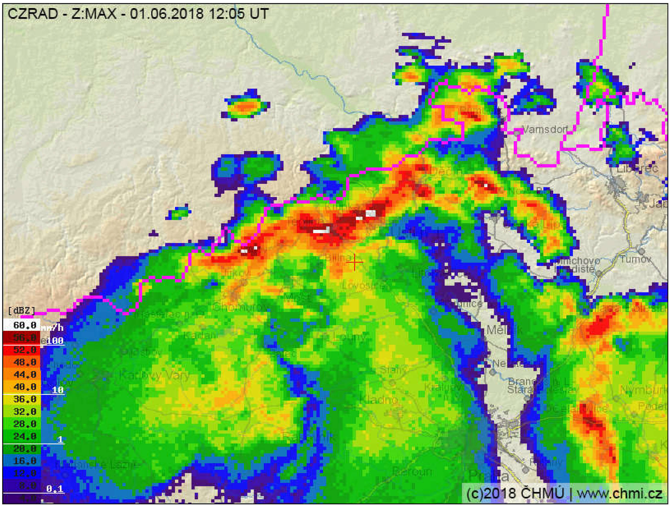
On 1 June 2018, a severe thunderstorm associated with precipitation and intense lightning occurred at the Milešovka observatory and its vicinity approximately between 12:00 and 12:30 UTC. Based on the information of the observer, the thunderstorm was related to a convective cell centered in the north of the observatory. Figure 2 shows the radar reflectivity that was measured by a C-band weather radar located 100 km southward from the Milešovka Mountain (Mt.) and operated by the Czech Hydrometeorological Institute.

The main precipitation cores (rain rates higher than 100 mm/h) were observed to be several kilometers in the North of the Milešovka Mt. (Figure 2). However, the one-minute precipitation maximum reached 1.5 mm at the Milešovka Mt., according to the rain gauge measurements (Figure 3).

In addition, a strong lightning activity was observed during the event with most of the lightning detected several kilometers in the north of the Milešovka Mt. (not depicted). Nevertheless, a thunder struck straight at the Milešovka observatory at approximately 12:10 UTC, according to the observer. The thunder stroke caused a power failure at the station even though the cloud radar measured unceasingly due to an uninterruptible power supply. The lightning, which directly strikes the observatory, is registered only once per year on average, which is one of the reasons for studying this particular event. Moreover, we selected this event because, since 1 June 2018, there were very few precipitation cases that were observed close to the observatory due to an unusually dry and sunny summer in the Czech Republic. None of these cases were related to strong lightning activity (as on 1 June 2018). The selected storm on 1 June 2018 is also considered significant in the context of the northwestern part of the Czech Republic because events with similar manifestations (e.g., occurrence of intense lightning) generally occurs only 10 times per year on average.

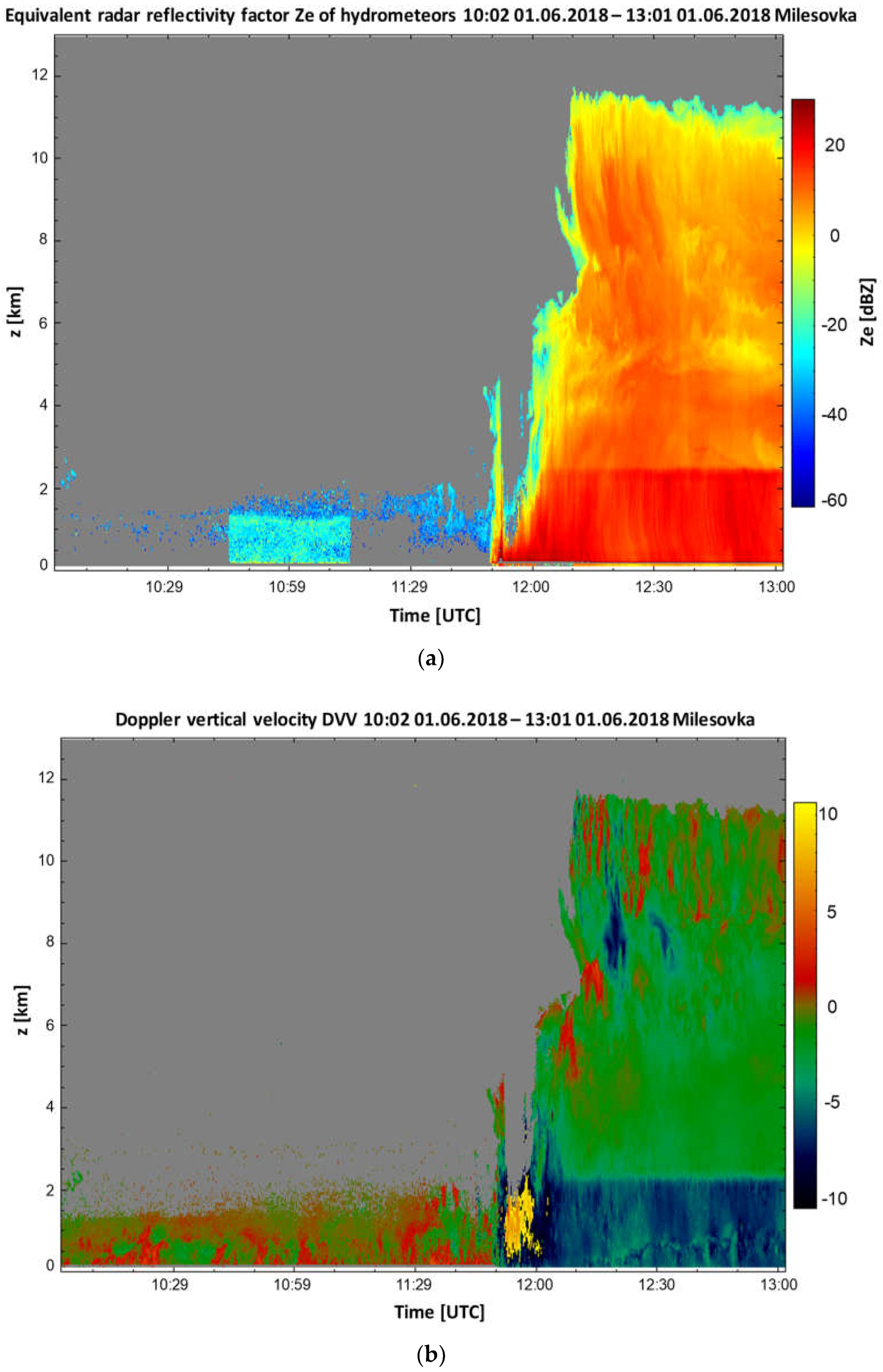
Figure 4 displays the standard products of IDLsoft during the thunderstorm on 1 June 2018 at the Milešovka observatory: the time evolution of (i) equivalent radar reflectivity (Figure 4a) and (ii) DVV oriented upward (Figure 4b). It follows from Figure 4 that the storm started moving across the Milešovka Mt. around 12:00 UTC. Figure 4b shows an aliasing in the DVV short before 12:00 UTC (yellow to dark yellow colors). Large negative DVV around 12:00 UTC indicate intense downdrafts in the radar position.

Table 2. Vertical temperature profile from sounding measurements at 12:00 UTC on 1 June 2018 based on the data from the Praha/Libuš station.

T [°C]	17.2	10	0	−10	−20
z [m]	0	842	2253	4278	5929

Note that z [m] corresponds to the height above the Milešovka Mt., which is situated at an elevation of 837 m a.s.l.

shows the vertical temperature profile during the event based on the aerological sounding measurements at 12:00 UTC from Praha/Libuš station (No. 11520). The aerological station is situated approximately 60 km from the Milešovka observatory.

2.4. Radar Data Processing

The cloud radar at the Milešovka Mt. processes measured data using the IDLsoft. The IDLsoft analyses Doppler spectra for each gate and determines at most 15 peaks in the Doppler spectrum. It also determines discrete intervals of the Doppler spectrum (ID) that include one peak each (http://metek.de/product/mira-35c/). For each ID, quantities such as DVV are calculated.

The Doppler processing of the I-Q signal consists of the following steps:

• Range gate decomposition
• Phase correction
• Calculation of the Fourier transform of the signal for each range gate
• Non-coherent averaging of the Doppler spectra
• Calculation of the noise level by applying the Hildebrand-Sekhon-Div algorithm based on Reference [30]
• Estimation of the three first moments, i.e., radar reflectivity, DVV, and spectrum width
• Estimation of derived quantities: Signal-to-Noise Ratio, equivalent radar reflectivity, and LDR

We used the measured data to retrieve the vertical air velocity (Section 2.5) and to classify the hydrometeors (Section 2.6).

2.5. Calculation of Vertical Air Velocity (Vair)

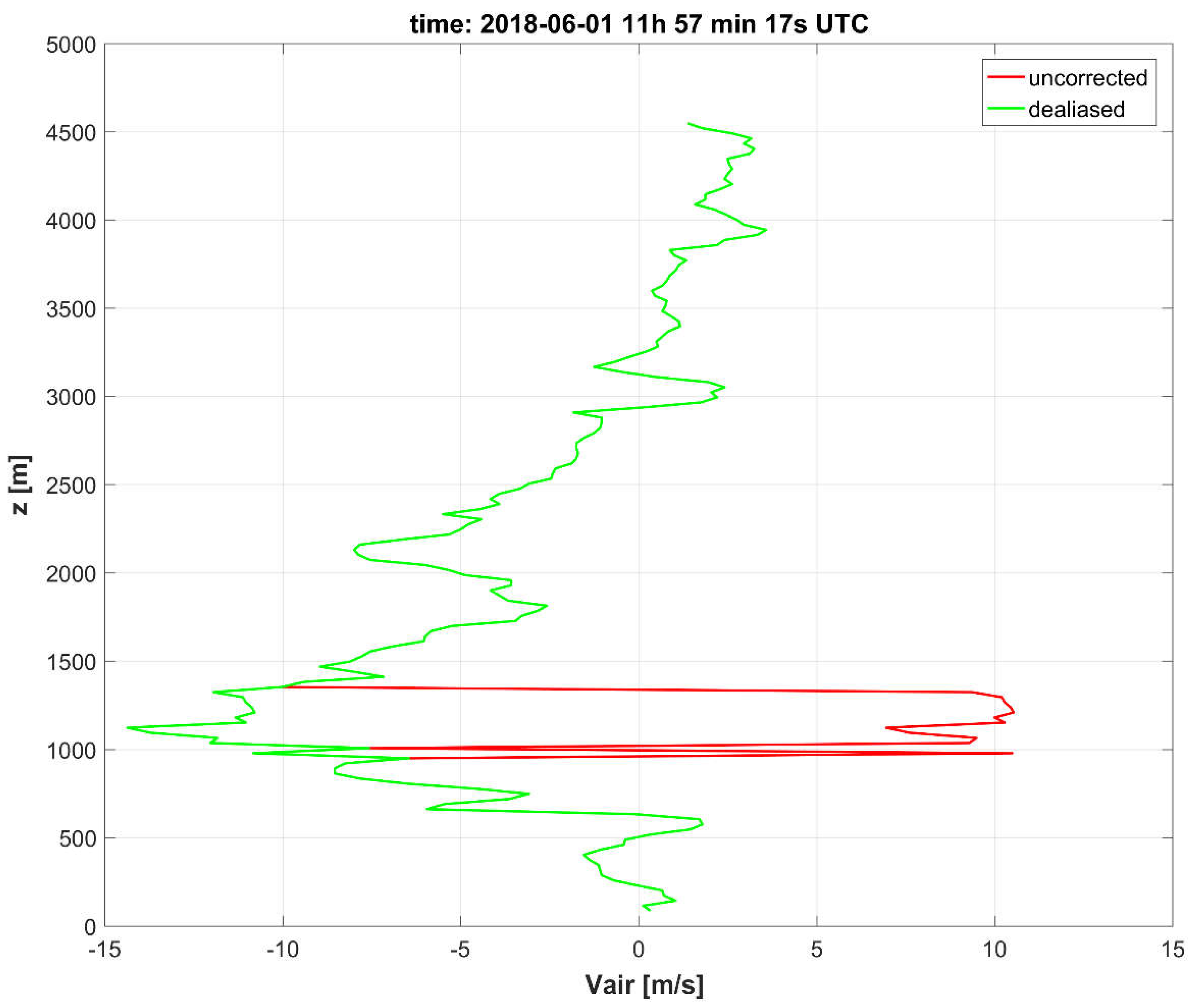
The calculation of vertical air velocity (Vair) is based on a known idea referred to a “small-particle-traced idea” in the literature. The small-particle-traced idea was described in References [9,10,31] and applied in Reference [6]. Our algorithm for retrieving the vertical air velocity from cloud radar measurements stems mostly from Reference [6]. Contrary to Reference [6], we developed a simple dealiasing algorithm for our vertically oriented radar. The dealiasing algorithm supposes that the velocity in the lowest gate is correct. The velocity in the next (upper) gate is checked and eventually corrected by using the condition that the difference in velocities in neighboring gates either does not exceed +10.65 m/s or is not lower than −10.65 m/s (see Table 1). An example of the dealiasing algorithm is given in Figure 5 where the vertical velocity is oriented downward towards the radar. The same (i.e., downward) orientation of the vertical velocity is used hereafter.

The small-particle-traced idea is based on a supposition that the cloud droplets and small particles of ice or snow have negligible terminal velocity. Therefore, their vertical velocity corresponds to that of the air motion. If the orientation of vertical velocity is downward towards the radar (as in Figure 5 and hereafter), then the terminal velocity is always positive and the velocity of small particles (e.g., cloud droplets) can be estimated from the Doppler spectrum for vertically pointing radar based on known variances induced by (i) particle size distribution, (ii) turbulence, (iii) wind shear, and (iv) finite radar beam width [6].

In our study, we estimated Vair based on the procedure applied in Reference [6] with two modifications. The first modification that we required is that the amplitude of the left edge of the Doppler spectra is at least 0.1% of the maximum amplitude of Doppler spectra for any given measurement. This modification was motivated by the results of our tests, which revealed an insufficient removal of noise by S_TH (see Section 2.1). Specifically, Doppler spectra with a very low amplitude were not removed by S_TH. Therefore, the left edge of the Doppler spectra was giving unrealistic vertical velocities or velocities inconsistent with the velocities in neighboring gates.

The value of 0.1% is based on the testing of various S_TH ranging from 0.0001% to 1% of the maximum amplitude of Doppler spectra and on the evaluation of maximum differences in Vair between neighboring gates. The gates are above and below the evaluated gate. While the differences in Vair were large for S_TH = 0.05% and lower, the differences were significantly smaller for the S_TH ranging from 0.1% to 1%. Therefore, we considered 0.1% of the maximum amplitude of Doppler spectra as a suitable value of S_TH for our algorithm for any given measurement. It should be noted that we suppose the existence of “small-particles” even if they are not later recognized by the classification algorithm of hydrometeors (Section 2.6).

The second modification was related to horizontal wind shear calculations since our cloud radar is vertically oriented. We defined the horizontal wind shear df/dx by assuming that the horizontal wind does not change along the Lagrangian trajectories.

df/dx = −(1/u)(u(t) − u(t-dt))/dt,

(1)

where u is the horizontal wind velocity [m/s] measured by an aerological balloon at a time t while dt [s] is the time resolution of radar measurements (i.e., 2 s approximately).

2.6. Classification of Hydrometeors

The algorithm that we applied to classify hydrometeors stems from the assumption that the terminal velocity of various hydrometeors differs. Note that the terminal velocity of a hydrometeor might suggest whether the hydrometeor falls to the ground, i.e., becomes precipitation (rain, hail etc.), or it evaporates before reaching the ground depending on the air temperature. Thus, we also suppose in our algorithm that the occurrence of single hydrometeor depends on air temperature and partially on LDR, which indicates the shape of hydrometeors.

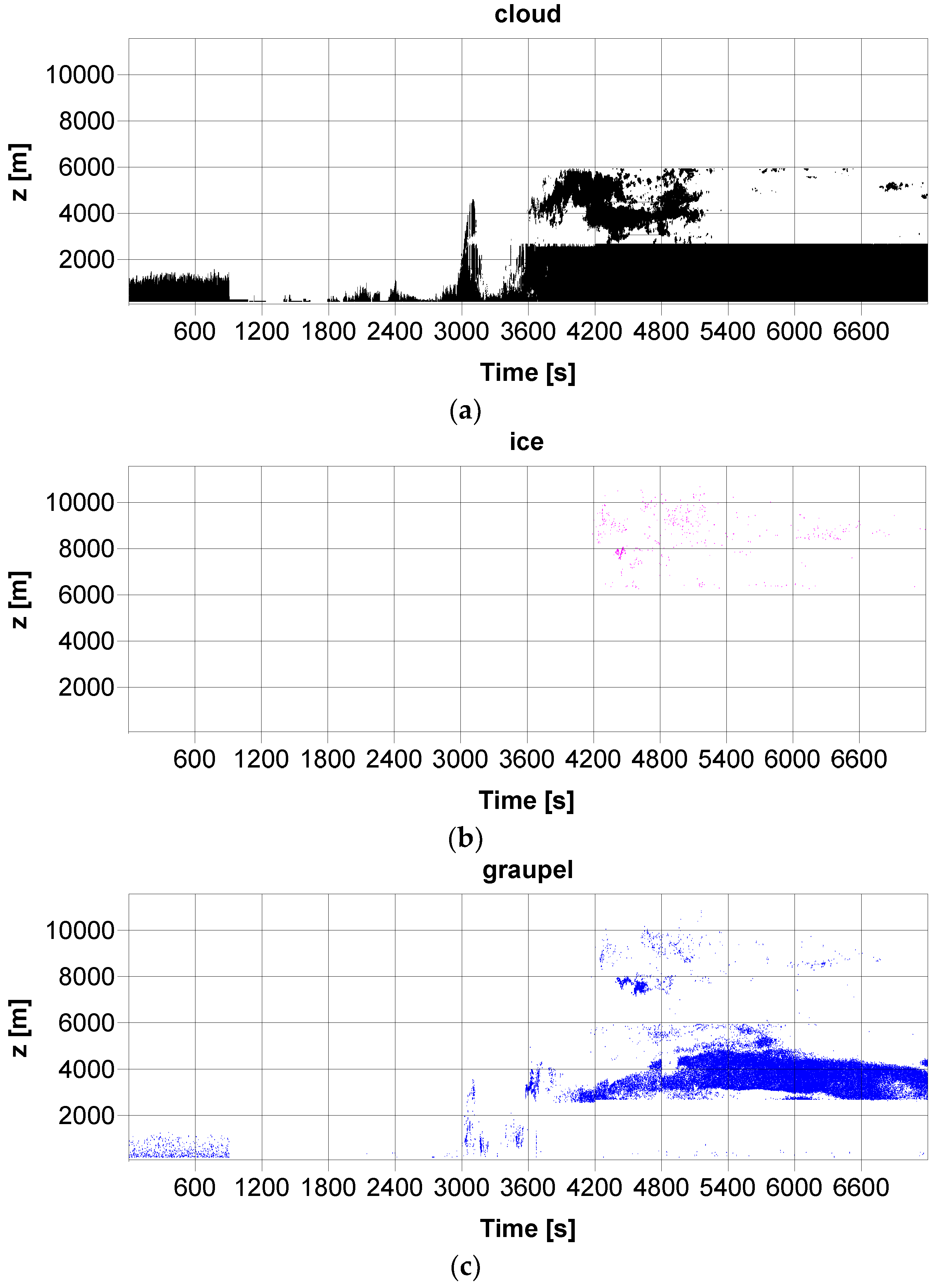
We used six types of hydrometeors: cloud, graupel, ice, snow, rain, and hail. Cloud droplets and small ice crystals are usually non-precipitating hydrometeors while rain, graupel, snow, and hail represent hydrometeors that can also be detected at the ground as precipitation. The interval of terminal velocity of a hydrometeor was derived from parameters of hydrometeors considered in the COSMO numerical weather prediction model. We selected the parameter values that belong to “standard” hydrometeors and that we use whenever we run the COSMO e.g., Reference [32]. Note that, in this study, we did not make any simulation in COSMO. We only took the parameter values of the six hydrometeors from COSMO. We slightly modified the original intervals of terminal velocity to avoid intersections within both the liquid and the solid hydrometeors (i.e., to get discrete intervals).

Table 3. Six types of hydrometeors and their minimum and maximum terminal velocity [m/s] (Vmin and Vmax, respectively) and minimum and maximum air temperature [°C] (Tmin and Tmax, respectively) within which the hydrometeors may occur.

Hydrometeor	Vmin [m/s]	Vmax [m/s]	Tmin [°C]	Tmax [°C]
Cloud	0.0001	0.1543	−20	40
Rain	0.1543	6.3384	−20	40
Snow	0.0290	1.2458	−70	0
Ice	1.2458	1.3133	−70	0
Graupel	1.3133	7.7747	−70	40
Hail	7.7747	10.0253	−70	40

shows the six types of hydrometeors that we retrieve. It displays minimum terminal velocity of individual hydrometeors (Vmin), maximum terminal velocity of individual hydrometeors (Vmax), and temperature intervals at which the individual hydrometeors can occur.

The classification is performed for each gate on a condition that at least one ID is found. It should be noted that DVV (Figure 4b) is the weighted average of the spectrum of measured Doppler velocities (i.e., spectrum components) with the weight corresponding to the measured reflectivity of individual spectrum components. As a rule, the spectrum contains several peaks, which can significantly differ in corresponding speeds. Thus, they may correspond to different hydrometeors. The peaks and surrounding ID are determined by the IDLsoft during the basic processing of measured data.

The hydrometeor classification algorithm is performed for each peak and consists of two preliminary steps:

• Calculation of vertical temperature profile: We use aerological sounding measurements of temperature from station Praha/Libuš, which are linearly interpolated in time and height above the ground. The station is located 60 km southward from the Milešovka Mt. The measurements are regularly provided at 00, 06, and 12 UTC. Since we do not perform the classification of hydrometeors in real time, it is possible to interpolate the measurements in time.
• Computation of terminal velocity (Vter): terminal velocity is determined for each ID by subtracting Vair from the Doppler velocity for the given peak (DVP).

Vter(ID) = DVP − Vair.

(2)

Since it is well known that the occurrence of hydrometeors depends on air temperature T, we considered three temperature intervals in our study. We suppose that, below −20 °C, the water is fully frozen and therefore graupel, ice, snow, and hail can occur while cloud and rain droplets cannot occur. When the temperature is above 0 °C, we assume that cloud and rain droplets, graupel, and hail can appear while ice and snow cannot. In between (i.e., from −20 °C to 0 °C) in convective storms, it is assumed that solid hydrometeors occur while liquid hydrometeors can occur only in the case when the air rises up (Vair ≤ −0.01 m/s in the code) because, in this case, the cloud droplets are vertically advected. They do not freeze immediately and, instead, they become supercooled.

Based on Vter, Vmax, and Vmin (Table 3), Vair, and LDR, we define the hydrometeors in the three temperature intervals below.

• T < −20 °C
  • If Vter < Vmin(ice), then the hydrometeor is classified as snow.
  • If Vmin(ice) ≤ Vter < Vmax(ice), then the hydrometeor is classified as ice.
  • If Vmin(graupel) ≤ Vter < Vmax(graupel), then the hydrometeor is classified as graupel.
  • If Vter ≥ Vmax(graupel), then the hydrometeor is classified as hail.
• T > 0 °C
  • If Vter < Vmax(cloud), then the hydrometeor is classified as a cloud droplet.
  • If Vmin(rain) ≤ Vter < Vmin(graupel), then the hydrometeor is classified as rain.
  • If Vmin(graupel) ≤ Vter < Vmax(rain) and LDR < 0.05, then the hydrometeor is classified as rain. Otherwise, it is classified as graupel.
  • If Vmax(rain) ≤ Vter < Vmax(graupel), then the hydrometeor is classified as graupel.
  • If Vter ≥ Vmax(graupel), then the hydrometeor is classified as hail.
• −20 °C ≤ T ≤ 0 °C
  • If Vair ≤ −0.01 m/s and Vter < Vmax(cloud), then two types of hydrometeors are supposed to occur: cloud droplet and snow.
  • If Vair > −0.01 m/s and Vter < Vmax(cloud), then the hydrometeor is classified as snow even if Vter < Vmin(snow).
  • If Vmax(cloud) ≤ Vter < Vmax(snow), then the hydrometeor is classified as snow.
  • If Vmin(ice) ≤ Vter < Vmax(ice), then the hydrometeor is classified as ice.
  • If Vmin(graupel) ≤ Vter < Vmax(graupel), then the hydrometeor is classified as graupel.
  • If Vter ≥ Vmax(graupel), then the hydrometeor is classified as hail.

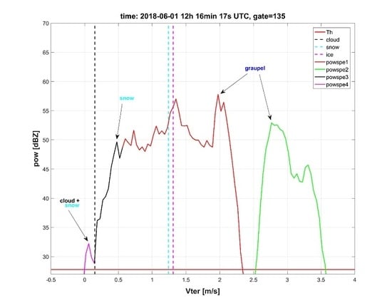
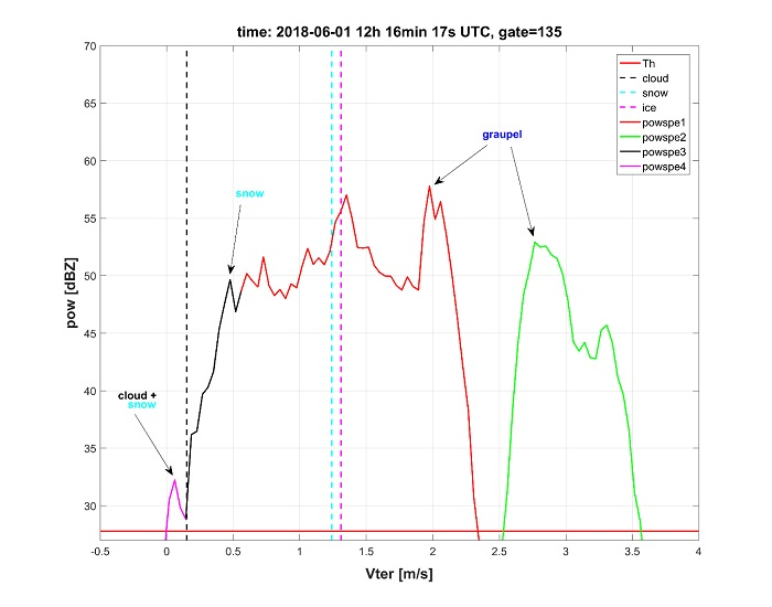
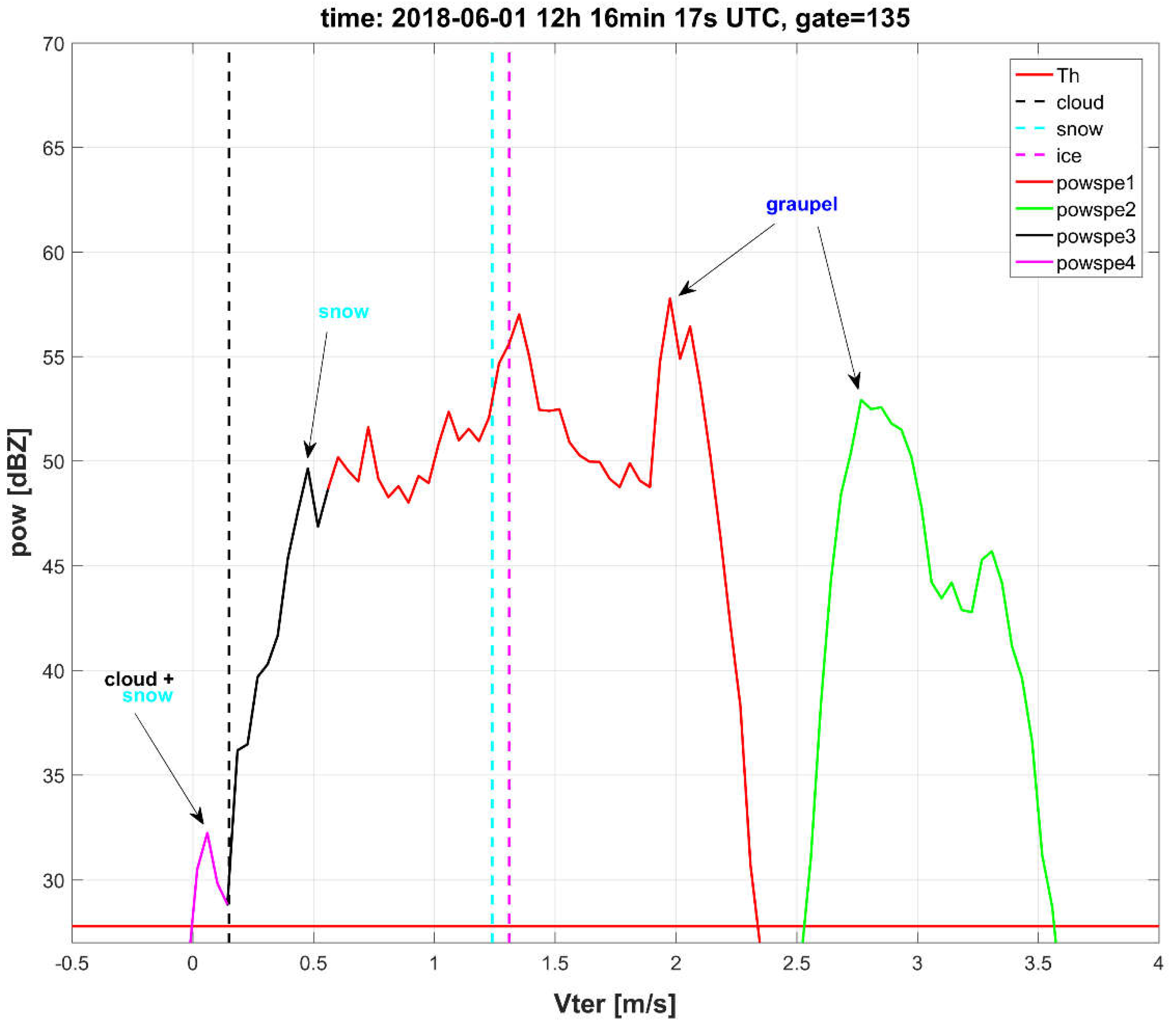
Figure 6 shows an example of the hydrometeor classification on 1 June 2018 for a gate situated 4059 m above the radar. It shows the power spectrum corrected by Vair (Section 2.5). The peaks of the power spectrum and corresponding ID are determined by the IDLsoft and the hydrometeor classification is performed by using our algorithm following the above given rules.

3. Results

This section displays and comments the results of Vair that we computed during the studied thunderstorm on 1 June 2018 (Section 3.1). It also describes and evaluates the identified hydrometeor classes during the event (Section 3.2).

3.1. Vair during the Thunderstorm on 1 June 2018

Time development of Vair (calculated according to Section 2.5) during the thunderstorm on 1 June 2018 is displayed in Figure 7. Figure 7 also compares the calculated Vair to DVV during the thunderstorm. It is obvious from Figure 7 that the DVV is generally higher than Vair. The higher values of DVV are expected since DVV corresponds to the sum of Vair and terminal velocity (Vter) where Vter is always positive due to the downward orientation of the vertical velocity and the downward movement of hydrometeors.

We cannot explicitly verify the correctness of the derived values of Vair because we do not have any other available measurements to which we could compare our results. Therefore, we subjectively evaluated the results by using the general knowledge of the structure of vertical motion in storms. The obtained distribution of the derived vertical velocities mostly correspond to our expectations. Negative Vair is visible in the heights from 3 to almost 12 km prior to and during the observed maximum storm activity at the Milešovka Mt. (from 12:00 to 12:20 UTC). Regions with a significant negative Vair are obvious in heights from 6 to 8 km from 12:00 to 12:20 UTC, which corresponds to the layer of usually observed negative Vair minima in storms. Noticeable negative Vair values in the heights of around 10 km are less typical in storms even though they also appear in Figure 7.

It should be noted that the minimum gate values of Vair were lower than −10 m/s in only several individual points in Figure 7a and, thus, they are not very noticeable in the Figure 7a. On the contrary, velocities lower than −5 m/s are clearly visible in quite large areas in Figure 7a. While at the beginning of the storm, i.e., around 12:00 UTC, negative values of Vair dominate the middle troposphere while after 12:30 UTC approximately Vair evinces mainly positive values in the low and middle troposphere. The positive values of Vair in the low and middle troposphere are typical for the mature and dissipation stage of storms.

One should be aware, while evaluating the values of Vair, that the vertically oriented cloud radar does not show any cross-section of the evolving storm, which the trajectory may significantly differ from a straight line. Thus, the results cannot be directly compared with drawings of conceptual models of storms. Moreover, the measured event consisted of several connected convective cores, which developed in time and moved in space (Figure 2). It means that, despite the uncertainty related to Vair, we do not have any means in our disposal to objectively verify the resulting Vair. However, we are convinced that the derived Vair has a physical justification and, therefore, can be used in further computations.

Concerning values of DVV given by the IDLsoft (Figure 4b), one can observe that our algorithm successfully applies the dealiasing algorithm, which removes the majority of unrealistic values of DVV that are most apparent before 12:00 UTC (i.e., 3600 s in Figure 7b). At that time, the IDLsoft shows a sharp difference of DVV from less than −10 m/s to more than +10 m/s (Figure 4b), which is very unlikely. Note that the DVV in Figure 7b differs from DVV in Figure 4b, produced by IDLsoft, by subtracting Vair, and the DVV in Figure 4b is of the opposite sign than DVV in Figure 7b due to the upward and downward orientation of vertical velocity, respectively.

3.2. Hydrometeors during the Thunderstorm on 1 June 2018

The classification of hydrometeors (Section 2.6) provides a distribution of hydrometeors in clouds. Figure 8 depicts the distribution of the six considered hydrometeors in the thundercloud during the thunderstorm on 1 June 2018 at the Milešovka Mt. Note that more than one hydrometeor can be detected at a point (as shown in Figure 6). The hydrometeors are allowed to overlap if they follow the conditions given in Section 2.6.

Figure 8 displays that precipitation in the form of rain, graupel, and hail are detected at the ground level by the algorithm. Figure 8a shows that cloud droplets are highly concentrated in lower layers up to approximately 2500 m above the Milešovka Mt., which is the altitude that roughly matches with the melting layer (i.e., bright band in Figure 4a, Table 2). The cloud droplets observed in higher altitudes correspond to the super-cooled droplets that can be observed above the melting layer in thunderclouds.

Contrary to cloud droplets, snow particles (Figure 8f) show the highest concentrations above the melting layer. Snow particles were the most dominant hydrometeor type during the study event on 1 June 2018. On the other hand, ice particles (Figure 8b) were identified the least often during the event by our algorithm due to the fact that the interval of terminal velocities is much smaller for ice than that for snow (Table 3). For our investigation, it is not crucial to distinguish between snow and ice. Therefore, we consider a fusion of the two particles in one hydrometeor type in the future. However, we plan to test the current algorithm on more events first.

Graupel (Figure 8c) was mostly concentrated above the melting layer (2500–4500 m) while rain (Figure 8d) was mainly located in the melting layer or below. Our algorithm also identified hail in the layer of up to 2 km primarily around 12:00 UTC (Figure 8e). However, the occurrence of hail at approximately 12:00 UTC was not confirmed by the observer at the ground.

4. Discussion

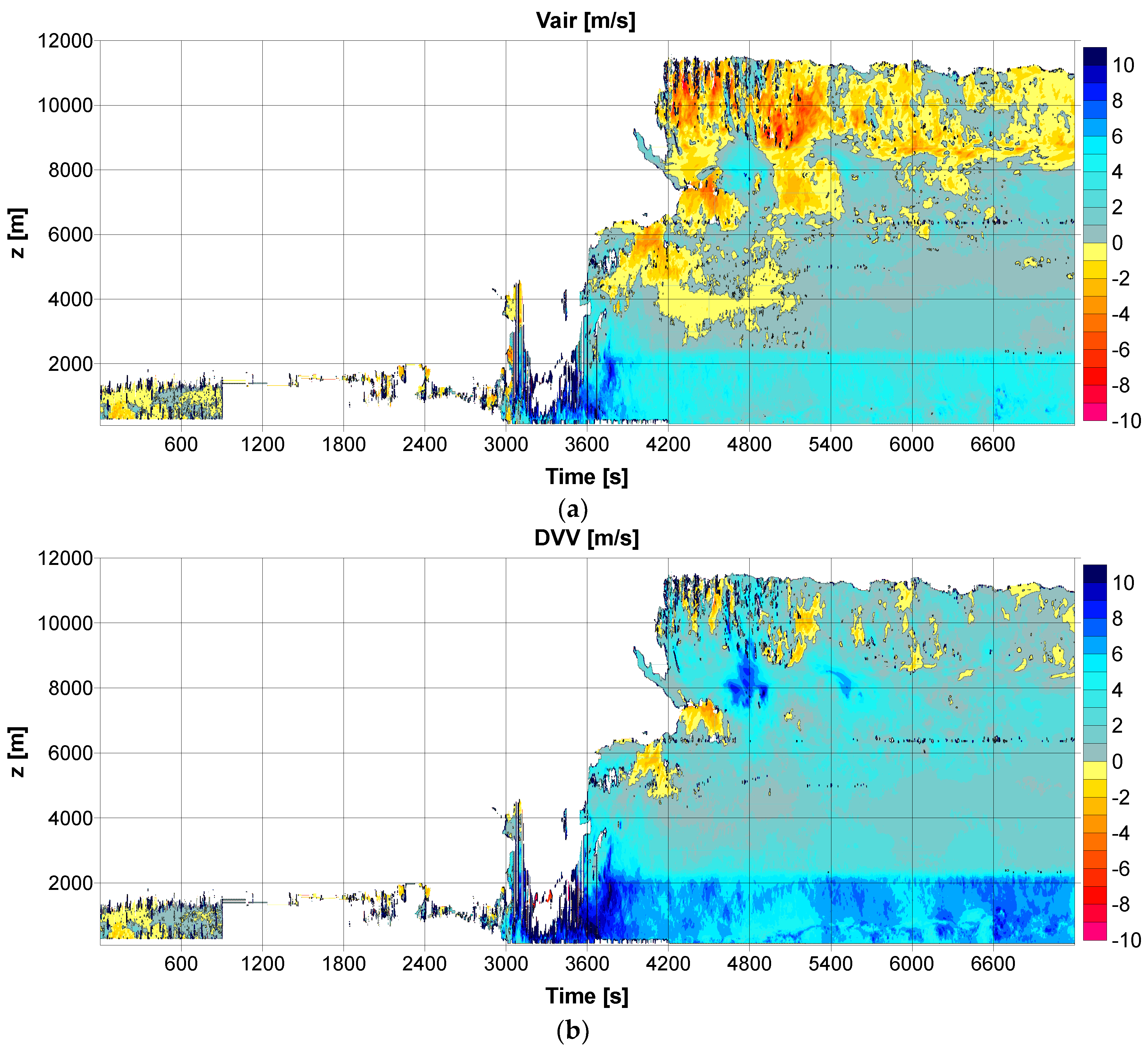
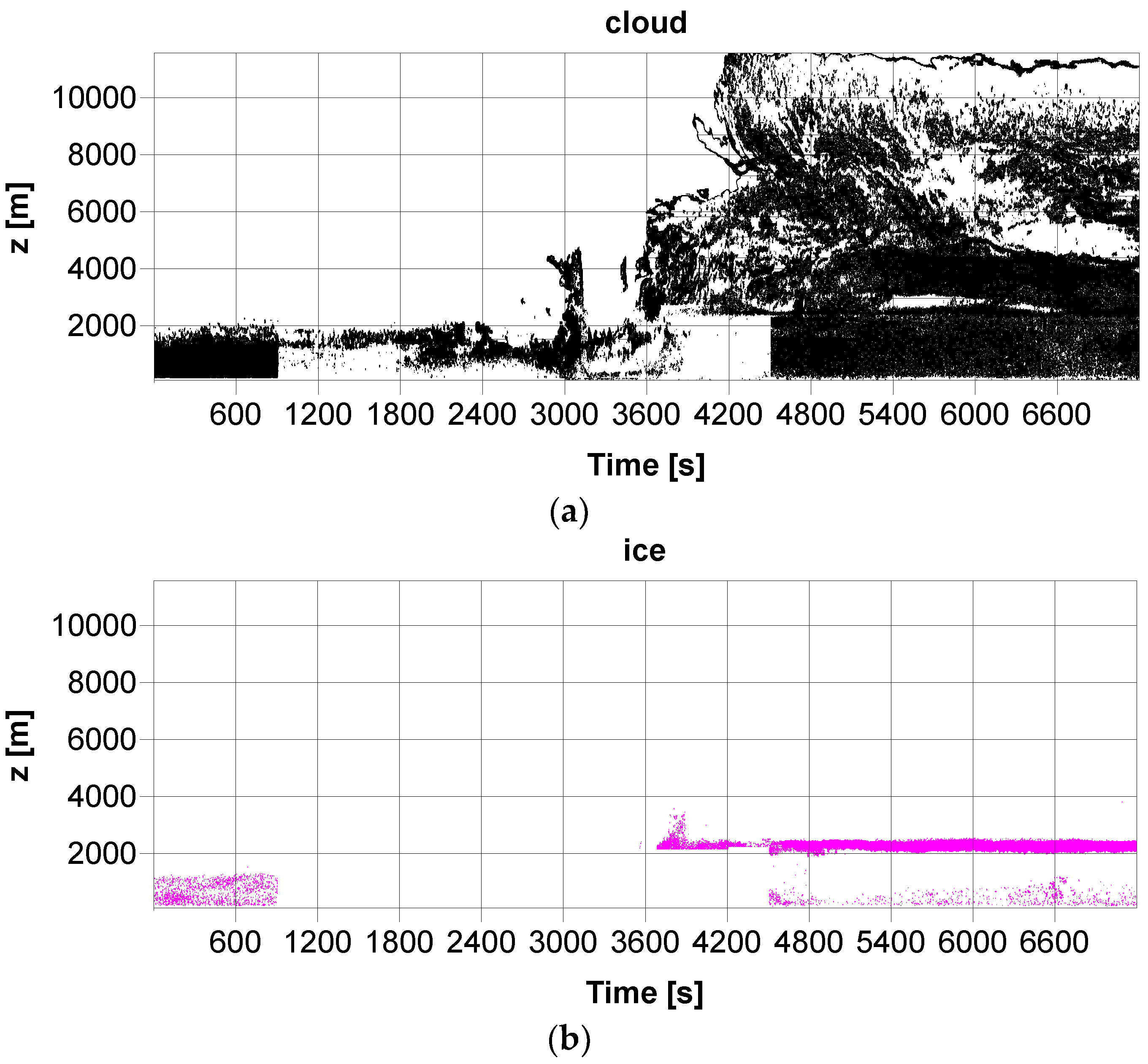
We compared the results of the distribution of hydrometeors during the studied thunderstorm by our algorithm (Figure 8) with the results given by the provider of the cloud radar, i.e., the IDLsoft. The IDLsoft recognizes three types of hydrometeors based on Reference [29], which includes cloud, ice, and rain. Rain includes any kind of precipitation that has a significant fall velocity such as graupel or hail and can fall to the ground [29].

Figure 9 displays the distribution of the three hydrometeors identified by the IDLsoft during the thunderstorm on 1 June 2018. It shows that both ice and rain particles reached the ground level (i.e., precipitated), according to the IDLsoft. Moreover, the IDLsoft identified ice particles mainly in the melting layer and raindrops at the altitude of up to 12 km (Figure 9). As we mentioned above, in the IDLsoft rain is a precipitation that includes all particles (liquid and/or solid) with high terminal velocity while ice and cloud hydrometeors represent particles with small terminal velocities in the IDLsoft. However, a clear condition dividing particles between the cloud and the ice is not mentioned in Reference [29]. We expect that cloud particles represent solid particles in higher altitudes (i.e., snow and/or ice), which is similar to rain and includes solid particles in higher altitudes (graupel and/or hail). A personal communication with M. Bauer-Pfundstein pointed out that their algorithm might not be necessarily valid during thunderstorms.

As a result, we can assume that, although simple, our algorithm provides satisfying and plausible distribution of hydrometeors during thunderstorms (e.g., Figure 8) and the algorithm can be considered a suitable extension to the existing IDLsoft. However, further testing and verification of the algorithm are needed.

As far as LDR values are concerned, the use of it is rather marginal in our classification of hydrometeors. The analysis of the studied thunderstorm and of few clouds detected by the radar since June 2018 showed that the LDR values are usually available up to the height of the melting layer approximately. At higher altitudes, the LDR data are often unavailable due to strong attenuation of the signal. Therefore, we cannot base the hydrometeor classification on LDR values. In addition, for a vertically pointing radar, a slanted radar antenna (for instance 20°) might be more appropriate for the efficient use of LDR to classify the cloud particles. In any case, the use of LDR in the hydrometeor classification will be addressed in further research.

In the future, we will test the algorithm by using more thunderstorm events, which was not possible in this study due to an unusually dry and sunny summer in the Czech Republic (i.e., no similar thunderstorm has been detected at the station since the analyzed 1 June 2018). We will compare the results using six hydrometeor types to that using five hydrometeor types (ice and snow as one hydrometeor type). Moreover, we plan to compare the derived variables from the cloud radar with that of other instruments, e.g., disdrometer and ceilometer, situated at the Milešovka observatory.

5. Conclusions

The study presented two new functionalities that complement the provided software of a vertically pointing Ka-band cloud radar, which was located at the Milešovka observatory in Central Europe in 2018. The radar has been installed in order to study the cloud structure including thunderclouds. We improved the dealiasing algorithm and we applied a method for computing the vertical air velocity and the terminal velocity of hydrometeors by using the Doppler spectra. We developed an algorithm that enables one to classify the hydrometeors that can lead to precipitation. We illustrated the algorithms with a thunderstorm that crossed the Milešovka observatory on 1 June 2018 and was associated with significant lightning activity.

The method retrieving vertical air velocity, which is a variable needed for our classification of hydrometeors, was subjectively evaluated because we have no means to perform any objective verification. In our opinion, the obtained distribution of vertical air velocity in time and height is in good agreement with the structure of air velocity expected in storms and, therefore, we used the retrieved vertical air velocity in the algorithm classifying hydrometeors.

The algorithm classifying hydrometeors uses the information on vertical air velocity, temperature from sounding measurements from the nearest aerological station, terminal velocity, and LDR in non-precipitating/precipitating clouds. The resulting distribution of six considered hydrometeors (cloud droplets, ice and snow particles, rain, graupel, and hail) seems realistic for the thunderstorm on 1 June 2018 and more plausible than that obtained from the provided radar products for the thunderstorm. Nevertheless, the results pointed out that the method hardly distinguishes snow from ice and vice versa.