Mapping and Forecasting Onsets of Harmful Algal Blooms Using MODIS Data over Coastal Waters Surrounding Charlotte County, Florida


Abstract
1. Introduction
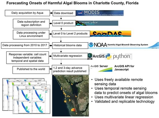
2. Materials and Methods
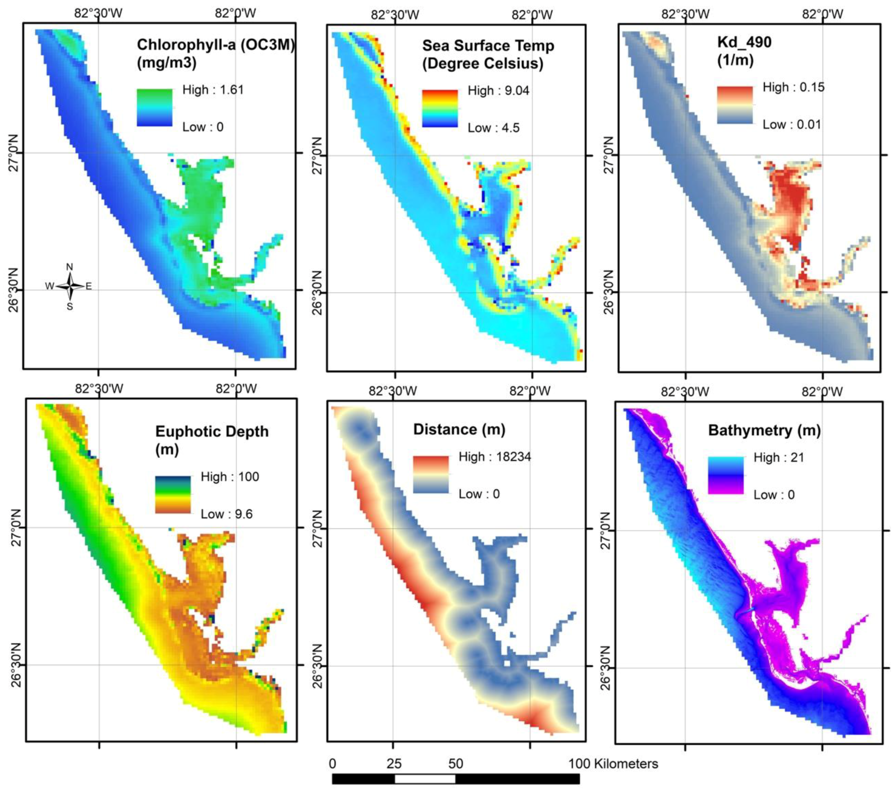
2.1. Step 1
2.1.1. Euphotic Depth (m)
2.1.2. Wind Direction (Degrees) and Wind Speed (m/s)
2.1.3. Chlorophyll-a (mg/m3)
2.1.4. Diffuse Attenuation Coefficient
2.1.5. Turbidity Index
2.1.6. Particulate Backscattering Coefficient at 547 nm
2.1.7. Sea Surface Temperature (°C)
2.1.8. Fluorescence Line Height (FLH)
2.1.9. Bathymetry (m)
2.1.10. Distance from the River Mouth (m)
2.2. Step 2
2.3. Step 3
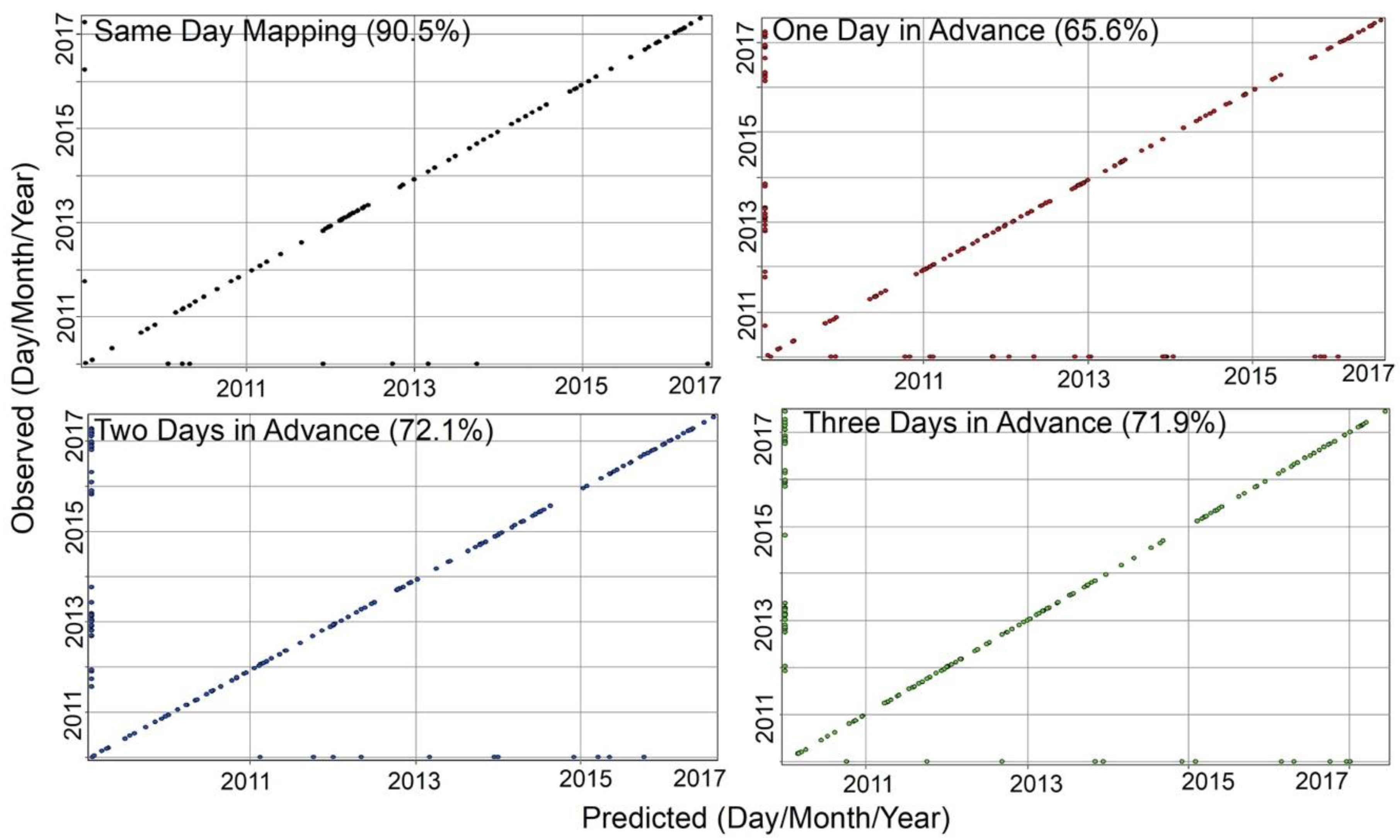
3. Results
4. Discussion
5. Conclusions
Author Contributions
Funding
Acknowledgments
Conflicts of Interest
References
- Glibert, P.M.; Harrison, J.; Heil, C.; Seitzinger, S. Escalating worldwide use of urea—A global change contributing to coastal eutrophication. Biogeochemistry 2006, 77, 441–463. [Google Scholar] [CrossRef]
- Howarth, R.W.; Billen, G.; Swaney, D.; Townsend, A.; Jaworski, N.; Lajtha, K.; Downing, J.A.; Elmgren, R.; Caraco, N.; Jordan, T.; et al. Regional nitrogen budgets and riverine inputs of N and P for the drainages to the North Atlantic Ocean: Natural and human influences. Biogeochemistry 1996, 35, 75–139. [Google Scholar] [CrossRef]
- Landsberg, J.H. The effects of harmful algal blooms on aquatic organisms. Rev. Fish. Sci. Aquac. 2002, 10, 113–390. [Google Scholar] [CrossRef]
- Fleming, L.E.; Kirkpatrick, B.; Backer, L.C.; Walsh, C.J.; Nierenberg, K.; Clark, J.; Reich, A.; Hollenbeck, J.; Benson, J.; Cheng, Y.S.; et al. Review of Florida red tide and human health effects. Harmful Algae 2011, 10, 224–233. [Google Scholar] [CrossRef] [PubMed]
- Steidinger, K.A.; Vargo, G.A.; Tester, P.A.; Tomas, C.R. Bloom dynamics and physiology of Gymnodinium breve with emphasis on the Gulf of Mexico. In Physiological Ecology of Harmful Algal Blooms, 1st ed.; Anderson, D.M., Cambella, A.D., Hallegraeff, G.M., Eds.; Springer: Heidelberg, Germany, 1998; pp. 133–154. ISBN 3540641173. [Google Scholar]
- Amin, R.; Zhou, J.; Gilerson, A.; Gross, B.; Moshart, F.; Ahmed, S. Novel optical techniques for detecting and classifying toxic dinoflagellate Karenia brevis blooms using satellite imagery. Opt. Express 2009, 17, 9126–9144. [Google Scholar] [CrossRef] [PubMed]
- Thyng, K.M.; Hetland, R.D.; Ogle, M.T.; Zhang, X.; Chen, F.; Campbell, L. Origins of Karenia brevis harmful algal blooms along the Texas coast. Limnol. Oceanogr. Fluids Environ. 2013, 3, 269–278. [Google Scholar] [CrossRef]
- Evans, G.; Jones, L. Economic Impact of the 2000 Red Tide on Galveston County; A Case Study: Austin, TX, USA, 2001. [Google Scholar]
- Raine, R.; McDermott, G.; Silke, J.; Lyons, K.; Nolan, G.; Cusack, C. A simple short range model for the prediction of harmful algal events in the bays of southwestern Ireland. J. Mar. Syst. 2010, 83, 150–157. [Google Scholar] [CrossRef]
- Cha, Y.; Park, S.S.; Kim, K.; Byeon, M.; Stow, C.A. Probabilistic prediction of cyanobacteria abundance in a Korean reservoir using a Bayesian Poisson model. Water Resour. Res. 2014, 50, 2518–2532. [Google Scholar] [CrossRef]
- Harred, L.B.; Campbell, L. Predicting harmful algal blooms: A case study with Dinophysis ovum in the Gulf of Mexico. J. Plankton Res. 2014, 36, 1434–1445. [Google Scholar] [CrossRef]
- McGillicuddy, D.J.; Anderson, D.M.; Lynch, D.R.; Townsend, D.W. Mechanisms regulating large-scale seasonal fluctuations in Alexandrium fundyense populations in the Gulf of Maine: Results from a physical-biological model. Deep Sea Res. Part II Top. Stud. Oceanogr. 2005, 52, 2698–2714. [Google Scholar] [CrossRef]
- Cusack, C.; Dabrowski, T.; Lyons, K.; Berry, A.; Westbrook, G.; Salas, R.; Duffy, C.; Nolan, G.; Silke, J. Harmful Algal Bloom forecast system for SW Ireland. Part II: Are operational oceanographic models useful in a HAB warning system? Harmful Algae 2016, 53, 86–101. [Google Scholar] [CrossRef] [PubMed]
- Aleynik, D.; Dale, A.C.; Porter, M.; Davidson, K. A high resolution hydrodynamic model system suitable for novel harmful algal bloom modelling in areas of complex coastline and topography. Harmful Algae 2016, 53, 102–117. [Google Scholar] [CrossRef] [PubMed]
- Gillibrand, P.A.; Siemering, B.; Miller, P.I.; Davidson, K. Individual-based modelling of the development and transport of a Karenia mikimotoi bloom on the North-West European continental shelf. Harmful Algae 2016, 53, 118–134. [Google Scholar] [CrossRef] [PubMed]
- Stumpf, R.P.; Litaker, R.W.; Lanerolle, L.; Tester, P.A. Hydrodynamic accumulation of Karenia off the West Coast of Florida. Cont. Shelf Res. 2008, 28, 189–213. [Google Scholar] [CrossRef]
- Turrell, E.; Stobo, L.; Lacaze, J.P.; Bresnan, E.; Gowland, D. Development of an ‘early warning system’ for harmful algal blooms using solid-phase adsorption toxin tracking (SPATT). In Proceedings of the OCEANS 2007—Europe, Aberdeen, UK, 18–21 June 2007; pp. 1–6. [Google Scholar] [CrossRef]
- Lee, J.H.W.; Hodgkiss, I.J.; Wong, K.T.M.; Lam, I.H.Y. Real time observations of coastal algal blooms by an early warning system. Estuar. Coast Shelf Sci. 2005, 65, 172–190. [Google Scholar] [CrossRef]
- Hu, C.; Muller-Karger, F.E.; Taylor, C.; Carder, K.L.; Kelble, C.; Johns, E.; Heil, C.A. Red tide detection and tracing using MODIS fluorescence data: A regional example in SW Florida coastal waters. Remote Sens. Environ. 2005, 97, 311–321. [Google Scholar] [CrossRef]
- Carvalho, G.A.; Minnett, P.J.; Fleming, L.E.; Banzon, V.F.; Baringer, W. Satellite remote sensing of harmful algal blooms: A new multi-algorithm method for detecting the Florida Red Tide (Karenia brevis). Harmful Algae 2010, 9, 440–448. [Google Scholar] [CrossRef] [PubMed]
- Al Shehhi, M.R.; Gherboudj, I.; Zhao, J.; Mezhoud, N.; Ghedira, H. Evaluating the performance of MODIS FLH ocean color algorithm in detecting the Harmful Algae Blooms in the Arabian Gulf and the Gulf of Oman. In OCEANS 2013 MTS/IEEE—San Diego; An Ocean in Common: San Diego, CA, USA, 2013; pp. 1–7. [Google Scholar]
- Neville, R.A.; Gower, J.F.R. Passive remote sensing of phytoplankton via chlorophyll fluorescence. J. Geophys. Res. 1977, 82, 3487–3493. [Google Scholar] [CrossRef]
- Pan, D.L.; Gower, J.F.R.; Lin, S.R. A study of band selection for fluorescence remote sensing of ocean chlorophyll-a. Oceanol. Limnol. Sin. 1989, 20, 564–570. [Google Scholar]
- Fischer, J.; Kronfeld, U. Sun-stimulated chlorophyll fluorescence: 1. Influence of oceanic properties. Int. J. Remote Sens. 1990, 11, 2125–2147. [Google Scholar] [CrossRef]
- Hoge, F.E.; Lyon, P.E.; Swift, R.N.; Yungel, J.K.; Abbott, M.R.; Letelier, R.M.; Esaias, W.E. Validation of Terra-MODIS phytoplankton chlorophyll fluorescence line height. I. Initial airborne lidar results. Appl. Opt. 2003, 42, 2767–2771. [Google Scholar] [CrossRef] [PubMed]
- Balch, W.M.; Eppley, R.W.; Abbott, M.R.; Reid, F.M.H. Bias in satellite-derived pigment measurements due to coccolithophores and dinoflagellates. J. Plankton Res. 1989, 11, 575–581. [Google Scholar] [CrossRef]
- Stumpf, R.P.; Culver, M.E.; Tester, P.A.; Tomlinson, M.; Kirkpatric, G.J.; Pederson, B.A.; Truby, E.; Ransibrahmanakul, V.; Soracco, M. Monitoring Karenia brevis blooms in the Gulf of Mexico using satellite ocean color imagery and other data. Harmful Algae 2003, 2, 147–160. [Google Scholar] [CrossRef]
- Gower, J.F.R.; Brown, L.; Borstad, G.A. Observations of chlorophyll fluorescence in west coast waters of Canada using the MODIS satellite sensor. Can. J. Remote Sens. 2004, 30, 17–25. [Google Scholar] [CrossRef]
- Tomlinson, M.C.; Wynne, T.T.; Stumpf, R.P. An evaluation of remote sensing techniques for enhanced detection of the toxic dinoflagellate, Karenia Brevis. Remote Sens. Environ. 2009, 113, 598–609. [Google Scholar] [CrossRef]
- Zhao, D.Z.; Xing, X.G.; Liu, Y.G.; Yang, J.H.; Wang, L. The relationship of chlorophyll-a concentration with the reflectance peak near 700 nm in algae-dominated waters and sensitivity of fluorescence algorithms for detecting algal bloom. Int. J. Remote Sens. 2010, 31, 39–48. [Google Scholar] [CrossRef]
- Tang, D.L.; Ni, I.H.; Kester, D.R.; Müller-Karger, F.E. Remote sensing observation of winter phytoplankton blooms southwest of the Luzon Strait in the South China Sea. Mar. Ecol. Prog. Ser. 1999, 191, 43–51. [Google Scholar] [CrossRef]
- Raine, R.; Boyle, O.; O’Higgins, T.; White, M.; Patching, J.; Cahill, B.; McMahon, T. A satellite and field portrait of a Karenia mikimotoi bloom off the south coast of Ireland, August 1998. Hydrobiologia 2001, 465, 187–193. [Google Scholar] [CrossRef]
- Chang, F.H.; Uddstrom, M.; Richardson, K.; Pinkerton, M.; Beauchamp, T. Feasibility of monitoring of major HAB events in New Zealand using satellite remote ocean color and SST images. In Proceedings of the Workshop on Red Tide Monitoring in Asian Coastal Water, Tokyo, Japan, 10–12 March 2003; pp. 106–108. [Google Scholar]
- Stumpf, R.P.; Tomlinson, M.C. Use of remote sensing in monitoring and forecasting of harmful algal blooms. Proc. SPIE 2005, 5885, 148–151. [Google Scholar] [CrossRef]
- Ahn, Y.H.; Shanmugam, P.; Ryu, J.H.; Jeong, J. Satellite detection of harmful algal bloom occurrences in Korean waters. Harmful Algae 2006, 5, 213–231. [Google Scholar] [CrossRef]
- Tang, D.L.; Kawamura, H.; Oh, I.S.; Baker, J. Satellite evidence of harmful algal blooms and related oceanographic features in the Bohai Sea during autumn 1998. Adv. Space Res. 2006, 37, 681–689. [Google Scholar] [CrossRef]
- Sarangi, R.K.; Mohammed, G. Seasonal algal bloom and water quality around the coastal Kerala during southwest monsoon using in situ and satellite data. Indian J. Geo-Mar. Sci. 2011, 40, 356–369. [Google Scholar]
- Vargo, G.A.; Carder, K.L.; Gregg, W.; Shanley, E.; Hell, C.; Steidinger, K.A.; Haddad, K.D. The potential contribution of primary production by red tides to the west Florida shelf ecosystem. Limnol. Oceanogr. 1987, 32, 762–767. [Google Scholar] [CrossRef]
- Tang, D.L.; Kawamura, H.; Luis, A.J. Short-term variability of phytoplankton blooms associated with a cold eddy on the North-western Arabian Sea. Remote Sens. Environ. 2002, 81, 82–89. [Google Scholar] [CrossRef]
- Tang, D.L.; Kawamura, H.; Doan-Nhu, H.; Takahashi, W. Remote sensing oceanography of a harmful algal bloom (HAB) off the coast of southeastern Vietnam. J. Geophys. Res. 2004, 109, 1–7. [Google Scholar] [CrossRef]
- Shen, L.; Xu, H.; Guo, X. Satellite remote sensing of harmful algal blooms (HABs) and a potential synthesized framework. Sensors 2012, 12, 7778–7803. [Google Scholar] [CrossRef] [PubMed]
- Blondeau-Patissier, D.; Gower, J.F.R.; Dekker, A.G.; Phinn, S.R.; Brando, V.E. A review of ocean color remote sensing methods and statistical techniques for the detection, mapping and analysis of phytoplankton blooms in coastal and open oceans. Prog. Oceanogr. 2014, 123, 123–144. [Google Scholar] [CrossRef]
- Clark, J.M.; Schaeffer, B.A.; Darling, J.A.; Urquhart, E.A.; Johnston, J.M.; Ignatius, A.; Myer, M.H.; Loftin, K.A.; Werdell, P.J.; Stumpf, R.P. Satellite monitoring of cyanobacterial harmful algal bloom frequency in recreational waters and drinking water sources. Ecol. Indic. 2017, 80, 84–95. [Google Scholar] [CrossRef] [PubMed]
- Barnes, B.B.; Hu, C. Dependence of satellite ocean color data products on viewing angles: A comparison between SeaWiFS, MODIS, and VIIRS. Remote Sens. Environ. 2016, 175, 120–129. [Google Scholar] [CrossRef]
- Morel, A.; Gentili, B. A simple band ratio technique to quantify the colored dissolved and detrital organic material from ocean color remotely sensed data. Remote Sens. Environ. 2009, 113, 998–1011. [Google Scholar] [CrossRef]
- Tyler, J.E. The Secchi disk. Limnol. Oceanogr. 1968, 13, 1–6. [Google Scholar] [CrossRef]
- Morel, A.; Huot, Y.; Gentili, B.; Werdell, P.J.; Hooker, S.B.; Franz, B.A. Examining the consistency of products derived from various ocean color sensors in open ocean (Case 1) waters in the perspective of a multi-sensor approach. Remote Sens. Environ. 2007, 111, 69–88. [Google Scholar] [CrossRef]
- O’Brien, R.M.A. Caution regarding rules of thumb for Variance Inflation Factors. Qual. Quant. 2007, 41, 673–690. [Google Scholar] [CrossRef]
- Kirk, J.T.O. Light and Photosynthesis in Aquatic Ecosystems, 2nd ed.; Cambridge University Press: New York, NY, USA, 1994; ISBN 0521459664. [Google Scholar]
- Ryther, J.H. Photosynthesis in the Ocean as a Function of Light Intensity. Limnol. Oceanogr. 1956, 1, 61–70. [Google Scholar] [CrossRef]
- Behrenfeld, M.J.; Falkowski, P.G. A consumer’s guide to phytoplankton primary productivity models. Limnol. Oceanogr. 1997, 42, 1479–1491. [Google Scholar] [CrossRef]
- Behrenfeld, M.J.; Boss, E.; Siegel, D.A.; Shea, D.M. Carbon-based ocean productivity and phytoplankton physiology from space. Glob. Biogeochem. Cycles 2005, 19, GB1006. [Google Scholar] [CrossRef]
- Anderson, D.M.; Glibert, P.M.; Burkholder, J.M. Harmful algal blooms and eutrophication: Nutrient sources, composition, and consequences. Estuar. Coast 2002, 25, 704–726. [Google Scholar] [CrossRef]
- Edwards, A.; Jones, K.; Graham, J.M.; Griffiths, C.R.; MacDougall, N.; Patching, J.; Richard, J.M.; Raine, R. Transient coastal upwelling and water circulation in Bantry Bay, a ria on the SW coast of Ireland. Estuar. Coast. Shelf Sci. 1996, 42, 213–230. [Google Scholar] [CrossRef]
- Al Shehhi, M.R.; Gherboudj, I.; Ghedira, H. Temporal-spatial analysis of chlorophyll concentration associated with dust and wind characteristics in the Arabian Gulf. In Proceedings of the OCEANS-Yeosu, Yeosu, Korea, 21–24 May 2012; pp. 1–6. [Google Scholar] [CrossRef]
- Cox, C.; Munk, W. The measurements of the roughness of the sea surface from photographs of the sun’s glitter. J. Opt. Soc. Am. 1954, 44, 838–850. [Google Scholar] [CrossRef]
- Baban, S.M.J. Trophic classification and ecosystem checking of lakes using remotely sensed information. Hydrol. Sci. J. 1996, 41, 939–957. [Google Scholar] [CrossRef]
- O’Reilly, J.E.; Maritorena, S.; Siegel, D.; O’Brien, M.C.; Toole, D.; Mitchell, B.G.; Kahru, M.; Chavez, F.P.; Strutton, P.; Cota, G.; et al. Ocean color chlorophyll a algorithms for SeaWiFS, OC2, and OC4: Version 4. In SeaWiFS Postlaunch Technical Report Series, SeaWiFS Postlaunch Calibration and Validation Analyses, Part 3; Hooker, S.B., Firestone, E.R., Eds.; NASA Goddard Space Flight Center: Greenbelt, MD, USA, 2000; Volume 11, pp. 9–23. [Google Scholar]
- Maritorena, S.; Siegel, D.A.; Peterson, A.R. Optimization of a semi- analytical ocean color model for global-scale applications. Appl. Opt. 2002, 41, 2705–2714. [Google Scholar] [CrossRef] [PubMed]
- Franz, B.A.; Werdell, P.J. A generalized framework for modeling of inherent optical properties in ocean remote sensing applications. In Proceedings of the Ocean Optics, Anchorage, AK, USA, 27 September–1 October 2010. [Google Scholar]
- Tilstone, G.H.; Lotliker, A.A.; Miller, P.I.; Ashraf, P.M.; Kumar, T.S.; Suresh, T.; Ragavan, B.; Menon, H.B. Assessment of MODIS-Aqua chlorophyll-a algorithms in coastal and shelf waters of the eastern Arabian Sea. Cont. Shelf Res. 2013, 65, 14–26. [Google Scholar] [CrossRef]
- Campbell, J.W.; Feng, H. The empirical chlorophyll algorithm for MODIS: Testing the OC3M algorithm using NOMAD data. In Proceedings of the Ocean Color Bio-Optical Algorithm Mini-Workshop, Durham, NH, USA, 27–29 September 2005; University of New Hampshire: Dunham, NY, USA, 2005; pp. 1–9. [Google Scholar]
- Hattab, T.; Jamet, C.; Sammari, C.; Lahbib, S. Validation of chlorophyll-a concentration maps from Aqua MODIS over the Gulf of Gabes (Tunisia): Comparison between MedOC3 and OC3M bio-optical algorithms. Int. J. Remote Sens. 2013, 34, 7163–7177. [Google Scholar] [CrossRef]
- Komick, M.; Costa, M.; Gower, J. Bio-optical algorithm evaluation for MODIS for western Canada coastal waters: An exploratory approach using in situ reflectance. Remote Sens. Environ. 2009, 113, 794–804. [Google Scholar] [CrossRef]
- Lah, N.Z.A.; Reba, M.N.M.; Siswanto, E. An improved MODIS standard chlorophyll-a algorithm for Malacca Straits water. In Proceedings of the IOP Conference Series: Earth and Environmental Science, Kuching, Sarawak, Malaysia, 26–29 August 2013. [Google Scholar] [CrossRef]
- Tang, D.L.; Di, B.P.; Wei, G.; Ni, I.H.; Oh, I.S.; Wang, S.F. Spatial, seasonal and species variations of harmful algal blooms in the South Yellow Sea and East China Sea. Hydrobiologia 2006, 568, 245–253. [Google Scholar] [CrossRef]
- Wei, G.; Tang, D.L.; Wang, S. Distribution of chlorophyll and harmful algal blooms (HABs): A review on space based studies in the coastal environments of Chinese marginal seas. Adv. Space Res. 2008, 41, 12–19. [Google Scholar] [CrossRef]
- Shang, S.L.; Dong, Q.; Hu, C.M.; Lin, G.; Li, Y.H.; Shang, S.P. On the consistency of MODIS chlorophyll a products in the northern South China Sea. Biogeosciences 2014, 11, 269–280. [Google Scholar] [CrossRef]
- Austin, R.W.; Petzold, T.J. The determination of the diffuse attenuation coefficient of sea water using the Coastal Zone Color Scanner. In Oceanography from Space, Marine Sciences, 1st ed.; Gower, J.F.R., Ed.; Springer: Boston, MA, USA, 1981; Volume 13, pp. 239–256. ISBN 978-1-4613-3317-3. [Google Scholar]
- Lee, Z.-P.; Du, K.-P.; Arnone, R. A model for the diffuse attenuation coefficient of downwelling irradiance. J. Geophys. Res. 2005, 110, C02016. [Google Scholar] [CrossRef]
- Chen, J.; Cui, T.; Tang, J.; Song, Q. Remote sensing of diffuse attenuation coefficient using MODIS imagery of turbid coastal waters: A case study in Bohai Sea. Remote Sens. Environ. 2014, 140, 78–93. [Google Scholar] [CrossRef]
- Ghanea, M.; Moradi, M.; Kabiri, K. A novel method for characterizing harmful algal blooms in the Persian Gulf using MODIS measurements. Adv. Space Res. 2016, 58, 1348–1361. [Google Scholar] [CrossRef]
- Austin, R.W. Problems in Measuring Turbidity as a Water Quality Parameter; U.S. EPA Seminar on Methodology for Monitoring the Marine Environment: Seattle, WA, USA, October 1973. [Google Scholar]
- Davies-Colley, R.J.; Smith, D.G. Turbidity, suspended sediment, and water clarity: A review. J. Am. Water Resour. Assoc. 2007, 37, 1085–1101. [Google Scholar] [CrossRef]
- May, C.L.; Koseff, J.R.; Lucas, L.; Cloern, J.E.; Schoellhamer, D.H. Effects of spatial and temporal variability of turbidity on phytoplankton blooms. Mar. Ecol. Prog. Ser. 2003, 254, 111–128. [Google Scholar] [CrossRef]
- Cloern, J.E. Turbidity as a control on phytoplankton biomass and productivity in estuaries. Cont. Shelf Res. 1987, 7, 1367–1381. [Google Scholar] [CrossRef]
- Kahru, M.; Michell, B.G.; Diaz, A.; Miura, M. MODIS detects a devastating algal bloom in Paracas Bay, Peru. Eos Trans. AGU 2004, 85, 465–472. [Google Scholar] [CrossRef]
- Morel, A.; Belanger, S. Improved detection of turbid waters from ocean color sensors information. Remote Sens. Environ. 2006, 102, 237–249. [Google Scholar] [CrossRef]
- Zhao, J.; Hu, C.; Lenes, J.M.; Weisberg, R.H.; Lembke, C.; English, D.; Wolny, J.; Zheng, L.; Walsh, J.J.; Kirkpatrick, G. Three-dimensional structure of a Karenia brevis bloom: Observations from gliders, satellites, and field measurements. Harmful Algae 2013, 29, 22–30. [Google Scholar] [CrossRef]
- El-habashi, A.; Ioannou, I.; Tomlinson, M.C.; Stumpf, R.P.; Ahmed, S. Satellite retrievals of Karenia brevis harmful algal blooms in the west Florida shelf using neural networks and comparisons with other techniques. Remote Sens. 2016, 8, 377. [Google Scholar] [CrossRef]
- Cannizzaro, J.P.; Hu, C.; English, D.C.; Carder, K.L.; Heil, C.A.; Müller-Karger, F.E. Detection of Karenia brevis blooms on the west Florida shelf using in situ backscattering and fluorescence data. Harmful Algae 2009, 8, 898–909. [Google Scholar] [CrossRef]
- Lee, Z.; Carder, K.; Arnone, R. Deriving inherent optical properties from water color: A multiband quasi-analytical algorithm for optically deep waters. Appl. Opt. 2002, 41, 5755–5772. [Google Scholar] [CrossRef] [PubMed]
- Gordon, H.R. In-orbit calibration strategy for ocean color sensors. Remote Sens. 1998, 63, 265–278. [Google Scholar] [CrossRef]
- Goldman, J.C.; Carpenter, E.J. A kinetic approach to the effect of temperature on algal growth. Limnol. Oceanogr. 1974, 5, 756–766. [Google Scholar] [CrossRef]
- Bricaud, A.; Bosc, E.; Antoine, D. Algal biomass and sea surface temperature in the Mediterranean basin: Intercomparison of data from various satellite sensors, and implications for primary production estimates. Remote Sens. Environ. 2002, 81, 163–178. [Google Scholar] [CrossRef]
- Elkadiri, R.; Manche, C.; Sultan, M.; Al-Dousari, A.; Uddin, S.; Chouinard, K.; Abotalib, A.Z. Development of a coupled spatiotemporal algal bloom model for coastal areas: A remote sensing and data mining-based approach. IEEE J. Sel. Top. Appl. Earth Obs. 2016, 9, 5159–5171. [Google Scholar] [CrossRef]
- Glibert, P.M.; Landsberg, J.H.; Evans, J.J.; Al-Sarawi, M.A.; Faraj, M.; Al-Jarallah, M.A.; Haywood, A.; Ibrahem, S.; Klesius, P.; Powell, C.; et al. A fish kill of massive pro-portion in Kuwait Bay, Arabian Gulf, 2001: The roles of bacterial disease, harmful algae, and eutrophication. Harmful Algae 2002, 1, 215–231. [Google Scholar] [CrossRef]
- Hallegraeff, G.M. Ocean climate change, phytoplankton community responses, and harmful algal blooms: A formidable predictive challenge. J. Phycol. 2010, 46, 220–235. [Google Scholar] [CrossRef]
- Sarma, Y.V.B.; Al-Hashmi, K.; Smith, S.L. Sea surface warming and its implications for harmful algal blooms off Oman. J. Mar. Sci. 2013, 3, 65–71. [Google Scholar] [CrossRef]
- Errera, R.M.; Yvon-Lewis, S.; Kessler, J.D.; Campbell, L. Reponses of the dinoflagellate Karenia brevis to climate change: pCO2 and sea surface temperatures. Harmful Algae 2014, 37, 110–116. [Google Scholar] [CrossRef]
- Xing, X.; Zhao, D.; Liu, Y.; Yang, J.; Xiu, P.; Wang, L. An overview of remote sensing of chlorophyll fluorescence. Ocean Sci. J. 2007, 42, 49–59. [Google Scholar] [CrossRef]
- Behrenfeld, M.J.; Westberry, T.K.; Boss, E.S.; O’Malley, R.T.; Siegel, D.A.; Wiggert, J.D.; Franz, B.A.; McClain, C.R.; Feldman, G.C.; Doney, S.C.; et al. Satellite-detected fluorescence reveals global physiology of ocean phytoplankton. Biogeosciences 2009, 6, 779–794. [Google Scholar] [CrossRef]
- Wang, G.; Lee, Z.; Mouw, C. Multi-spectral remote sensing of phytoplankton pigment absorption properties in cyanobacteria bloom waters: A regional example in the western basin of Lake Erie. Remote Sens. 2017, 9, 1309. [Google Scholar] [CrossRef]
- Hoepffner, N.; Sathyendranath, S. Effect of pigment composition on absorption properties of phytoplankton. Mar. Ecol. Prog. Ser. 1991, 73, 11–23. [Google Scholar] [CrossRef]
- Hoge, F.E.; Wright, C.W.; Lyon, P.E.; Swift, R.N.; Yungel, J.K. Satellite retrieval of the absorption coefficient of phytoplankton phycoerythrin pigment: Theory and feasibility status. Appl. Opt. 1999, 38, 7431–7441. [Google Scholar] [CrossRef] [PubMed]
- Bernard, S.; Pitcher, G.; Evers-King, H.; Robertson, L.; Matthews, M.; Rabagliati, A.; Balt, C. Ocean colour remote sensing of harmful algal blooms in the Benguela system. In Remote Sensing of the African Seas; Barale, V., Gade, M., Eds.; Springer: Dordrecht, The Netherlands, 2014; pp. 185–203. ISBN 978-94-017-8007-0. [Google Scholar]
- Figueiras, F.G.; Pitcher, G.C.; Estrada, M. Harmful Algal Bloom dynamics in relation to physical processes. In Ecology of Harmful Algae, Ecological Studies; Graneli, E., Turner, J.T., Eds.; Springer: Berlin, Germany, 2006; Volume 189, pp. 127–138. ISBN 978-3-540-32209-2. [Google Scholar]
- Lozier, M.S.; Dave, A.C.; Palter, J.B.; Gerber, L.M.; Barber, R.T. On the relationship between stratification and primary productivity in the North Atlantic. Geophys. Res. Lett. 2011, 38, L18609. [Google Scholar] [CrossRef]
- Seegers, B.N.; Birch, J.M.; Marin, R.; Scholin, C.A.; Caron, D.A.; Seubert, E.L.; Howard, M.D.; Robertson, G.L.; Jones, B.H. Subsurface seeding of surface harmful algal blooms observed through the integration of autonomous gliders, moored environmental sample processors, and satellite remote sensing in southern California. Limnol. Oceanogr. 2015, 60, 754–764. [Google Scholar] [CrossRef]
- Del Castillo, C.E.; Coble, P.G.; Conmy, R.N.; Müller-Karger, F.E.; Vanderbloemen, L.; Vargo, G.A. Multispectral in situ measurements of organic matter and chlorophyll fluorescence in seawater: Documenting the intrusion of the Mississippi River plume in the West Florida Shelf. Limnol. Oceanogr. 2001, 46, 1836–1843. [Google Scholar] [CrossRef]
- Del Castillo, C.E.; Gilbes, F.; Coble, P.G.; Muller-Karger, F.E. On the dispersal of riverine colored dissolved organic matter over the West Florida shelf. Limnol. Oceanogr. 2000, 45, 1425–1432. [Google Scholar] [CrossRef]
- Heil, C.A.; Revilla, M.; Glibert, P.M.; Mrasko, S. Nutrient quality drives differential phytoplankton community composition on the southwest Florida shelf. Limnol. Ocenogr. 2007, 52, 1067–1078. [Google Scholar] [CrossRef]
- Pinckney, J.L.; Paerl, H.W.; Tester, P.; Richardson, T.L. The role of nutrient loading and eutrophication in estuarine ecology. Environ. Health Perspect. 2001, 109, 699–706. [Google Scholar] [PubMed]
- Egerton, T.A.; Morse, R.E.; Marshall, H.G.; Mulholland, M.R. Emergence of algal blooms: The effects of short-term variability in water quality on phytoplankton abundance, diversity, and community composition in a tidal estuary. Microorganisms 2014, 2, 33–57. [Google Scholar] [CrossRef] [PubMed]
- Tian, R.; Chen, J.; Sun, X.; Li, D.; Liu, C.; Weng, H. Algae explosive growth mechanism enabling weather-like forecast of harmful algal blooms. Sci. Rep. 2018, 8, 9923. [Google Scholar] [CrossRef] [PubMed]
- Evens, T.J.; Kirkpatrick, G.J.; Millie, G.F.; Chapman, D.J.; Schofield, O.M.E. Photophysiological responses of the toxic red-tide dinoflagellate Gymnodinium breve (Dinophyceae) under natural sunlight. J. Plankton Res. 2001, 23, 1177–1193. [Google Scholar] [CrossRef]
- Kamykowski, D.; Millegan, E.J.; Reed, R.E. Biochemical relationships with the orientation of the autotrophic dinoflagellate Gymnodinium breve under nutrient replete conditions. Mar. Ecol. Prog. Ser. 1998, 167, 105–117. [Google Scholar] [CrossRef]
- Vargo, G.A. A brief summary of the physiology and ecology of Karenia brevis Davis (G. Hansen and Moestrup comb. nov.) red tides on the West Florida Shelf and of hypotheses posed for their initiation, growth, maintenance, and termination. Harmful Algae 2009, 8, 573–584. [Google Scholar] [CrossRef]


| Data Input | Data Output | Processor | Relevant Parameters | Task |
|---|---|---|---|---|
| Level 0 | Level 1A | modis_L1A.py | Default | Sensor calibration |
| Level 0 | Level 1B | modis_L1B.py | Default | File conversion |
| Level 1A | GEO file | modis_GEO.py | Default | File conversion |
| Level 1A and 1B | Level 2 | l2gen | Product Selector: Radiances/Reflectances (Rrs); Calibration option: Standard processing; mode: forward processing; resolution: 1 k resolution including aggregated 250 and 500 land bands; Gas option: 1-Ozone, 2-CO2, 4: NO2, 8-H2O; Glint option: 1-standard glint correction | Reflectance calculation |
| Level 2 | l2mapgen | Products: Zeu_morel (euphotic depth), Zsd_morel (Secchi disk depth), cdom_index, chlor_a, chl_gsm, Kd_490 (diffuse attenuation coefficient), SST, chl_giop, FLH, wind speed, wind angle, bbp_547_giop (particulate backscattering coefficient), tindx_morel (turbidity index); Flag use: flags to be masked; mask: default mask to land, cloud and glint; Atmospheric Correction: 1 (on) | Level 2 product generation |
| Same-Day Nowcasting | Forecasting | |||
|---|---|---|---|---|
| One Day in Advance | Two Days in Advance | Three Days in Advance | ||
| 1 | Bathymetry (35.9%) | Bathymetry (16.1%) | Euphotic Depth (25%) | Euphotic Depth (16.6%) |
| 2 | Euphotic depth (22.1%) | SST (15.5%) | Chlorophyll-a (OC3M) (14.2%) | Distance to river mouth (16.1%) |
| 3 | Wind direction (7.1%) | Wind direction (13.4%) | Distance to river mouth (14%) | Chlorophyll-a (OC3M) (15.1%) |
| 4 | Chlorophyll-a (OC3M) (6.7%) | Chlorophyll-a (OC3M) (10.3%) | Diffuse attenuation coefficient (Kd_490) (8.9%) | Wind direction (10%) |
| 5 | Wind speed (5.8%) | Diffuse attenuation coefficient (Kd_490) (9.9%) | SST (7.7%) | SST (9.3%) |
| 6 | Distance to river mouth (5.5%) | Distance to river mouth (9.1%) | Wind direction (6.4%) | Chlorophyll-a (GSM) (7.9%) |
| 7 | Chlorophyll-a (GIOP) (3.4%) | Wind speed (7.6%) | Fluorescence line height (5.4%) | Turbidity Index (7%) |
| 8 | Fluorescence line height (3.2%) | Turbidity index (7.1%) | Turbidity Index (5.4%) | Particulate backscattering coefficient (bbp_547_giop) (4.6%) |
| 9 | Diffuse attenuation coefficient (Kd_490) (3.1%) | Particulate backscattering coefficient (bbp_547_giop) (5.2%) | Bathymetry (4.8%) | Fluorescence line height (4.5%) |
| 10 | Chlorophyll-a (GSM) (2.4%) | Chlorophyll-a (GSM) (3.2) | Chlorophyll-a (GSM) (3.3%) | Wind speed (3%) |
| 11 | Turbidity index (2.4%) | Euphotic depth (1.9%) | Chlorophyll-a (GIOP) (2.4%) | Bathymetry (2.8%) |
| 12 | Particulate backscattering coefficient (bbp_547_giop) (1.4%) | Chlorophyll-a (GIOP) (0.5%) | Wind speed (1.5%) | Chlorophyll-a (GIOP) (1.9%) |
| 13 | SST (0.8%) | Fluorescence line height (0.2%) | Particulate backscattering coefficient (bbp_547_giop) (0.7%) | Diffuse attenuation coefficient (Kd_490) (1.3%) |
| Variables | Coefficients | |||
|---|---|---|---|---|
| Same-Day | One Day in Advance | Two Days in Advance | Three Days in Advance | |
| Bathymetry (m) | −0.2662 | 0.0609 | 0.0874 | 0.1326 |
| Euphotic Depth (m) | 0.0296 | 0.0022 | 0.0231 | 0.0189 |
| Wind Direction (degrees) | 216.5790 | 270.1179 | 162.3239 | 287.9521 |
| Chlorophyll-a (OC3M) (mg/m3) | 0.5120 | 0.5418 | 0.9005 | 1.0869 |
| Wind Speed (m/s) | −250.5957 | 214.0178 | 53.2687 | 119.2459 |
| Distance to Mouth of River (m) | −0.1593 | 0.0001 | 0.0001 | 0.0001 |
| Chlorophyll-a GIOP (mg/m3) | 0.2617 | 0.0044 | 0.1549 | −0.1380 |
| Normalized Fluorescence Line Height (mWcm−2 um−1 sr−1) | −395.2367 | 0.0001 | −551.1232 | −514.3536 |
| Diffuse Attenuation Coefficient (m−1) | 2.6613 | 5.2936 | 6.2945 | 1.0121 |
| Chlorophyll-a GSM (mg/m3) | 0.1845 | 0.1417 | 0.2116 | 0.5693 |
| Turbidity Index | 73.0929 | 143.0333 | 135.8686 | 202.1670 |
| Particulate Backscattering Coefficient (m−1) | 4287.9827 | −12,551.1376 | −1854.9512 | −3779.3400 |
| SST (°C) | −0.0188 | −0.2164 | −0.1514 | −0.2002 |
| Intercept | 2.6629 | 1.1849 | −0.1563 | −0.5590 |
© 2018 by the authors. Licensee MDPI, Basel, Switzerland. This article is an open access article distributed under the terms and conditions of the Creative Commons Attribution (CC BY) license (http://creativecommons.org/licenses/by/4.0/).
Share and Cite
Karki, S.; Sultan, M.; Elkadiri, R.; Elbayoumi, T. Mapping and Forecasting Onsets of Harmful Algal Blooms Using MODIS Data over Coastal Waters Surrounding Charlotte County, Florida. Remote Sens. 2018, 10, 1656. https://doi.org/10.3390/rs10101656
Karki S, Sultan M, Elkadiri R, Elbayoumi T. Mapping and Forecasting Onsets of Harmful Algal Blooms Using MODIS Data over Coastal Waters Surrounding Charlotte County, Florida. Remote Sensing. 2018; 10(10):1656. https://doi.org/10.3390/rs10101656
Chicago/Turabian StyleKarki, Sita, Mohamed Sultan, Racha Elkadiri, and Tamer Elbayoumi. 2018. "Mapping and Forecasting Onsets of Harmful Algal Blooms Using MODIS Data over Coastal Waters Surrounding Charlotte County, Florida" Remote Sensing 10, no. 10: 1656. https://doi.org/10.3390/rs10101656
APA StyleKarki, S., Sultan, M., Elkadiri, R., & Elbayoumi, T. (2018). Mapping and Forecasting Onsets of Harmful Algal Blooms Using MODIS Data over Coastal Waters Surrounding Charlotte County, Florida. Remote Sensing, 10(10), 1656. https://doi.org/10.3390/rs10101656