Mapping Crop Residue and Tillage Intensity Using WorldView-3 Satellite Shortwave Infrared Residue Indices

 ,
,  , and
, and
Abstract
:
1. Introduction
1.1. Crop Residue and Conservation Tillage
1.2. Chesapeake Bay Setting
1.3. Ground-Based Measurement of Crop Residue Cover
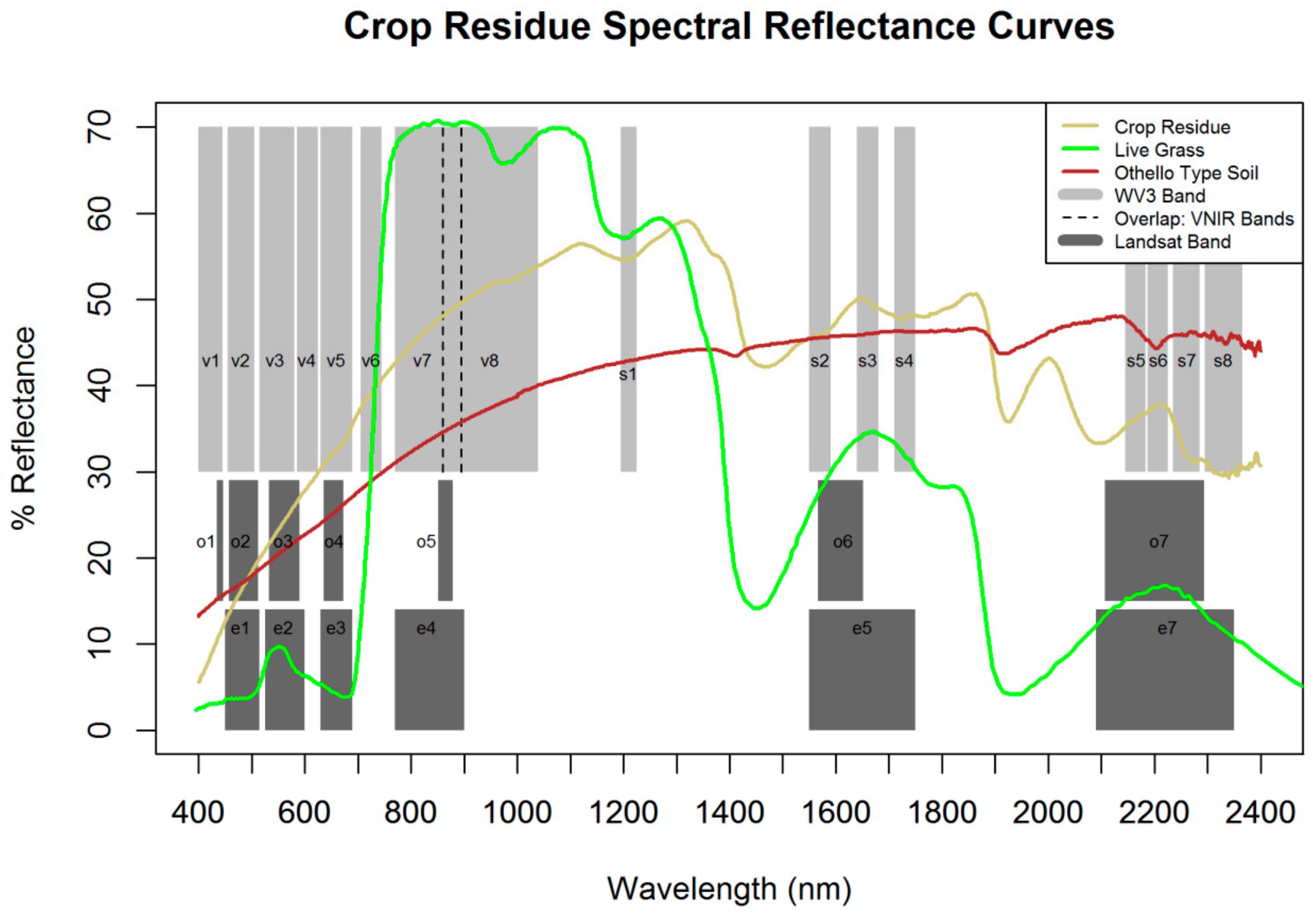
1.4. Remote Sensing of Crop Residue
2. Materials and Methods
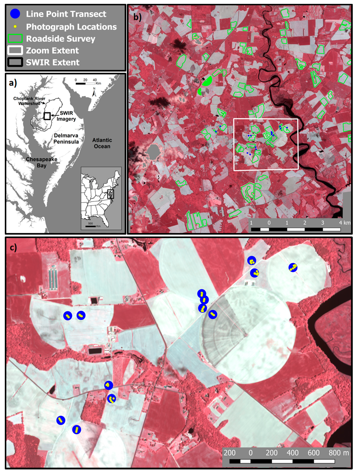
2.1. Site Location
2.2. Satellite Imagery Acquisition
2.3. Calculation of Crop Residue and Vegetation Indices
2.4. Field Sampling
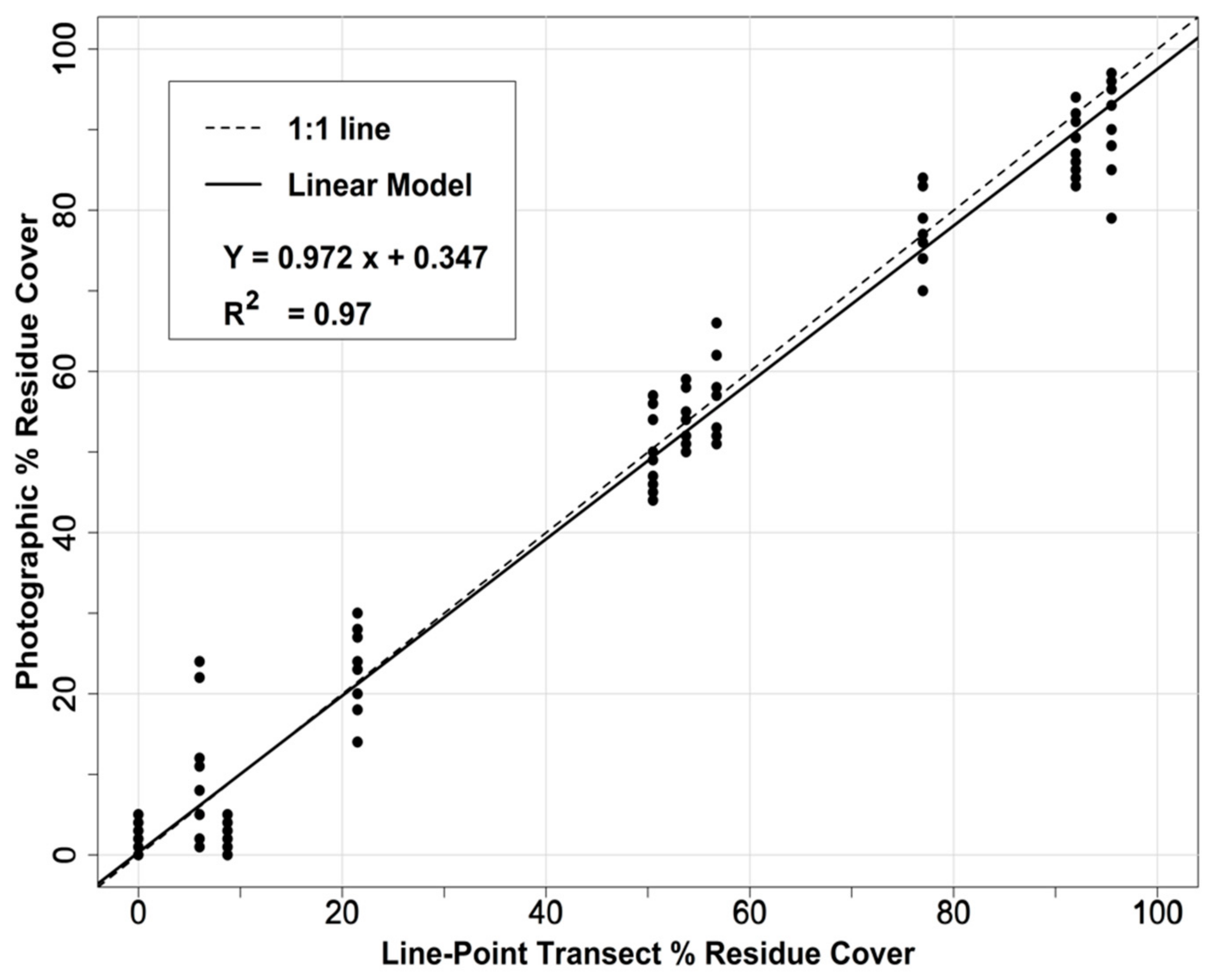
2.4.1. Line-Point Transect
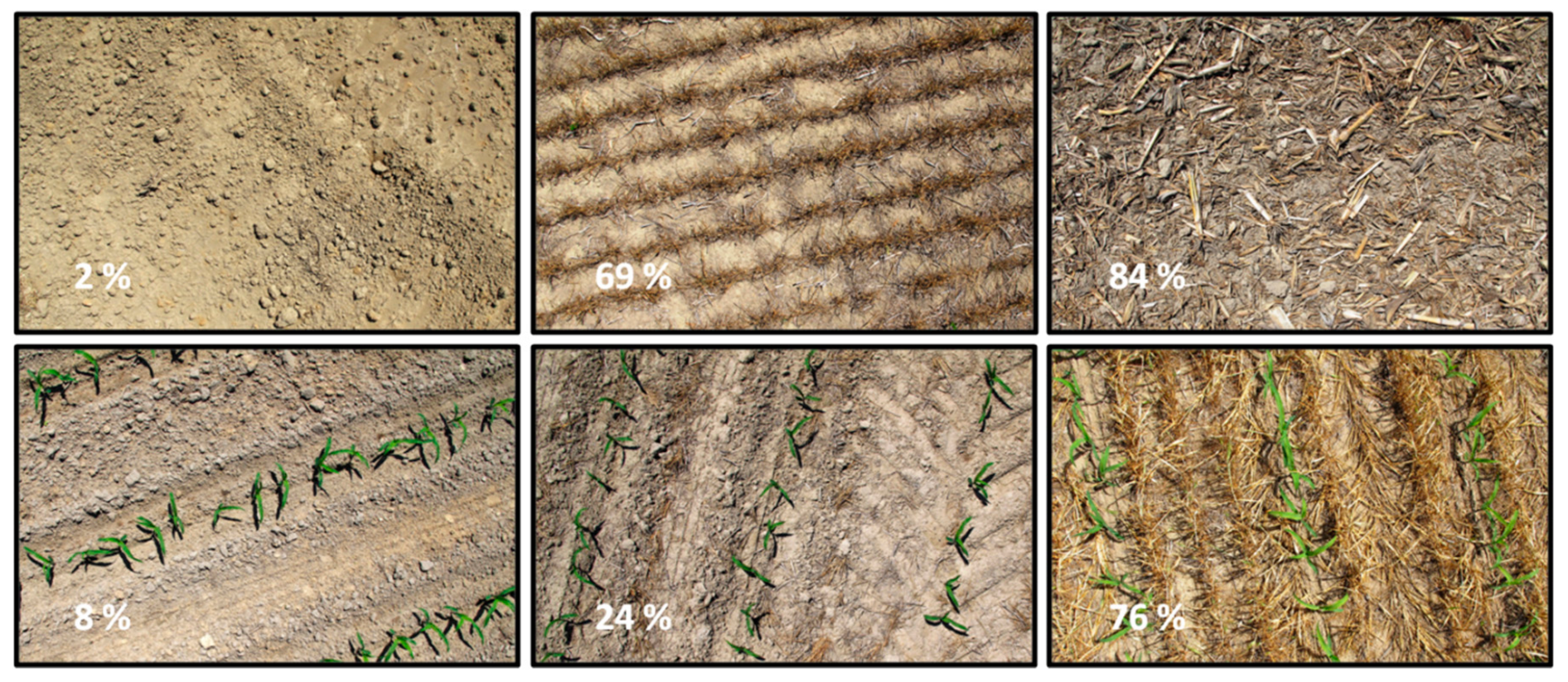
2.4.2. Vertical Digital Photographs
2.5. Roadside Survey
2.6. Calibration and Map Production
3. Results and Discussion
3.1. Results of In-Field Sampling
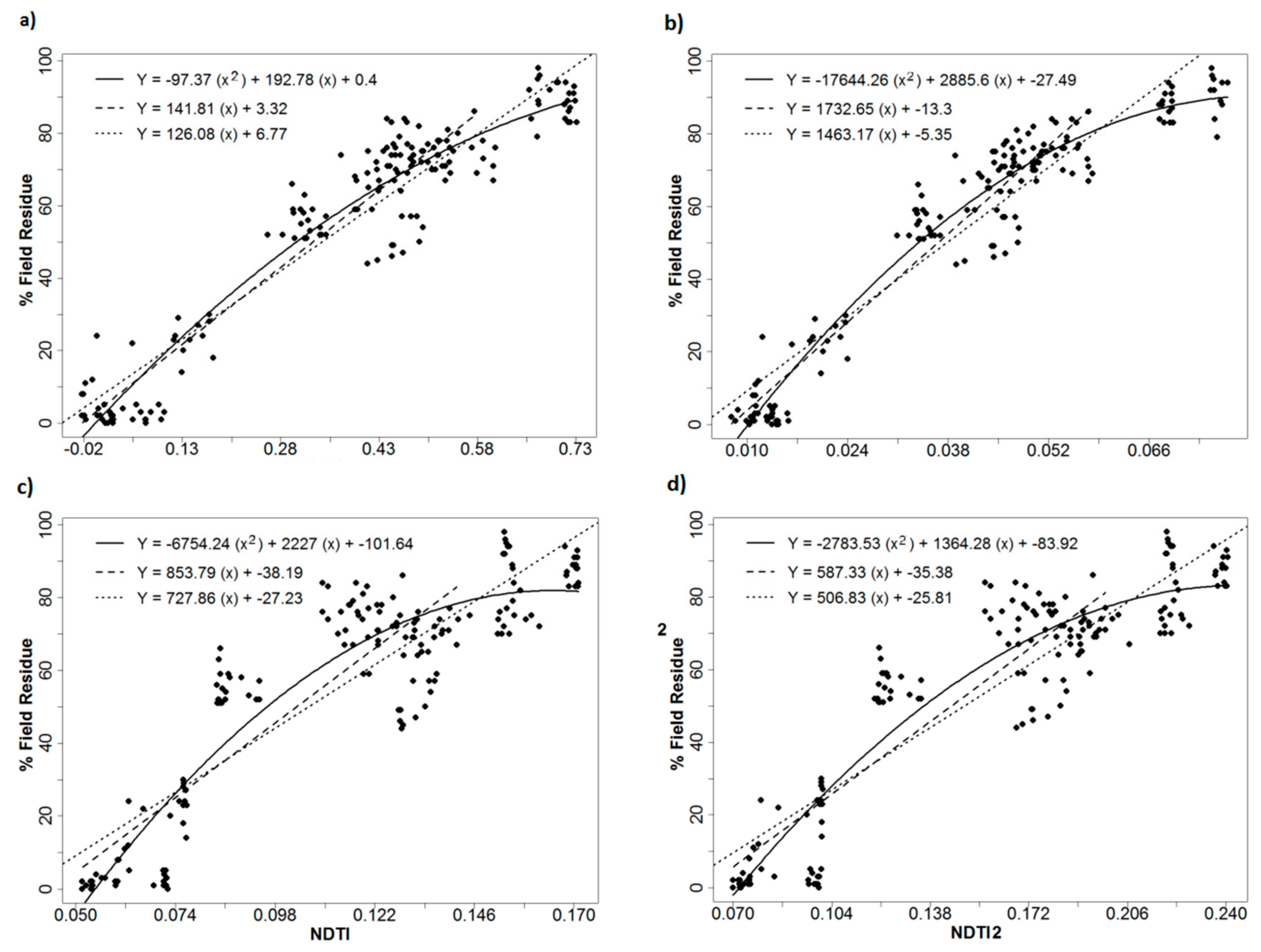
3.2. Index Performance
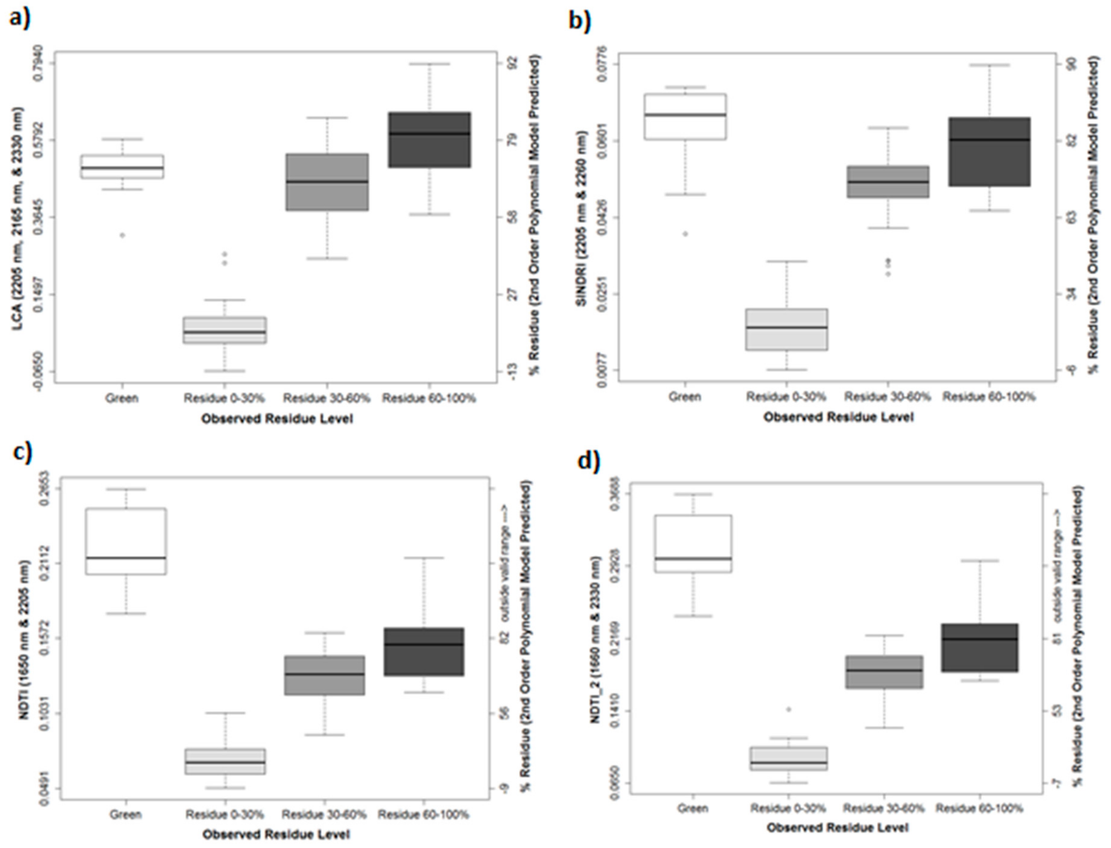
3.3. Roadside Survey and Effect of Vegetation on Residue Indices
3.4. Additional Factors Influencing SWIR Indices
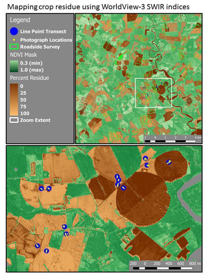
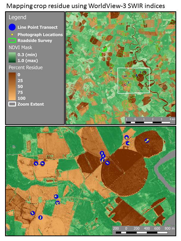
3.5. Mapping Crop Residue Cover in the Landscape
4. Conclusions
Author Contributions
Funding and Disclaimer
Acknowledgments
Conflicts of Interest
Data Availability
Selected Abbreviations
| ANOVA | Analysis of Variance statistical test |
| LCA | Lignin Cellulose Absorption Index |
| ASTER | Advanced Spaceborne Thermal Emission and Reflection Radiometer |
| CAI | Hyperspectral Cellulose Absorption Index |
| CTIC | Conservation Technology Information Center |
| DN | Digital Number |
| LCA | Lignin Cellulose Absorption Index |
| NDTI | Normalized Difference Tillage Index |
| NDVI | Normalized Difference Vegetation Index |
| SINDRI | Shortwave Infrared Normalized Difference Residue Index |
| SWIR | Shortwave infrared wavelengths (1100–2500 nm) |
| TOA | Top of Atmosphere radiance |
| USDA-ARS | U.S. Department of Agriculture, Agricultural Research Service |
| USDA-NASSUSDA-NRCS | U.S. Department of Agriculture, National Agricultural Statistics ServiceU.S. Department of Agriculture, Natural Resources Conservation Service |
| USGS | U.S. Geological Survey |
| VNIR | Visible through near infrared wavelengths (380–1100 nm) |
| WV3 | WorldView-3 satellite |
References
- Delgado, J.A. Crop residue is a key for sustaining maximum food production and for conservation of our biosphere. J. Soil Water Conserv. 2010, 65, 111A–116A. [Google Scholar] [CrossRef]
- Magdoff, F.; Weil, R. Soil Organic Matter Management Strategies. In Soil Organic Matter in Sustainable Agriculture; CRC Press: Boca Raton, FL, USA, 2004. [Google Scholar]
- Palm, C.; Blanco-Canqui, H.; DeClerck, F.; Gatere, L.; Grace, P. Conservation agriculture and ecosystem services: An overview. Agric. Ecosyst. Environ. 2014, 187, 87–105. [Google Scholar] [CrossRef] [Green Version]
- Mulkey, A.S.; Coale, F.J.; Vadas, P.A.; Shenk, G.W.; Bhatt, G.X. Revised Method and Outcomes for Estimating Soil Phosphorus Losses from Agricultural Land in the Chesapeake Bay Watershed Model. J. Environ. Qual. 2017, 46, 1388–1394. [Google Scholar] [CrossRef] [PubMed]
- FAO (Food and Agriculture Organization of the United Nations). Conservation Agriculture. Available online: http://www.fao.org/conservation-agriculture/en/ (accessed on 10 October 2018).
- Hobbs, P.R.; Sayre, K.; Gupta, R. The role of conservation agriculture in sustainable agriculture. Philos. Trans. R. Soc. B Biol. Sci. 2008, 363, 543–555. [Google Scholar] [CrossRef] [PubMed] [Green Version]
- Kemp, W.M.; Boynton, W.R.; Adolf, J.E.; Boesch, D.F.; Boicourt, W.C.; Brush, G.; Cornwell, J.C.; Fisher, T.R.; Glibert, P.M.; Hagy, J.D.; et al. Eutrophication of Chesapeake Bay: Historical trends and ecological interactions. Mar. Ecol. Prog. Ser. 2005, 303, 1–29. [Google Scholar] [CrossRef]
- Hagy, J.D.; Bonton, W.R.; Keefe, C.W.; Wood, K.V. Hypoxia in Chesapeake Bay, 1950–2001: Long-term change in relation to nutrient loading and river flow. Estuaries 2004, 27, 634–658. [Google Scholar] [CrossRef]
- Jordan, T.E.; Correll, D.L.; Weller, D.E. Effects of agriculture on discharges of nutrients from coastal plain watersheds of Chesapeake Bay. J. Am. Water Resour. Assoc. 1997, 33, 631–645. [Google Scholar] [CrossRef]
- Chesapeake Bay Program. Conservation Tillage Practices for Use in Phase 6.0 of the Chesapeake Bay Program Watershed Model; Chesapeake Bay Program: Annapolis, MD, USA, 2016. [Google Scholar]
- Papendick, R.I.; Parr, J.F.; Meyer, R.E. Managing Crop Residues to Optimize Crop/Livestock Production Systems for Dryland Agriculture. In Dryland Agriculture Strategies for Sustainability; Springer: New York, NY, USA, 1990; pp. 253–272. [Google Scholar]
- Godwin, R.J. Agricultural Engineering in Development: Tillage for Crop Production in Areas of Low Rainfall; FAO: Rome, Italy, 1990; Volume 83, p. 129. [Google Scholar]
- Bonham, C.D. Measurements for Terrestrial Vegetation; John Wiley & Sons: New York, NY, USA, 1989; ISBN 0471048801. [Google Scholar]
- Barnes, E.M.; Sudduth, K.A.; Hummel, J.W.; Lesch, S.M.; Corwin, D.L.; Yang, C.; Daughtry, C.S.T.; Bausch, W.C. Remote- and Ground-Based Sensor Techniques to Map Soil Properties. Photogramm. Eng. Remote Sens. 2003, 69, 619–630. [Google Scholar] [CrossRef]
- Bannari, A.; Pacheco, A.; Staenz, K.; McNairn, H.; Omari, K. Estimating and mapping crop residues cover on agricultural lands using hyperspectral and IKONOS data. Remote Sens. Environ. 2006, 104, 447–459. [Google Scholar] [CrossRef]
- Beeson, P.C.; Daughtry, C.S.T.; Hunt, E.R.; Akhmedov, B.; Sadeghi, A.M.; Karlen, D.L.; Tomer, M.D. Multispectral satellite mapping of crop residue cover and tillage intensity in Iowa. J. Soil Water Conserv. 2016, 71, 385–395. [Google Scholar] [CrossRef] [Green Version]
- Corak, S.J.; Kaspar, T.C.; Meek, D.W. Evaluating methods for measuring residue cover. J. Soil Water Conserv. 1993, 48, 70–74. [Google Scholar]
- Gelder, B.K.; Kaleita, A.L.; Cruse, R.M. Estimating mean field residue cover on midwestern soils using satellite imagery. Agron. J. 2009, 101, 635–643. [Google Scholar] [CrossRef]
- Thoma, D.P.; Gupta, S.C.; Bauer, M.E. Evaluation of optical remote sensing models for crop residue cover assessment. J. Soil Water Conserv. 2004, 59, 224–233. [Google Scholar]
- Booth, D.T.; Cox, S.E.; Berryman, R.D. Point sampling digital imagery with “Samplepoint”. Environ. Monit. Assess. 2006, 123, 97–108. [Google Scholar] [CrossRef] [PubMed]
- Morrison, J.E., Jr.; Huang, C.; Lightle, D.T.; Daughtry, C.S.T. Residue Cover Measurement Techniques. J. Soil Water Conserv. 1993, 48, 478–483. [Google Scholar]
- Zheng, B.; Campbell, J.B.; Serbin, G.; Galbraith, J.M. Remote sensing of crop residue and tillage practices: Present capabilities and future prospects. Soil Tillage Res. 2014, 138, 26–34. [Google Scholar] [CrossRef]
- Daughtry, C.S.T. Agroclimatology: Discriminating crop residues from soil by shortwave infrared reflectance. Agron. J. 2001, 93, 125–131. [Google Scholar] [CrossRef]
- Daughtry, C.S.T.; Hunt, E.R.; McMurtrey, J.E. Assessing crop residue cover using shortwave infrared reflectance. Remote Sens. Environ. 2004, 90, 126–134. [Google Scholar] [CrossRef]
- Serbin, G.; Daughtry, C.S.T.; Hunt, E.R.; Reeves, J.B.; Brown, D.J. Effects of soil composition and mineralogy on remote sensing of crop residue cover. Remote Sens. Environ. 2009, 113, 224–238. [Google Scholar] [CrossRef]
- Workman, J.J.; Weyer, L. Practical Guide to Interpretive Near-Infrared Spectroscopy; CRC Press: Boco Raton, FL, USA, 2008; ISBN 1-57444-784-X. [Google Scholar]
- Bégué, A.; Arvor, D.; Bellon, B.; Betbeder, J.; de Abelleyra, D.; Ferraz, R.P.D.; Lebourgeois, V.; Lelong, C.; Simões, M.; Verón, S.R. Remote sensing and cropping practices: A review. Remote Sens. 2018, 10, 99. [Google Scholar] [CrossRef]
- Gausman, H.W.; Leamer, R.W.; Noriega, J.R.; Rodriguez, R.R.; Wiegand, C.L. Field-Measured Spectroradiometric Reflectances of Disked and Non-Disked Soil with and without Wheat Straw. Soil Sci. Soc. Am. J. 1977, 41, 793–796. [Google Scholar] [CrossRef]
- Daughtry, C.S.T.; Doraiswamy, P.C.; Hunt, E.R.; Stern, A.J.; McMurtrey, J.E.; Prueger, J.H. Remote sensing of crop residue cover and soil tillage intensity. Soil Tillage Res. 2006, 91, 101–108. [Google Scholar] [CrossRef]
- Bannari, A.; Staenz, K.; Champagne, C.; Khurshid, K.S. Spatial variability mapping of crop residue using hyperion (EO-1) hyperspectral data. Remote Sens. 2015, 7, 8107–8127. [Google Scholar] [CrossRef]
- Sonmez, N.K.; Slater, B. Measuring intensity of tillage and plant residue cover using remote sensing. Eur. J. Remote Sens. 2016, 49, 121–135. [Google Scholar] [CrossRef]
- Digital Globe. Worldview-3 Fact Sheet. Available online: http://content.satimagingcorp.com.s3.amazonaws.com/media/pdf/WorldView-3-PDF-Download.pdf (accessed on 10 October 2018).
- Biard, F.; Baret, F. Crop residue estimation using multiband reflectance. Remote Sens. Environ. 1997, 59, 530–536. [Google Scholar] [CrossRef]
- Van Deventer, P.; Ward, D.; Gowda, P.H.M.; Lyon, J.G. Using thematic mapper data to identify contrasting soil plains and tillage practices. Photogramm. Eng. Remote Sens. 1997, 63, 87–93. [Google Scholar]
- Sullivan, D.G.; Strickland, T.C.; Masters, M.H. Satellite mapping of conservation tillage adoption in the Little River experimental watershed, Georgia. J. Soil Water Conserv. 2008, 63, 112–119. [Google Scholar] [CrossRef]
- Zheng, B.; Campbell, J.B.; de Beurs, K.M. Remote sensing of crop residue cover using multi-temporal Landsat imagery. Remote Sens. Environ. 2012, 117, 177–183. [Google Scholar] [CrossRef]
- Quemada, M.; Daughtry, C.S.T. Spectral indices to improve crop residue cover estimation under varying moisture conditions. Remote Sens. 2016, 8, 660. [Google Scholar] [CrossRef]
- Satellite Imaging Corporation. WorldView-3 Satellite Sensor. Available online: http://www.satimagingcorp.com/satellite-sensors/worldview-3/ (accessed on 8 August 2018).
- Galloza, M.S.; Crawford, M.M.; Heathman, G.C. Crop residue modeling and mapping using Landsat, ALI, Hyperion, airborne remote sensing data. IEEE J. Sel. Top. Appl. Earth Obs. Remote Sens. 2013, 6, 446–456. [Google Scholar] [CrossRef]
- Serbin, G.; Hunt, E.R.; Daughtry, C.S.T.; McCarty, G.W.; Doraiswamy, P.C. An improved ASTER index for remote sensing of crop residue. Remote Sens. 2009, 1, 971–991. [Google Scholar] [CrossRef]
- Serbin, G.; Daughtry, C.S.T.; Hunt, E.R.; Brown, D.J.; McCarty, G.W. Effect of Soil Spectral Properties on Remote Sensing of Crop Residue Cover. Soil Sci. Soc. Am. J. 2009, 73, 1545–1558. [Google Scholar] [CrossRef]
- De Paul, O.V. Review Article: Remote Sensing, Surface Residue Cover and Tillage Practice. J. Environ. Prot. 2012, 3, 211–217. [Google Scholar] [CrossRef]
- Daughtry, C.S.T.; Hunt, E.R. Mitigating the effects of soil and residue water contents on remotely sensed estimates of crop residue cover. Remote Sens. Environ. 2008, 112, 1647–1657. [Google Scholar] [CrossRef]
- Quemada, M.; Hively, W.D.; Daughtry, C.S.T.; Lamb, B.T.; Shermeyer, J. Improved crop residue cover estimates obtained by coupling spectral indices for residue and moisture. Remote Sens. Environ. 2018, 206, 33–44. [Google Scholar] [CrossRef]
- Daughtry, C.S.T.; Serbin, G.; Reeves, J.B.; Doraiswamy, P.C.; Hunt, E.R. Spectral reflectance of wheat residue during decomposition and remotely sensed estimates of residue cover. Remote Sens. 2010, 2, 416–431. [Google Scholar] [CrossRef]
- R-CoreTeam. R: A Language and Environment for Statistical Computing; R Foundation for Statistical Computing: Vienna, Austria; Available online: http://www.r-project.org/ (accessed on 10 October 2018).
- Serbin, G.; Raymond Hunt, E.; Daughtry, C.S.T.; McCarty, G.W. Assessment of spectral indices for cover estimation of senescent vegetation. Remote Sens. Lett. 2013, 4, 552–560. [Google Scholar] [CrossRef]
- Rouse, J.W.; Haas, R.W.; Schell, J.A.; Deering, D.W.; Harlan, J.C. Monitoring the Vernal Advancement and Retrogradation (Greenwave Effect) of Natural Vegetation; NASA/GSFC Type-III Final Report; National Aeronautics and Space Administration: Greenbelt, MD, USA, 1974; 164p. [Google Scholar]
- U.S. Department of Agriculture. National Cropland Data Layer. Available online: https://nassgeodata.gmu.edu/CropScape/ (accessed on 10 October 2018).
- Hively, W.D.; Lamb, B.T.; Daughtry, C.S.T.; Shermeyer, J.; McCarty, G.M.; Quemada, M. WorldView-3 Satellite Imagery and Crop Residue Field Data Collection. Talbot County, MD, May 2015. U.S. Geological Survey data release. 2018. Available online: https://doi.org/10.5066/F7930SDB (accessed on 10 October 2018).


| Sensor | Band | Name | Range (nm) |
|---|---|---|---|
| VNIR | v1 | Coastal | 400–450 |
| VNIR | v2 | Blue | 448–510 |
| VNIR | v3 | Green | 510–580 |
| VNIR | v4 | Yellow | 585–625 |
| VNIR | v5 | Red | 630–690 |
| VNIR | v6 | Red Edge | 705–745 |
| VNIR | v7 | NIR1 | 770–895 |
| VNIR | v8 | NIR2 | 860–1040 |
| SWIR | s1 | SWIR1 | 1195–1225 |
| SWIR | s2 | SWIR2 | 1550–1590 |
| SWIR | s3 | SWIR3 | 1640–1680 |
| SWIR | s4 | SWIR4 | 1710–1750 |
| SWIR | s5 | SWIR5 | 2145–2185 |
| SWIR | s6 | SWIR6 | 2185–2225 |
| SWIR | s7 | SWIR7 | 2235–2285 |
| SWIR | s8 | SWIR8 | 2295–2365 |
| Index | ||||||||
|---|---|---|---|---|---|---|---|---|
| LCA | SINDRI | SINDRI2 | SINDRI3 | SINDRI4 | SINDRI5 | NDTI | NDTI2 | |
| R2: 2nd order polynomial | 0.92 | 0.94 | 0.92 | 0.93 | 0.87 | 0.90 | 0.84 | 0.86 |
| R2: 1st order linear fit below threshold | 0.90 | 0.90 | 0.88 | 0.89 | 0.82 | 0.87 | 0.76 | 0.80 |
| R2: 1st order full range linear fit | 0.90 | 0.89 | 0.88 | 0.90 | 0.81 | 0.87 | 0.77 | 0.81 |
| RMSE: 2nd order polynomial | 8.40 | 7.15 | 8.17 | 7.81 | 10.61 | 9.27 | 12.00 | 11.10 |
| RMSE: 1st order linear fit below threshold | 9.14 | 8.45 | 9.41 | 8.78 | 12.79 | 10.25 | 14.76 | 13.21 |
| RMSE: 1st order full range linear fit | 9.64 | 9.97 | 10.39 | 9.65 | 13.07 | 10.62 | 14.25 | 12.92 |
| Saturation threshold index value | 0.575 | 0.058 | 0.026 | 0.073 | 0.000 | 0.090 | 0.142 | 0.199 |
| Saturation threshold percent residue | 84.9 | 87.4 | 85.0 | 82.6 | 87.3 | 81.3 | 82.9 | 81.2 |
| Index value 30% residue (2nd order) | 0.188 | 0.025 | 0.023 | 0.036 | -0.019 | 0.048 | 0.080 | 0.111 |
| Index value 60% residue (2nd order) | 0.400 | 0.042 | 0.036 | 0.057 | -0.009 | 0.072 | 0.115 | 0.162 |
| Index | ||||||||||
|---|---|---|---|---|---|---|---|---|---|---|
| Statistic | Cal/Val | Regression Type | LCA | SINDRI | SINDRI2 | SINDRI3 | SINDRI4 | SINDRI5 | NDTI | NDTI2 |
| Goodness of fit (R2) | ||||||||||
| Average | Calibration | 1st order linear fit | 0.902 | 0.895 | 0.886 | 0.900 | 0.818 | 0.877 | 0.781 | 0.818 |
| Min | Calibration | 1st order linear fit | 0.895 | 0.889 | 0.879 | 0.894 | 0.810 | 0.870 | 0.763 | 0.806 |
| Max | Calibration | 1st order linear fit | 0.909 | 0.906 | 0.894 | 0.910 | 0.826 | 0.887 | 0.791 | 0.827 |
| Average | Calibration | 2nd order polynomial | 0.927 | 0.948 | 0.933 | 0.936 | 0.884 | 0.907 | 0.847 | 0.868 |
| Min | Calibration | 2nd order polynomial | 0.921 | 0.945 | 0.928 | 0.932 | 0.877 | 0.903 | 0.841 | 0.863 |
| Max | Calibration | 2nd order polynomial | 0.935 | 0.952 | 0.936 | 0.943 | 0.890 | 0.916 | 0.853 | 0.875 |
| Average | Validation | 1st order linear fit | 0.867 | 0.861 | 0.843 | 0.873 | 0.756 | 0.855 | 0.723 | 0.780 |
| Min | Validation | 1st order linear fit | 0.816 | 0.815 | 0.799 | 0.823 | 0.687 | 0.792 | 0.676 | 0.730 |
| Max | Validation | 1st order linear fit | 0.896 | 0.890 | 0.881 | 0.897 | 0.805 | 0.884 | 0.801 | 0.830 |
| Average | Validation | 2nd order polynomial | 0.893 | 0.914 | 0.887 | 0.910 | 0.818 | 0.886 | 0.788 | 0.827 |
| Min | Validation | 2nd order polynomial | 0.861 | 0.895 | 0.858 | 0.879 | 0.751 | 0.843 | 0.750 | 0.792 |
| Max | Validation | 2nd order polynomial | 0.925 | 0.932 | 0.912 | 0.937 | 0.859 | 0.920 | 0.824 | 0.863 |
| Residual mean squared error (RMSE) | ||||||||||
| Average | Calibration | 1st order linear fit | 9.49 | 9.79 | 10.20 | 9.55 | 12.90 | 10.62 | 14.16 | 12.90 |
| Min | Calibration | 1st order linear fit | 9.17 | 9.49 | 10.05 | 9.24 | 12.70 | 10.22 | 13.68 | 12.46 |
| Max | Calibration | 1st order linear fit | 9.77 | 10.06 | 10.42 | 9.90 | 13.25 | 10.98 | 14.38 | 13.22 |
| Average | Calibration | 2nd order polynomial | 8.18 | 6.87 | 7.85 | 7.64 | 10.28 | 9.22 | 11.82 | 10.99 |
| Min | Calibration | 2nd order polynomial | 7.65 | 6.55 | 7.64 | 7.15 | 9.91 | 8.66 | 11.46 | 10.58 |
| Max | Calibration | 2nd order polynomial | 8.54 | 7.15 | 8.19 | 7.95 | 10.70 | 9.52 | 12.09 | 11.33 |
| Average | Validation | 1st order linear fit | 10.28 | 10.75 | 11.22 | 10.06 | 13.83 | 10.63 | 14.63 | 13.01 |
| Min | Validation | 1st order linear fit | 9.13 | 9.62 | 10.27 | 8.60 | 12.37 | 9.09 | 13.74 | 11.68 |
| Max | Validation | 1st order linear fit | 11.35 | 12.12 | 11.98 | 11.38 | 14.66 | 12.14 | 16.35 | 14.68 |
| Average | Validation | 2nd order polynomial | 9.25 | 8.21 | 9.37 | 8.45 | 11.87 | 9.49 | 12.71 | 11.53 |
| Min | Validation | 2nd order polynomial | 7.90 | 7.20 | 8.13 | 7.27 | 10.30 | 8.32 | 11.77 | 10.27 |
| Max | Validation | 2nd order polynomial | 11.03 | 9.24 | 10.06 | 10.09 | 13.12 | 11.50 | 14.01 | 13.03 |
| Index | ||||||||
|---|---|---|---|---|---|---|---|---|
| LCA | SINDRI | SINDRI2 | SINDRI3 | SINDRI4 | SINDRI5 | NDTI | NDTI2 | |
| 0–30% mean index value | 0.0657 | 0.0178 | −0.0036 | 0.0263 | −0.0241 | 0.035 | 0.0693 | 0.0922 |
| 0–30% mean, calculated % residue | 12.6 | 18.2 | 15.3 | 15.6 | 10.8 | 14.7 | 20.3 | 18.2 |
| p-value 0–30% vs. 30–60% | <0.0001 | <0.0001 | <0.0001 | <0.0001 | <0.0001 | <0.0001 | <0.0001 | <0.0001 |
| 30–60% mean index value | 0.4555 | 0.0487 | 0.0202 | 0.0636 | −0.007 | 0.0788 | 0.1292 | 0.1801 |
| 30–60% mean, calculated % residue | 68.0 | 71.2 | 70.2 | 69.0 | 69.3 | 67.3 | 73.4 | 71.5 |
| p-value 30–60% vs. 60–100% | <0.0001 | 0.0017 | <0.0001 | 0.0006 | <0.0001 | 0.0005 | 0.0058 | 0.0027 |
| 60–100% mean index value | 0.5764 | 0.0593 | 0.0284 | 0.0768 | −0.0006 | 0.095 | 0.1528 | 0.2163 |
| 60–100% mean, calculated % residue | 79.2 | 81.5 | 81.1 | 80.2 | 79.9 | 78.9 | 81.0 | 80.9 |
| Green mean index value | 0.4957 | 0.0632 | 0.0327 | 0.0911 | 0.0041 | 0.1206 | 0.2207 | 0.309 |
| Green mean, calculated % residue | 72.0 | 84.4 | 85.0 | 87.7 | 83.7 | 88.7 | * | * |
| p-value Green-0–30% | <0.0001 | <0.0001 | <0.0001 | <0.0001 | <0.0001 | <0.0001 | <0.0001 | <0.0001 |
| p-value Green-30–60% | 0.5935 | <0.0001 | <0.0001 | <0.0001 | <0.0001 | <0.0001 | <0.0001 | <0.0001 |
| p-value Green-60–100% | 0.0784 | 0.6095 | 0.2364 | 0.0017 | 0.0277 | <0.0001 | <0.0001 | <0.0001 |
| * outside valid range | ||||||||
| a) SINDRI | b) LCA | ||||||||
| Roadside | Spectral Index Prediction | Roadside | Spectral Index Prediction | ||||||
| survey | 0–30 | 30–60 | 60–100 | % | survey | 0–30 | 30–60 | 60–100 | % |
| 0–30 | 14 | 2 | 1 | 0.82 | 0–30 | 14 | 0 | 3 | 0.82 |
| 30–60 | 0 | 5 | 24 | 0.17 | 30–60 | 1 | 9 | 19 | 0.31 |
| 60–100 | 0 | 0 | 22 | 1.00 | 60–100 | 0 | 1 | 21 | 0.95 |
| % | 1.00 | 0.71 | 0.47 | 0.60 | 0.93 | 0.90 | 0.49 | 0.65 | |
| c) NDTI | d) NDTI2 | ||||||||
| Roadside | Spectral Index Prediction | Roadside | Spectral Index Prediction | ||||||
| survey | 0–30 | 30–60 | 60–100 | % | survey | 0–30 | 30–60 | 60–100 | % |
| 0–30 | 14 | 2 | 1 | 0.82 | 0–30 | 14 | 2 | 1 | 0.82 |
| 30–60 | 0 | 4 | 25 | 0.14 | 30–60 | 0 | 5 | 24 | 0.17 |
| 60–100 | 0 | 0 | 22 | 1.00 | 60–100 | 0 | 0 | 22 | 1.00 |
| % | 1.00 | 0.67 | 0.46 | 0.59 | % | 1.00 | 0.71 | 0.47 | 0.60 |
© 2018 by the authors. Licensee MDPI, Basel, Switzerland. This article is an open access article distributed under the terms and conditions of the Creative Commons Attribution (CC BY) license (http://creativecommons.org/licenses/by/4.0/).
Share and Cite
Hively, W.D.; Lamb, B.T.; Daughtry, C.S.T.; Shermeyer, J.; McCarty, G.W.; Quemada, M. Mapping Crop Residue and Tillage Intensity Using WorldView-3 Satellite Shortwave Infrared Residue Indices. Remote Sens. 2018, 10, 1657. https://doi.org/10.3390/rs10101657
Hively WD, Lamb BT, Daughtry CST, Shermeyer J, McCarty GW, Quemada M. Mapping Crop Residue and Tillage Intensity Using WorldView-3 Satellite Shortwave Infrared Residue Indices. Remote Sensing. 2018; 10(10):1657. https://doi.org/10.3390/rs10101657
Chicago/Turabian StyleHively, W. Dean, Brian T. Lamb, Craig S. T. Daughtry, Jacob Shermeyer, Gregory W. McCarty, and Miguel Quemada. 2018. "Mapping Crop Residue and Tillage Intensity Using WorldView-3 Satellite Shortwave Infrared Residue Indices" Remote Sensing 10, no. 10: 1657. https://doi.org/10.3390/rs10101657
APA StyleHively, W. D., Lamb, B. T., Daughtry, C. S. T., Shermeyer, J., McCarty, G. W., & Quemada, M. (2018). Mapping Crop Residue and Tillage Intensity Using WorldView-3 Satellite Shortwave Infrared Residue Indices. Remote Sensing, 10(10), 1657. https://doi.org/10.3390/rs10101657