Potential of Sentinel-2A Data to Model Surface and Canopy Fuel Characteristics in Relation to Crown Fire Hazard

Abstract

Background: Crown fires are often intense and fast spreading and hence can have serious impacts on soil, vegetation, and wildlife habitats. Fire managers try to prevent the initiation and spread of crown fires in forested landscapes through fuel management. The minimum fuel conditions necessary to initiate and propagate crown fires are known to be strongly influenced by four stand structural variables: surface fuel load (SFL), fuel strata gap (FSG), canopy base height (CBH), and canopy bulk density (CBD). However, there is often a lack of quantitative data about these variables, especially at the landscape scale. Methods: In this study, data from 123 sample plots established in pure, even-aged, Pinus radiata and Pinus pinaster stands in northwest Spain were analyzed. In each plot, an intensive field inventory was used to characterize surface and canopy fuels load and structure, and to estimate SFL, FSG, CBH, and CBD. Equations relating these variables to Sentinel-2A (S-2A) bands and vegetation indices were obtained using two non-parametric techniques: Random Forest (RF) and Multivariate Adaptive Regression Splines (MARS). Results: According to the goodness-of-fit statistics, RF models provided the most accurate estimates, explaining more than 12%, 37%, 47%, and 31% of the observed variability in SFL, FSG, CBH, and CBD, respectively. To evaluate the performance of the four equations considered, the observed and estimated values of the four fuel variables were used separately to predict the potential type of wildfire (surface fire, passive crown fire, or active crown fire) for each plot, considering three different burning conditions (low, moderate, and extreme). The results of the confusion matrix indicated that 79.8% of the surface fires and 93.1% of the active crown fires were correctly classified; meanwhile, the highest rate of misclassification was observed for passive crown fire, with 75.6% of the samples correctly classified. Conclusions: The results highlight that the combination of medium resolution imagery and machine learning techniques may add valuable information about surface and canopy fuel variables at large scales, whereby crown fire potential and the potential type of wildfire can be classified.

1. Introduction

Crown fires are usually more difficult to control than surface fires, due to their higher rate of spread and their higher intensity and spotting activity, demanding massive mobilization of fire-fighting forces. Moreover, their effects on soil, vegetation, and wildlife habitats are usually more severe and lasting than surface fires. Fire managers try to prevent the initiation and spread of crown fires in forested landscapes through fuel management. The allocation of such management activities can be enhanced by fire behavior simulation systems, which require certain fuel variables to be mapped. Spatially-explicit estimates of forest fuels can also serve as valuable information to predict and mitigate the effects of forthcoming wildfires.

Fuel complex structural characteristics that are commonly considered to determine crown fire initiation and spread include surface fuel load, fuel strata gap, canopy base height, and canopy bulk density [1,2]. Surface fuel load (SFL) is the amount of fuel that is potentially available for combustion in the surface fuel complex. It directly affects the surface fireline intensity, and therefore the likelihood of occurrence of vertical fire spread into the canopy. Fuel strata gap (FSG) is defined as the distance from the top of the surface fuelbed to the lower limit of the aerial fuel stratum that can sustain vertical fire propagation [3,4]. Canopy base height (CBH) is usually defined as the lowest height above the ground at which there is sufficient canopy fuel to propagate fire vertically through the canopy [5]. Therefore, both FSG and CBH are a measure of the proximity of canopy fuels to surface fuels [6], and they strongly influence the likelihood of crown fire initiation. Canopy bulk density (CBD) describes the amount of available fuel within a unit volume of the canopy [1]. It is a key variable for discriminating the type of crown fire spread regime [1], and thus for evaluating the fire hazard and how fuel treatments affect crown fire potential.

Remote sensing technologies, including airborne light detection and ranging (LiDAR), and optical satellite imagery, have been used to estimate these surface and canopy fuels variables. LiDAR actively senses the three-dimensional structure of underlying terrain and vegetation, and therefore it has been successfully used to characterize both canopy and surface fuels (e.g., [7,8,9]). However, the temporal and spatial coverage with airborne sensors is limited by the cost of acquisition, which hampers the analysis of fuel dynamics, or leads the analysis focusing on small geographical extents. Optical satellite data provide a cost-effective alternative source for estimating fuel information, since they can offer comprehensive spatial coverage and adequate temporal resolution to update fuel maps.

The main limitations of optical sensors in evaluating forest fuels come from their difficulty to characterize those forest attributes with a strong vertical component [10], besides their problems with penetrating the forest canopy, and hence estimating surface fuels beneath the crowns [11].

In spite of these shortcomings, previous research using a variety of spectral sensors has demonstrated that medium resolution optical data can be used for an accurate estimation of forest fuel variables. Keane et al. [12] estimated CBD and CBH from Landsat TM imagery in the Gila National Forest (New Mexico); the same sensor was subsequently used within the LANDFIRE project for all major vegetation systems in the US [13]. Pierce et al. [14] and Palaiologou et al. [15] integrated Landsat TM data and ancillary information (topographic and climatic variables) for modeling and mapping CBH and CBD variables in mixed conifer forests in California and coastal forests in Greece, respectively, whereas Falkowski et al. [16] used ASTER imagery to estimate CBD in an experimental conifer forest in Ohio.

Concerning surface fuel loads, most studies have focused on forest fuel classification (e.g., [12,15,16]). In most cases, vegetation mapping is performed first, and then each vegetation class is assigned to a fuel model using a look-up table (e.g., [12]). Relatively few studies have been conducted to estimate surface fuel load directly [17,18,19]. Reich et al. [17] developed a linear equation for estimating SFL using Landsat TM reflectance data, and biophysical variables as predictors for the Black Hills National Forest, South Dakota. Brandis and Jacobson [18] indirectly estimated SFL from stand characteristics extracted from Landsat TM data in New South Wales (Australia). Jin and Chen [19] tested both spectral reflectance-based and stand characteristics-based models for estimating fuel loads in the Daxinganling region (northeast China) using Landsat TM and QuickBird imageries.

The new S-2A mission offers an unprecedented combination of spectral and spatial resolution that is expected to provide significant new opportunities in forest fuel modeling and mapping. The incorporation of three narrow bands in the red-edge of the spectrum characterized by a high correlation with vegetation biophysical properties such as chlorophyll content and leaf area index (e.g., [20]), is likely to improve forest fuel estimates. Additionally, the S-2A spatial resolution (10–20 m for the more used bands in vegetation mapping) increased the detail level, compared to the widely used Landsat data (30 m resolution), which is expected to contribute to improving the correlation between forest fuel properties and the remotely sensed data.

For these reasons the use of the S-2A freely–accessible remote sensing information with higher spatial resolution than other approaches used so far (e.g., Landsat), led us to explore its suitability for the operational classification of forest stands in terms of its propensity to different type of crown fires

To the very best of our knowledge S-2A data have been used in studies on tree species classification [21,22], estimation of canopy cover and leaf area index [23], growing stock volume [24,25], and above-ground biomass [26] but there is no experience on its suitability for forest fuel estimation or linking that estimation with potential wildfire behavior. Therefore, the aims of the present study were: (i) to evaluate the potential of S-2A data to estimate surface and canopy fuels variables related to crown fire hazards in pine species; and (ii) to assess the performance of these estimates to classify the expected type wildfires (surface, passive crown fire, or active crown fire) under certain burning conditions.

Accordingly, our main interest is to reach a trade-off between acceptable accuracy in categorizing possible crown fire types, and the use of a free-accessible remote-sensed spectral information to be operationally used by forest managers. Therefore, this study could provide new data on this topic of critical value for landscape fuel management optimization.

2. Materials and Methods

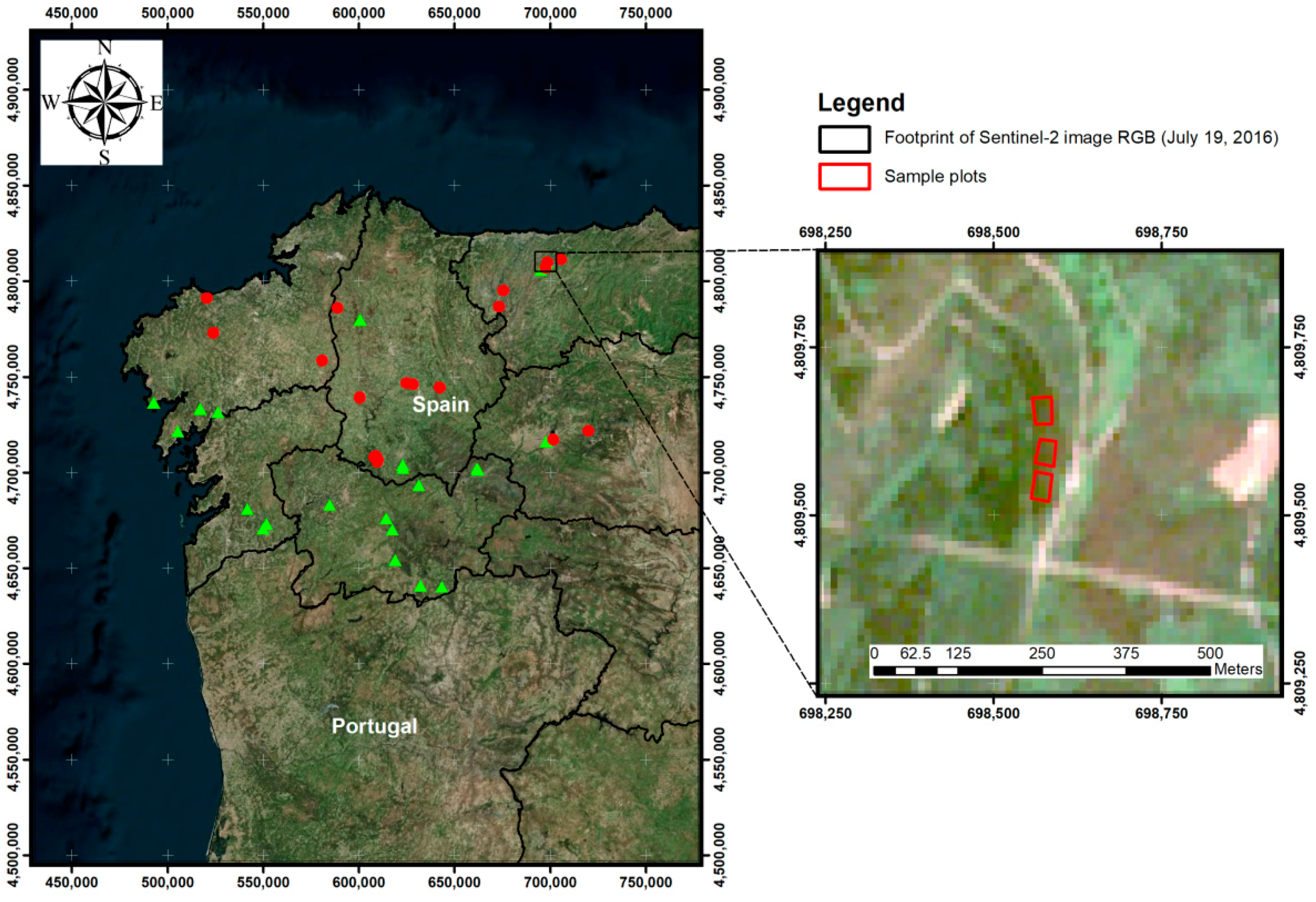
2.1. Plot Network

The study area was located in the northwest of Spain, including the region of Galicia, the western area of the region of Asturias and the western area of the province of León (Figure 1). The dataset corresponds to 41 thinning trial locations installed in pure, even-aged stands of Pinus pinaster (22 locations) and Pinus radiata (19 locations). The thinning trials were established to assess the influence of common fuel and stand descriptors in crown fire potential, and the inventory design was deliberately aimed to represent young and highly stocked stands in the region, because these types of stands are usually particularly fire prone.

At each location, three rectangular plots (1000 m² in size, 40 × 25 m) were established, and a different treatment was applied to each plot: control (unthinned, C), moderate thinning (20% of the basal area removed, MT), and heavy thinning (40% of the basal area removed, HT). The plots were thinned from below immediately after plot establishment in 2010.

The sample plots were georeferenced with a differential GPS to accurately determine the Universal Transverse Mercator (UTM) coordinates of the four corners of each plot. The 123 plots established were re-measured at different age intervals, although in this study, only the measurement carried on the summer of 2016 was used.

2.2. Tree Variables

Diameter at breast height (d) of all the trees was calculated as the average of two perpendicular measurements to the nearest 0.1 cm with a graduated caliper. Total tree height (h) and height to the base of live crown (h_blc, defined as the lower insertion point of live branches in a tree) were measured to the nearest 0.1 m with a digital hypsometer in a randomized sample of 30 trees, and in an additional sample to include all the dominant trees (the proportion of the 100 largest diameter trees per hectare). Generalized h–d models [27] and crown profile models [28,29] developed for these species in the study area were used to estimate h and h_blc for the remaining trees.

The number of stems per hectare (N), stand basal area (G), average stand height ($\overline{h}$), stand dominant height (H₀, defined as the mean height of the 100 thickest trees per hectare) and mean height to the base of live crown ($\overline{h_{blc}}$) were calculated from tree variables.

2.3. Surface Fuel Variables

The surface fuel loads (i.e., loads of shrub and herbaceous fuels, downed woody material, and litter and duff layers) were estimated on control and heavily thinned plots (a total of 82 plots). Due to the complexity of the approach used to estimate the surface fuel loads, the moderately thinned plots were not considered.

For each sample plot, two transects of 32 m each were established from the middle of one of the 40 m sides of the plot to the vertices of the opposite side. The linear coverage of the shrubs and herbaceous fuels, differentiating by species, was recorded along each transect. The depth of the litter and duff layers and the height of the shrub and herbaceous fuels were measured by species every 4 m along each transect. The mean height of the shrub and herbaceous fuels (${\overline{h}}_{shrubs}$) and the mean depth of the litter and duff layers ($\overline{d_{LD}}$) were estimated from these measurements.

The shrub, herbaceous, upper duff, and litter layer fuel loads were calculated using the equations proposed by Arellano-Pérez [30] for these types of fuels in pine stands in Galicia. These equations use ${\overline{h}}_{shrubs}$ and $\overline{d_{LD}}$ as input variables.

The downed woody debris (DWD) load was estimated using the planar transect method [31,32,33]. This method is an adaptable technique based on probability–proportional-to-size concepts that have been used extensively in many inventories and monitoring programs because it is relatively fast and simple to use [34,35,36], and at the same time accurate [37,38,39]. The DWD were divided into four commonly accepted size classes [40] that correspond to timelag fuel classes used in fire behavior modeling (see, for example, [41]]: Fine woody debris (FWD) One hour fuels (particles with diameters <0.6 cm in diameter and where 1 h refers to the number of hours that it takes debris of this size to dry enough to reach equilibrium moisture content); FWD 10 h fuels (particles between 0.6 and 2.5 cm in diameter); FWD 100 h fuels (particles 2.5 to 7.6 cm in diameter), and coarse woody debris (CWD) 1000 h fuels (fuel components >7.6 cm in diameter, including all logs). In this study, different segments along each transect were used per size classes: 1 h and 10 h fuels were sampled along 2 m segments, whereas 100 h and 1000 h fuels were sampled along 5 m and 20 m segments, respectively. Subsequently, downed woody material loading was calculated from relationships developed by Brown [32] that use the number of pieces intersected, transect length, and wood-specific gravity.

Surface fuel load (SFL) was finally calculated as the sum of the estimated load for each surface fuel layer (shrubs and herbaceous, downed woody material, and litter and duff layers).

2.4. Canopy Fuel Variables

Three structural canopy fuel variables, at plot scale were estimated from tree and surface fuel measurements: canopy bulk density (CBD), canopy base height (CBH), and fuel strata gap (FSG). We used the ‘load over depth method’ to define these variables, because it is compatible with the canopy fuel stratum characteristics that were used in the crown fire initiation and propagation model developed by Van Wagner [1], which has been implemented in most fire behavior simulation systems (i.e., BehavePlus [42], Farsite [43], FlamMap [44], or CFIS [45]).

According to this method, CBH is calculated as the vertical distance between the ground surface and the mean crown base height, and therefore equals $\overline{h_{blc}}$. FSG was calculated as the difference between CBH and the mean height of surface fuels (${\overline{h}}_{shrubs}$), and CBD was calculated by dividing the available canopy fuel load by the canopy length. Needles and fine twigs (up to 5 mm at the thick end) were considered as available fuel (i.e., the fuel that is assumed to be consumed within the flaming front of a crown fire), and the canopy length was estimated as the difference between $\overline{h}$ and CBH. The compatible systems of tree biomass equations developed for maritime pine and radiata pine in Galicia [27] were used to estimate the available canopy fuel.

The mean, maximum, and minimum values and standard deviations for the main tree, stand and canopy, and surface fuel variables are shown in

Table 1. Statistics of the main tree, stand, surface, and canopy fuels variables. Std. dev is the standard deviation; d = tree diameter, h = tree height, h_blc = tree height to the base of the life crown; t = stand age; N = stem density; G = stand basal area; H = dominant height (defined as the mean height of the 100 thickest trees per ha); SFL = surface fuel load (shrubs and herbaceous, downed dead woody surface debris, and litter and duff layers); FSG = fuel strata gap; CBH = canopy base height; CBD = canopy bulk density. * The sample size to calculate FSG and SFL was 82 plots, corresponding to the control (C) and heavily thinned (HT) plots.

Species	Statistic	Tree Variables (n = 10,831)			Stand Variables (n = 123)				Surface and Canopy Fuels Variables (n = 123 *)
		d (cm)	h (m)	hblc (m)	t (years)	N (stems ha−1)	G (m2 ha−1)	H (m)	SFL (Mg ha−1)	FSG (m)	CBH (m)	CBD (kg m−3)
P. pinaster	Mean	21.12	14.96	8.63	23.67	1028.22	39.08	16.08	44.99	8.35	8.66	0.1655
	Std. dev.	6.50	2.96	2.48	4.18	480.64	9.34	2.69	10.22	2.32	2.31	0.0503
	Min.	3.90	5.60	2.3	18	407	20.04	10.98	30.24	4.18	4.53	0.0846
	Max.	48.50	23.7	15.9	38	3095	66.08	21.35	78.49	12.65	13.03	0.3369
P. radiata	Mean	21.92	20.13	10.34	22.43	838.47	34.57	22.67	49.42	9.67	10.15	0.1140
	Std. dev.	6.78	3.88	3.18	2.06	427.53	9.88	2.78	21.28	2.78	2.53	0.0462
	Min.	2.75	5.80	1.10	18	316	15.59	16.15	24.47	4.70	5.51	0.0372
	Max.	47.55	30.10	20.70	28	2899	66.63	27.23	116.03	14.88	15.83	0.2840

.

2.5. Sentinel-2A Data Set

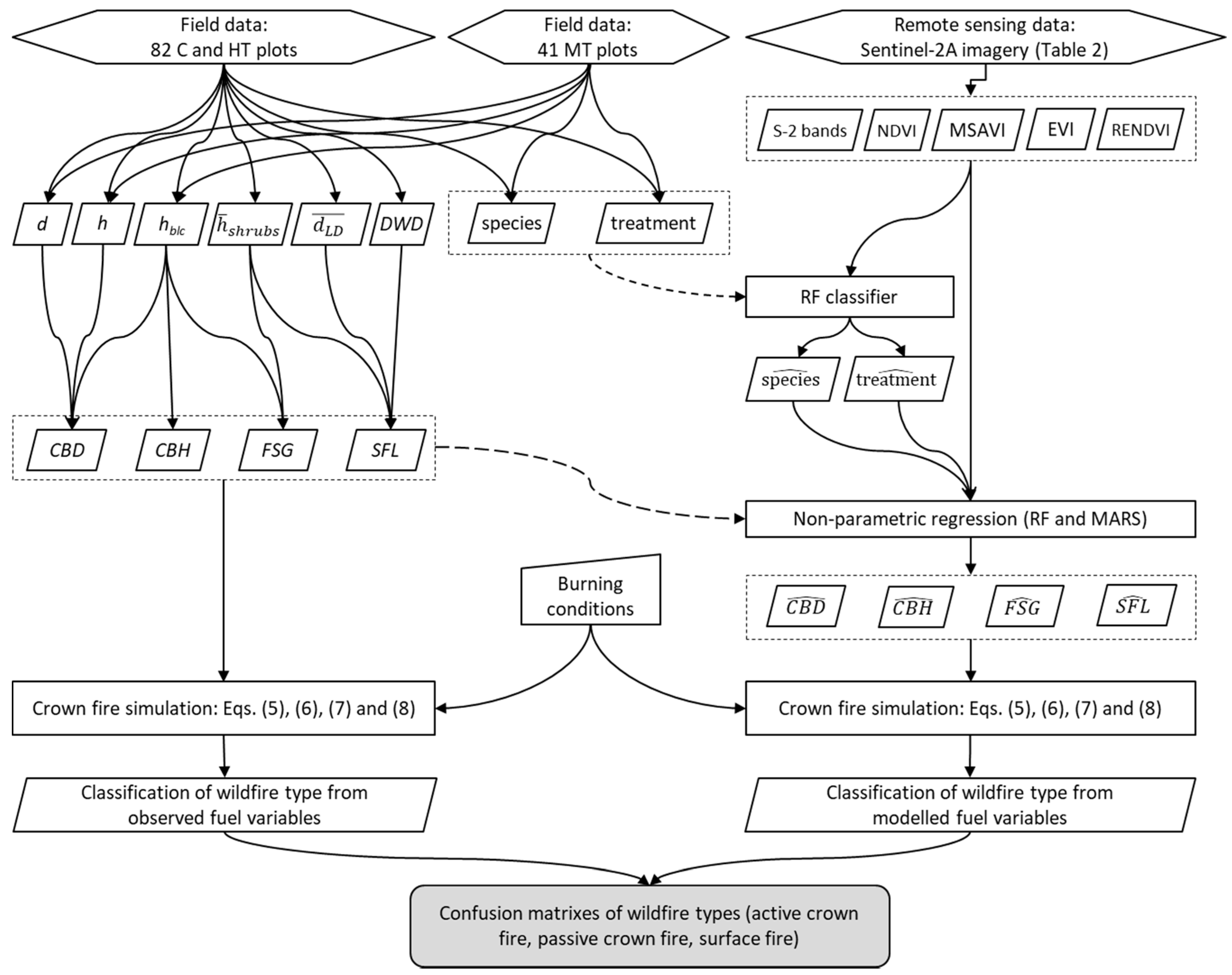
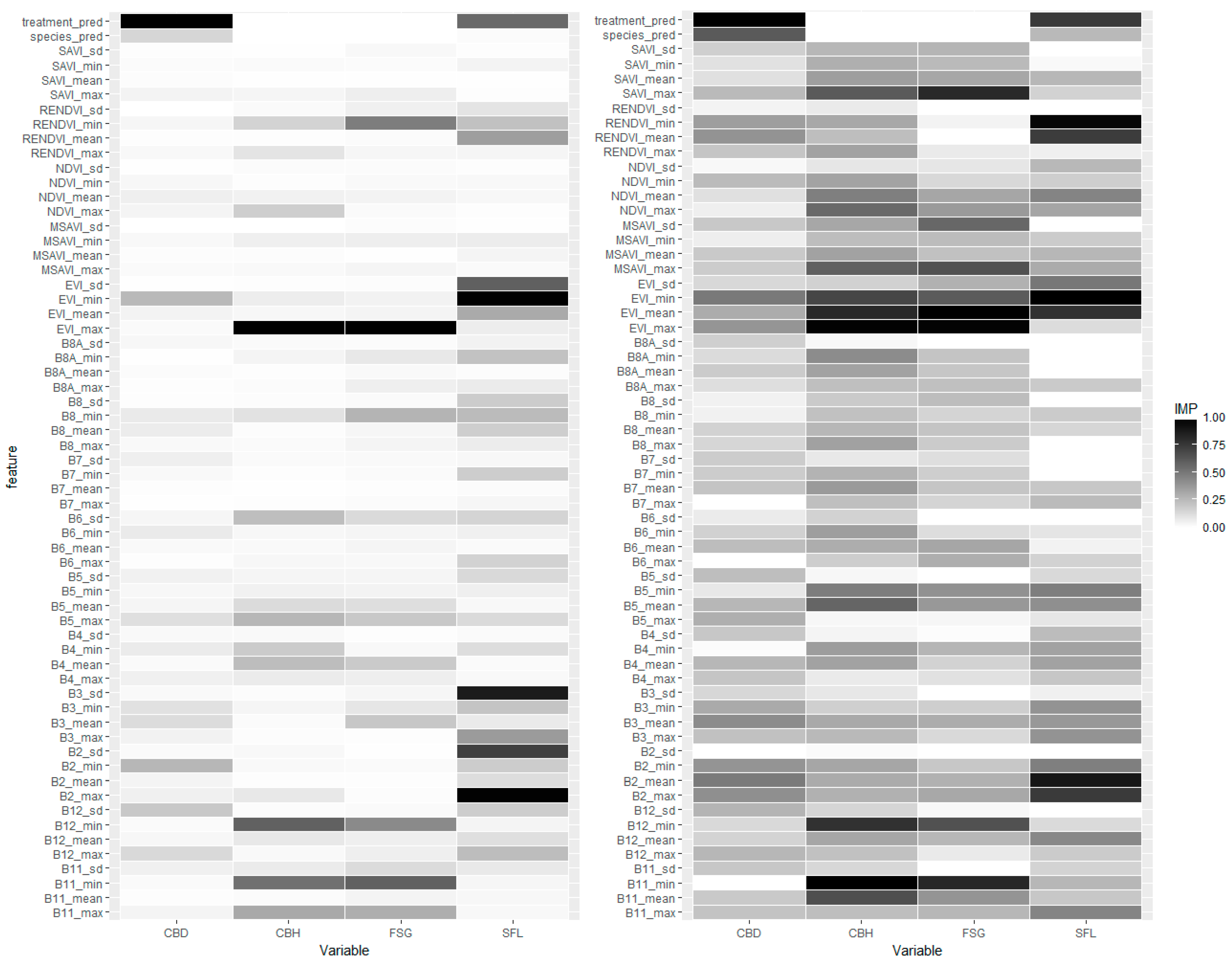
Cloud-free S-2A multispectral instrument (MSI) level 1-C (L1C) imagery acquired on 19 July and 1 August 2016 (

Table 2. Acquisition dates, solar elevation and azimuth angles of S-2A scenes.

Scene	Acquisition Date	Solar Elevation (°)	Solar Azimuth (°)
S-2A_tile_20160801_29TMH	1 August 2016	61.92	148.41
S-2A_tile_20160719_29TNG	19 July 2016	63.25	144.23
S-2A_tile_20160801_29TNH	1 August 2016	61.92	148.41
S-2A_tile_20160719_29TPG	19 July 2016	63.25	144.23
S-2A_tile_20160719_29TPH	19 July 2016	63.25	144.23
S-2A_tile_20160719_29TPJ	19 July 2016	63.25	144.23
S-2A_tile_20160719_29TQH	19 July 2016	63.25	144.23

), matching the field inventory of the sample plots, were downloaded from the U.S. Geological Survey (USGS) Global Visualization Viewer.

The 12-bit S-2A MSI image had 13 spectral bands in the visible (VIS), near-infrared (NIR), and shortwave infrared (SWIR) wavelength regions, with spatial resolutions from 10 to 60 m. For this study, the three “atmospheric” bands (B1, B9, and B10) were discarded (

Table 3. Spatial and spectral resolutions of S-2A/MSI. NIR = near-infrared wavelength region; SWIR = shortwave infrared wavelength region.

Sentinel-2A/MSI (µm)	Band	Resolution (m)
Band 2 (0.46–0.52)	Blue	10
Band 3 (0.54–0.58)	Green	10
Band 4 (0.65–0.68)	Red	10
Band 5 (0.7–0.71)	Red-edge-1	20
Band 6 (0.73–0.75)	Red-edge-2	20
Band 7 (0.76–0.78)	Red-edge-3	20
Band 8 (0.78–0.90)	NIR	10
Band 8A (0.85–0.87)	Narrow NIR	20
Band 11 (1.56–1.65)	SWIR-1	20
Band 12 (2.10–2.28)	SWIR-2	20

).

Since atmospherically-corrected images are essential to assess spectral indices with spatial reliability and product comparisons, L1C data were processed to level-2A (L2A, bottom-of-atmosphere reflectance) by taking into account the effects of aerosols and water vapor on reflectances. These corrections were performed using the ESA’s (European Space Agency, Paris, France) Sen2Cor 2.4 tool [46] for the S-2A images. The data preparation involved the resampling (nearest neighbor) of the S-2A bands acquired at 20 m, to obtain a layer stack of 10 spectral bands at 10 m using the ESA’s S-2 toolbox from the ESA Sentinel Application Platform (SNAP, Paris, France), and then converted to the Environment for Visualizing Images (ENVI) format. Then, the rectified images were used to calculate five vegetation indices (VIs): NDVI, SAVI, MSAVI, EVI, and RENDVI. The normalized difference vegetation index (NDVI) [47] is currently the most widely used VI as a feature for modeling many target variables. The soil-adjusted vegetation index (SAVI) [48] is a refinement of the NDVI, aimed at accounting for uncertainties due to variations in background condition. SAVI incorporated the correction factor L into the NDVI formula. L accounts for soil variation by varying the factor between 1, for low vegetation, and 0, for dense vegetation. In this study, a value of 0.5 was assumed. Qi et al. [49] presented a modified version of the SAVI (MSAVI) which utilized a self-adjusting L factor. The enhanced vegetation index (EVI) was developed by Huete et al. [50] to account for aerosol variation, and also as a vegetation index that was less prone to saturation on dense green vegetation canopy. Finally, the red-edge NDVI (RENDVI) is based on NDVI, but it uses the red-edge spectral band B6 instead of the red spectral band B4 [51]. The formulations and the bands used to estimate the VIs are shown in

Table 4. Formulation of the vegetation indices (VIs) calculated from S-2A image data. NDVI: Normalized difference vegetation index, SAVI: Soil adjusted vegetation index, MSAVI: modified version of the SAVI, EVI: Enhanced vegetation index, B4, B6, B8: 12-bit S-2A bands.

Vegetation Index	Formulation	S-2A Bands Used
NDVI [47]	$\frac{\left(NIR-Red\right)}{\left(NIR+Red\right)}$	$\frac{\left(B8-B4\right)}{\left(B8+B4\right)}$
SAVI [48]	$\frac{\left(1+L\right)\left(NIR-Red\right)}{\left(NIR+Red+L\right)}$	$\frac{\left(1.5\right)\left(B8-B4\right)}{\left(B8+B4+0.5\right)}$
MSAVI [49]	$\begin{array}{c}\frac{\left(1+L\right)\left(NIR-Red\right)}{\left(NIR+Red+L\right)}\\ L=1-\frac{\left(NIR-Red\right)\left(NIR-0.5Red\right)}{\left(NIR+Red\right)}\end{array}$	$\frac{\left(2-\frac{\left(B8-B4\right)\left(B8-0.5B4\right)}{\left(B8+B4\right)}\right)\left(B8-B4\right)}{\left(B8+B4+1-\frac{\left(B8-B4\right)\left(B8-0.5B4\right)}{\left(B8+B4\right)}\right)}$
EVI [50]	$\frac{G\left(NIR-Red\right)}{\left(NIR+C1\ast Red-C2\ast Blue+L\right)}$	$\frac{2.5\left(B8-B4\right)}{\left(B8+6\ast B4-7.5\ast B2+1\right)}$
RENDVI [51]	$\frac{\left(NIR-Red\_edge\right)}{\left(NIR+Red\_edge\right)}$	$\frac{\left(B8-B6\right)}{\left(B8+B6\right)}$

.

Five metrics (mean, standard deviation, minimum, median, and maximum) were computed from the area-weighted values of the pixels completely contained or intersected by plot boundaries, using the 10 bands (B2 to B8, B11, and B12) and the five VIs previously described. This led to 75 different auxiliary features for modeling canopy and surface fuel variables.

2.6. Data Analysis

Figure 2 shows the workflow followed for modeling the surface and canopy fuels variables using S2A-derived features as independent variables, and provides a simple overview of what is described in detail within the next sections.

Tree species and thinning intensities were initially considered as potential modeling covariates. From a practical point of view, their inclusion in the models implies the need for a previous classification system of the S-2A images from auxiliary features (bands and VIs) to differentiate between species and thinning intensities. Therefore, in a first step, a Random Forest classifier was fitted, and the predicted species and treatment classifications were included as new potential features.

In a second step, two different modeling approaches were used to estimate SFL, FSG, CBH, and CBD from auxiliary features, and the previously predicted species and treatment classifications: Random Forest (RF) and Multivariate Adaptive Regression Splines (MARS).

Random Forest is a widely used classification and regression non-parametric approach proposed by Breiman [52], and it consists of an ensemble of decision trees. Bagging is used to create different training subsets, and then to fit a tree for each one, providing an estimate for the samples not included in the training subset. The randomized sampling leads to increased stability and better accuracy compared to a single decision tree approach [21]. The final estimate in regression for each sample is obtained as a weighted mean of the estimates of a large number of individual trees [52].

Random Forest also provides a measure of the input features’ importance, through random permutation, which can be used for feature ranking or selection [21,53]. This non-parametric approach is relatively insensitive to the number of input data and the multicollinearity of the data [54].

A RF model requires setting the number of trees to be grown, and the number of features to be randomized, selected in each split. In this study, the randomForest package [55] implemented in the R software [56] was used to fit the RF models by setting the number of trees to 1000, and the number of features selected in each split to the square root of the total number of features.

Multivariate adaptive regression splines (MARS) is a nonparametric technique proposed by Friedman [57]. This method constructs a non-linear regression model by fitting piecewise linear regressions in distinct intervals of the independent variable space. In addition to searching for features sequentially, it also searches sequentially for the interactions between features, allowing any degree of interaction to be considered, as long as it provides a better fit to the data. The general form of the non-parametric regression model is as follows:

$$y=f_M\left(x\right)+\epsilon$$

(1)

where ε is the error, and f_M(x) is the unknown regression function, derived as follows:

$$f_M\left(x\right)={\beta }_0+{\displaystyle \sum }_{i=1}^M{\beta }_i{B}_i\left(x\right)$$

(2)

where β₀ is the intercept of the model, B_i(x) are piecewise linear basis functions, β_i is the coefficient of the ith base, and M is the number of basis functions. Each piecewise linear basis function takes on the following two forms: (1) a hinge function with the form max(0, x − k) with x − k > 0, or max(0, k − x) with k − x > 0, where k is a constant value called knot; or (2) a product of two or more hinge functions that, therefore, can model the interaction between two or more features (x).

The optimal MARS model is determined by a two-stage process. Firstly, MARS constructs a very large number of basis functions to fit the data. Secondly, the generalized cross-validation (GCV) criterion is used to select the best set of basis functions. GCV is an approximation to the error that would be determined by the leave-one-out validation, and considers both the residual error and the model complexity. Consequently, the optimal model will be that yielding the lowest GCV:

$$\mathrm{GCV}\left(\mathrm{M}\right)=\frac{{{\displaystyle \sum }}_{i=1}^n{\left(y_i-f_M\left(x_i\right)\right)}^2}{n{\left(1-\frac{p_M}{n}\right)}^2}$$

(3)

where y_i are the observed values of the dependent variable, n is the number of observations, and p_M is the number of parameters of the model. This value was normalized on a scale of 100 to facilitate interpretation. For rigorous comparison of the performance of MARS against RF, 1000 training sets with 90% of the original dataset were randomly selected to fit MARS models, and the remaining 10% was used to obtain the estimates for each MARS model. Finally, the estimate for each sample plot was obtained as a mean of the estimates of a large number of MARS models. The earth package [58] implemented in the R software [56] was used to fit the MARS models.

The importance of each S-2A auxiliary feature was analyzed for each fuel variable and modeling approach using the caret package [59] implemented in the R software [56]. For RF, the importance was calculated by normalizing the differences between the mean square error on the samples not included in the training data for each tree, and the same computed after permuting the feature; for MARS, the reduction in the residual sum of squares as a new feature was used to estimate the importance of each feature.

Two goodness-of fit statistics were used to compare the results of both modeling approaches: the relative value of the root mean squared error (rRMSE) and the pseudo R², defined as the square of the correlation coefficient between observed and estimated values of the dependent variable ($r_{y_i{\widehat{y}}_i}^2$):

$$\mathrm{rRMSE}(\%)=\frac{\sqrt{{{\displaystyle \sum }}_{i=1}^n{\left(y_i-\widehat{y_i}\right)}^2/\left(n-1\right)}}{\overline{y}}100$$

(4)

where y_i, $\widehat{y_i}$, and $\overline{y}$ are respectively the observed, estimated, and mean values of the dependent variable, and n is the total number of observations used to fit the model.

2.7. Crown Fire Behavior Simulation

To evaluate the performance of the two modeling approaches, both the observed and the estimated values of SFL, FSG, CBH, and CBD were used to assess crown fire potential according to the criterion by Van Wagner [1].

Van Wagner [1] stated that three different classes of crown fires are commonly recognized in conifer forests: active crown fire, passive crown fire, and independent crown fire. The first is characterized by the link between the surface and crown phases, with fire propagation largely determined by the crown phase. In passive crown fire, the overall rate of spread is largely determined by the surface phase. An independent crown fire spreads ahead and independently of the surface phase. The idea of a truly independent crown fire as a stable phenomenon is very unlikely, and the vast majority of crown fires are classified as active or passive crown fires [4].

Crown fire behavior simulation involves two different phases: the surface-to-crown fire transition, and the study of crown fire rate of spread [1]. Therefore, two different models were used to analyze each one of these phases. The likelihood of crown fire occurrence was simulated using the logistic crown fire initiation model proposed by Cruz et al. [2]:

$$P\left(Y=1\right)=\frac{e^{4.236+0.357\ast U_{10}-0.710\ast FSG-4.613\ast I_1-1.856\ast I_2-0.331\ast EFFM}}{1+e^{4.236+0.357\ast U_{10}-0.710\ast FSG-4.613\ast I_1-1.856\ast I_2-0.331\ast EFFM}}\hspace{1em}\mathrm{Overall}\mathrm{accuracy}=85\%$$

(5)

where P is the probability that a crown fire will occur, U₁₀ is the 10 m open wind speed (km h⁻¹), FSG is the fuel strata gap (m), EFFM is the estimated fine dead fuel moisture (%), and I_i are dummy variables defined as follows:

$$\{\begin{array}{c}\mathrm{if}SFC\le 1.0{\mathrm{kg}\mathrm{m}}^{-2}\to I_1=1;I_2=0\\ \mathrm{if}1.0{\mathrm{kg}\mathrm{m}}^{-2}<SFC\le 2.0 {\mathrm{kg}\mathrm{m}}^{-2}\to I_1=0;I_2=1\\ \mathrm{if}SFC>2.0{\mathrm{kg}\mathrm{m}}^{-2}\to I_1=0;I_2=0\end{array}$$

where SFC is the total surface fuel consumption (kg m⁻²), which was estimated as a percentage of the SFL.

The overall accuracy of 85% indicates that 85% of the cases of crown fire occurrence in the fitted data were correctly predicted by Equation (5). According to Cruz et al. [2], a probability threshold of 0.5 must be used as the decision criterion defining the occurrence of crowning, with values lower than 0.5 indicating surface fires.

If a crown fire was likely to occur, the type of crown fire (active or passive) was assessed by Van Wagner’s [1] criterion for active crowning, which is the ratio of the estimated crown fire rate of spread (R_c) and the critical rate of spread (R₀). Values of this ratio higher than 1 indicate an active crown fire. The estimated crown fire rate of spread (R_c) was obtained using the model proposed by Cruz et al. [3] (Equation (6)), and the critical rate of spread was calculated by the equation proposed by Van Wagner [1] (Equation (7)):

$$R_c=11.02\ast U_{10}^{0.9}\ast CB{D}^{0.19}\ast e^{-0.17\ast EFFM}\hspace{1em}\mathrm{Model}\mathrm{efficiency}=61\%$$

(6)

$$R_0=\frac{3}{CBD}$$

(7)

where U₁₀ is the 10 m open wind speed (km h⁻¹), CBD is the canopy bulk density (kg m⁻³), EFFM is the estimated fine dead fuel moisture (%), and model efficiency is the percentage of observed variance explained by the model.

The models selected to simulate crown fire behavior have been shown to be reasonably reliable when they were evaluated against independent datasets [2,60,61], and they have been also used in similar studies [62,63].

The use of Equations (5) and (6) requires data of burning conditions. Three different burning conditions were simulated to analyze the effect of fuel moisture content, wind-speed, and surface fuel consumption on crown fire behavior. Despite of the high level of uncertainty in fuel consumption on surface fires [64], the values proposed by Mitsopoulos and Dimitrakopoulos [62] have been considered as adequate for the burning conditions in the study area, and they have been previously used in a similar study with Pinus pinaster and Pinus radiata in Galicia [63]. According to these authors, low burning conditions were set to fine dead fuel moisture of 14%, 10 km h⁻¹ wind-speed and a surface fuel consumption of 30%; moderate burning conditions to fine dead fuel moisture of 10%, 20 km h⁻¹ wind-speed, and a surface fuel consumption of 60% and extreme burning conditions were set to fine dead fuel moisture of 6%, 30 km h⁻¹ wind-speed, and 90% of surface fuel consumption. Finally, the wildfire classification (surface, passive crown fire, or active crown fire) obtained with the observed fuel variables (SFL, FSG, CBH, and CBD) for the three burning conditions (low, moderate and extreme) were compared with the corresponding classification obtained with the estimated fuel variables, using the best model fitted for each one. Comparison was carried out by calculating the confusion matrix for classification assessment and the Kappa statistic.

3. Results

The confusion matrix of the RF classification of species and the thinning treatments is shown in

Table 5. Confusion matrix related to the RF model fitted to differentiate between species and thinning treatments (C—Control, MT—Moderate thinning, and HT—Heavy thinning).

			Observed						User’s Accuracy
			P. pinaster			P. radiata
			C	MT	HT	C	MT	HT
Predicted	P. pinaster	C	19	4	3	0	1	0	79.17%
		MT	2	18	1	1	0	0	75.00%
		HT	1	0	18	0	2	0	84.21%
	P. radiata	C	0	0	0	16	0	0	100%
		MT	0	0	0	1	16	3	80.00%
		HT	0	0	0	1	0	16	94.12%
Producer’s accuracy			86.36%	81.82%	81.82%	84.21%	84.21%	84.21%	83.74%

. The overall accuracy of this model was 83.74%, with a Kappa value of 0.8044, while the relative accuracies for species and treatments classification were 96.75% and 83.74%, respectively (Kappa values of 0.9343 and 0.7561). The most important auxiliary features were the red-edge normalized difference index (RENDVI), and metrics related to two bands in the visible (B2, B4) and two bands in the shortwave infrared spectral range (B11, B12). The predicted species and treatment classes were then considered as auxiliary features to fit the MARS and RF models of the four fuel variables analyzed.

The goodness-of-fit statistics obtained for each fuel variable and modeling approach are shown in

Table 6. Goodness-of-fit statistics obtained for each fuel variable with the two modeling approaches used. RF = Random Forest; MARS = Multivariate Adaptive Regression Splines; SFL = Surface Fuel Load; FSG = Fuel Strata Gap; CBH = Canopy Base Height and CBD = Canopy Bulk Density.

Fuel Variable	RF		MARS
	rRMSE	${\mathit{r}}_{{\mathit{y}}_{\mathit{i}}{\widehat{\mathit{y}}}_{\mathit{i}}}^2$	rRMSE	${\mathit{r}}_{{\mathit{y}}_{\mathit{i}}{\widehat{\mathit{y}}}_{\mathit{i}}}^2$
SFL (Mg ha−1)	34.79%	0.1233	43.21%	0.0180
FSG (m)	24.05%	0.3755	27.08%	0.3285
CBH (m)	20.23%	0.4771	26.69%	0.3104
CBD (kg m−3)	32.76%	0.3125	33.97%	0.2972

. The results were relatively strong for FSG, CBH, and CBD (with pseudo R² values higher than 30% for both modeling approaches), but weak for SFL (pseudo R² values of 2% for MARS and 12% for RF). The best results for the complete set of fuel variables were obtained with the RF approach.

The inclusion of previously estimated tree species and thinning intensities classification in the models significantly improved the accuracy of estimates for CBD for both the RF and MARS approaches. For RF, the inclusion of these features decreased the rRMSE from 35.11% to 32.76%, and increased the pseudo R² from 18.28% to 31.25%, while for MARS, the rRMSE decreased from 37.94% to 33.97%, and increased the pseudo R² from 14.90% to 29.72%. The estimated tree species and thinning intensities classification were also important features for SFL, although the poor accuracy of the models obtained for estimating this variable seemed to justify avoiding their use.

The relative importance of each feature to estimate the four fuel variables using both approaches is shown in Figure 3. The results were similar for both approaches, although they showed a different gradient of importance. These results indicated a different set of important auxiliary features for the two variables related to fuel loads (SFL and CBD), and the two variables related to the vertical distribution of these loads (FSG and CBH). For SFL and CBD, the most important features were the predicted species and thinning treatments obtained with the RF (especially the treatment classes), features related to the enhanced vegetation index (EVI), features obtained from the red-edge normalized difference vegetation index (RENDVI), and metrics related to two bands in the visible (B2, B3). Regarding to the variables related to the vertical structure of the forest (FSG and CBH), the most important features were obtained from the enhanced vegetation index (EVI) and from the two bands in the shortwave infrared spectral range (B11, B12).

The performance of each modeling approach was evaluated by comparing the wildfire category obtained with the observed values of the fuel variables and that obtained from the estimates of each modeling approach. The percentage of each type of fire obtained with the observed fuel variables for each species, treatment, and burning conditions is shown in

Table 7. Percentages of each wildfire type obtained from the observed fuel variables classified by species, treatment, and burning conditions. C refers to the control plots, whereas HT refers to the heavily thinned plots.

Species and Treatment		Burning Conditions
		Low			Moderate			Extreme
		Active	Passive	Surface	Active	Passive	Surface	Active	Passive	Surface
P. pinaster	C	0%	0%	100%	77.3%	9.1%	13.6%	100%	0%	0%
	HT	0%	0%	100%	18.2%	59.1%	22.7%	100%	0%	0%
P. radiata	C	0%	0%	100%	15.8%	42.1%	42.1%	100%	0%	0%
	HT	0%	0%	100%	0%	68.4%	31.6%	73.7%	26.3%	0%

.

As it was expected, greater variability between thinning treatments was obtained for the moderate burning conditions scenario where the percentage of active crown fires is strongly reduced from control to heavy thinning treatment for both species. For the low burning conditions scenario, all the simulations resulted in surface fires, whereas for the extreme burning conditions scenario, the majority of the simulations resulted in active crown fires, except for the heavy thinning treatment in Pinus radiata sample plots, with a noteworthy reduction of 26.3% compared to the control treatment. Non-treated Pinus pinaster stands showed to be more prone to active crown fire than the corresponding Pinus radiata stands, but they were also more responsive to heavy thinning under moderate burning conditions.

The confusion matrixes obtained for each modeling approach are shown in

Table 8. Confusion matrixes for comparison between the wildfire categories obtained with the observed values of the fuel variables and those obtained with the estimates of the MARS modeling approach discriminating by species and thinning treatments (upper), and considering only the wildfire categories (lower).

			Observed
			Pinus pinaster						Pinus radiata
MARS Predictions			Control			Heavy Thinning			Control			Heavy Thinning
			Active	Passive	Surface	Active	Passive	Surface	Active	Passive	Surface	Active	Passive	Surface
Pinus pinaster	Control	Active	33	0	1	3	1	0	0	0	0	0	0	0
		Passive	1	2	0	0	2	0	0	0	0	0	0	0
		Surface	1	0	19	0	0	3	0	0	0	0	0	0
	Thinned	Active	4	0	1	19	1	1	1	0	1	0	0	0
		Passive	0	0	1	3	8	2	0	0	0	0	0	0
		Surface	0	0	3	1	1	21	0	0	1	0	0	0
Pinus radiata	Control	Active	0	0	0	0	0	0	17	1	0	0	0	0
		Passive	0	0	0	0	0	0	2	3	2	0	0	0
		Surface	0	0	0	0	0	0	0	3	20	0	0	0
	Thinned	Active	0	0	0	0	0	0	1	0	0	13	6	0
		Passive	0	0	0	0	0	0	1	1	0	1	10	5
		Surface	0	0	0	0	0	0	0	0	3	0	2	20
			Observed
			Active		Passive		Surface		User’s Accuracy
MARS predictions		Active	91		9		4		87.5%		Overall accuracy		84.1%
		Passive	8		26		10		59.1%		Kappa statistic		0.7476
		Surface	2		6		90		91.8%
Producer’s accuracy			90.1%		63.4%		86.5%		84.1%

and

Table 9. Confusion matrixes for comparison between the wildfire categories obtained with the observed values of the fuel variables and those obtained with the estimates of the RF modeling approach discriminating by species and thinning treatments (upper), and considering only the wildfire categories (lower).

			Observed
			Pinus pinaster						Pinus radiata
RF Predictions			Control			Heavy Thinning			Control			Heavy Thinning
			Active	Passive	Surface	Active	Passive	Surface	Active	Passive	Surface	Active	Passive	Surface
Pinus pinaster	Control	Active	34	1	1	3	2	0	0	0	0	0	0	0
		Passive	1	1	0	0	1	0	0	0	0	0	0	0
		Surface	0	0	19	0	0	3	0	0	0	0	0	0
	Thinned	Active	4	0	2	20	2	5	1	1	0	0	0	0
		Passive	0	0	0	3	8	0	0	0	0	0	0	0
		Surface	0	0	3	0	0	19	0	0	1	0	0	0
Pinus radiata	Control	Active	0	0	0	0	0	0	16	2	1	0	0	0
		Passive	0	0	0	0	0	0	3	5	5	0	0	0
		Surface	0	0	0	0	0	0	0	0	16	0	0	0
	Thinned	Active	0	0	0	0	0	0	2	0	0	14	2	0
		Passive	0	0	0	0	0	0	0	0	2	0	16	5
		Surface	0	0	0	0	0	0	0	0	2	0	0	20
			Observed
			Active		Passive		Surface		User’s Accuracy
RF predictions		Active	94		10		9		83.2%		Overall accuracy		84.6%
		Passive	7		31		12		62.0%		Kappa statistic		0.7567
		Surface	0		0		83		100%
Producer’s accuracy			93.1%		75.6%		79.8%		84.6%

. Two different versions of the confusion matrixes have been included: a complete version discriminating the results between species and thinning treatments, and a resumed version considering only the wildfire categories. This latter resumed version was more relevant from a practical point of view.

The overall accuracy of wildfire categories estimates was very similar for modeling approaches; 84.1% for MARS and 84.6% for RF, with Kappa statistics vales of 0.7476 and 0.7567, respectively. The best results were obtained for the active crown fires for both modeling approaches, with misclassification rates lower than 7% for RF and 9% for MARS. The highest misclassification rates were obtained for the passive crown fires, with values lower than 37% and 25% for MARS and RF, respectively. Taking into account that from the point of view of fire risk management, the most serious misclassification errors were located on the triangle under the diagonal of the confusion matrix, the classification obtained with the RF approach was the most appropriate.

4. Discussion

Spatial information on the forest fuel loads and their vertical distribution is critical for fire planning activities, because unlike weather and topography it is the one factor that can be directly manipulated through forest management (e.g., [11,65,66]). Fuels characteristics can be accurately estimated through extensive field surveying methods such as fixed-area plots, planar intersect, or photo loads [39,65]. Although these techniques are successful, their implementation is impractical for large-scale areas, because they are quite labor-intensive and expensive [19,67].

The current development of remote sensors provides new opportunities for assessing fuel characteristics at landscape scale providing up-to-date information in areas with highly dynamic conditions due to human or natural disturbances [16]. Because of the difficulty of directly estimating the main fuel characteristics related to fire behavior, the majority of studies using remote sensors have simplified by focusing on modeling forest fuel classifications (e.g., [68,69,70,71,72]). However, these classifications may be inappropriate for future fire behavior and effects applications because they ignore the inherent high fuel variability on fire prediction [65], and therefore, models to estimate forest fuel characteristics directly from remote sensing data still remain a great challenge.

In this study, the main fuel characteristics related to crown fire behavior (SFL, FSG, CBH, and CBD) have been directly modeled from the spectral reflectance information of S-2A imagery. Firstly, a classification model was fitted to differentiate between pine species and thinning treatments obtaining an overall accuracy of 83.74%. The achieved classification accuracy was especially satisfactory for species discrimination (96.75%); the model also showed a high accuracy to discriminate between thinning and unthinning treatments (90.24%), although, with a 17.07% of misclassification percentage for both moderately and heavily thinned plots. According to Thomlinson et al. [73], the threshold for a successful land cover categorization is 85% of overall accuracy with no class under 70%; therefore, according to this criterion, the classification model obtained is consistent.

The results of the classification model are comparable to those obtained by other authors. For example, Immitzer et al. [21] assessed the performance of S-2A images to classify forest tree species in Central Europe using Random Forest, obtaining an overall accuracy of 65%, with a 93% of correct classification between coniferous and broadleaf tree classes and class-specific accuracies ranging from 14.3% for Pinus species to 85.7% for Picea species. Waser et al. [74], in a study of mixed forest areas in Germany using the WorldView-2 satellite, obtained an overall accuracy of 83%, with species-specific accuracies ranging from 69% for Fagus sylvatica to 95% for Populus species. Nevertheless, the reachable accuracies depend on the complexity of the classification issues and therefore, a direct comparison could be inconclusive.

Regarding the features involved in the classification model, the relative importance values indicated the high contribution of the red-edge normalized difference index (RENDVI) and metrics related to two bands in the visible (B2, B4) and shortwave infrared (SWIR) bands (B11 and B12) for species and treatments differentiation. These results are in line with those obtained by Immitzer et al. [21], who found that the five most important spectral bands were two in the SWIR (B11, B12), one in the red-edge (B5), and two in the visible spectrum (B2, B4). The red-edge bands of S-2A have also been used to optimally estimate other biophysical vegetation variables, such as above-ground biomass (e.g., [25,75]); canopy cover, and leaf area index (e.g., [23]), which are a proxies for stem density, or chlorophyll and leaf nitrogen levels (e.g., [20,76]).

Once the species and treatment classifications for each sample plot were included as auxiliary features, RF and MARS were compared to relate the main fuel variables (SFL, FSG, CBH, and CBD) to S-2A-derived features. The goodness-of-fit statistics indicated that best approach was RF, explaining 12–48% of the observed variance depending on the fuel characteristic analyzed. FSG and CBH, the two fuel variables related to the vertical distribution of overstorey and understorey fuels, showed higher accuracies (48% and 38% of the observed variance explained) than the two variables related to fuel loads (SFL and CBD).

The accuracy of estimates obtained with the RF models is within the range of values reported in similar studies with other remote sensors. Palaiologou et al. [15] fitted generalized additive models to estimate CBD and CBH in a coastal forest in Greece from Landsat 5 TM, topographic and climatic features, obtaining percentages that explained 33% and 51% of variance for CBD and CBH, respectively. Pierce et al. [14] reported values of 8% and 63% of observed CBH and CBD variance explained with RF models using Landsat 5 TM data and topographic features in conifer forests of north California, US. Bright et al. [77], in a study of a coniferous montane forest in Colorado, US, obtained values of 28% and 46% of variance explained for CBH and CBD, respectively, with RF models and LiDAR-derived metrics. Falkowski et al. [16] explained 47% of CBD-observed variance with linear models using ASTER images in a mixed temperate conifer forest in Idaho, USA. García et al. [10] reported 64% of CBD observed variance explained with Support Vector Machine models using Landsat data in a burned area in the Sierra Nevada Mountains, California, US.

The lowest accuracy was obtained for the only surface fuel variable analyzed (SFL). This result was expected, due to the inability of optical sensors to penetrate the forest canopy [67], limiting their use for estimating surface fuel characteristics where tree canopies are present [12]. Similar goodness-of-fit statistics have been reported for other authors; for example, Jin and Chen [19] fitted linear models to estimate loads of different time-lag fuels, with percentages of variance explained ranging from 6% to 17% using Landsat TM data, and from 3% to 45% using high spatial resolution QuickBird data; Bright et al. [77] reported percentages of variance explained ranging from 16% to 30% for different time-lag fuels in a coniferous montane forest in Colorado, US, using Random Forest and LiDAR-derived metrics. These percentages increased by 2–8% when Landsat time series variables were added to the model.

The canopy and surface fuel loads are closely associated with stand characteristics such as basal area, mean stand height, stand closure, or stand age [19,78,79]; therefore, the inclusion of these variables as features could improve the accuracy of estimates, although their determination from remote sensing data will introduce additional errors and would also add costs in the case of estimating these metrics from LiDAR. In this study, the inclusion of species and treatment classes estimated from RF improved the accuracy of CBD and SFL models, especially for CBD, with an increment of the observed variance explained from 18.28% to 31.25%. Moreover, according to the relative importance of each feature on the RF models, these classes were one of the most important features for CBD and SFL estimates.

Among the most important features involved in the RF models for estimating the fuel characteristics are bands B2 (blue) and B3 (green) for CBD and SFL, and bands B11 and B12 for CBH and FSG. None of the three narrow bands in the red-edge, which provides the S-2A MSI sensor with better tools for monitoring vegetation than previous satellite optical sensors, were found to have a high relative importance in estimating the surface and canopy fuels variables. On the contrary, the RENDVI spectral index, using such bands, showed high relative importance for all of the fuel characteristics, pointing out the importance of leaf pigment content on the estimates. These bands showed consistent relationships with fuel characteristics in previous studies; for example, strong negative correlations between blue reflectance (r = −0.57) and green reflectance (r = −0.54) with above-ground biomass were found by Castillo et al. [80] in the Philippines using S-2A data; or strong negative correlations between green reflectance and CBD (r = −0.69) using ASTER images in a mixed temperate conifer forest were reported by Falkowski et al. [16].

Finally, the evaluation of the estimates of both modeling approaches based on the comparison between the classifications of wildfire categories also indicated a better performance of the RF model, with an overall accuracy of 84.6%, with 93.1%, 75.6%, and 79.8% of correct classifications for active and passive crown fires and for surface fires, respectively. These percentages are similar to those obtained by Fernández-Alonso et al. [63] for pine species in the same study area, and using a similar simulation approach. These authors reported an overall accuracy of 86.6%, and partial accuracies of 87.1%, 88.8% and 83.1% for active crown fires, passive crown fires, and surface fires, respectively. However, it is important to note that the system of equations fitted by these authors to estimate the values of the fuel characteristics (CBH and CBD, with 69.4% and 74.2% of observed variance explained) was based on stand variables (N, G and H), obtained from field measurements. Our study also provided information that can be useful for fuel treatment management planning in similar pine species located in areas with similar conditions in Spain. Regarding this point, our results support those of Jiménez et al. [81] who found a significant reduction in potential crown susceptibility in thinned Pinus pinaster stands, even five years after treatment in northern Iberian Peninsula.

Although the estimations of SFL had lower accuracies than those of the canopy attributes, this did not seem to seriously hamper the ability of the variables set to reasonably predict the type of fire behavior. One explanation for that response could be the low relative weight of SFL in the logistic equation of crown fire initiation (Equation (5)).

It is worth pointing out that Random Forest and other ensemble approaches could overfit the data, especially for reduced sample plots. Moreover, the modeling approach used is based on an initial RF classifier for species and thinning treatment, which was then used as a feature in new modeling approaches (RF and MARS). Further studies including more sample plots and other ancillary information (e.g., biogeographic features and on site perturbation history) will most probably be necessary in the future to calibrate fuel estimations. Nonetheless, the results obtained in this study highlight that forest fuel characterization using S-2A data is a viable alternative to the field inventory for mapping medium or large-scale crown fire potential.

5. Conclusions

Accurate and up-to-date descriptions of forest fuels are essential for forest fire management. Fuel inventory based on remote sensors is becoming the most effective alternative to the use of traditional field inventories, since those are extremely limited by the high cost of data acquisition and scale of application. Forest fuel classification is an important practice in terms of stratification, in order to group vegetation types with similar fire behavior characteristics that can be used to improve prevention, detection, and suppression strategies but still insufficient to estimate the main fuel characteristic related to fire behavior that are required as inputs in most fire behavior modeling systems.

In this study, we attempted to retrieve the most important variables that are related to fire behavior, by trying different approaches. The modest accuracy of the models fitted to predict SFL, FSG, CBH, and CBD limit their use as inputs at the landscape or stand level of fire behavior simulators; however, these models provide an interesting tool to develop mid-scale or regional-level fuel characteristic maps that are useful for evaluating crown fire hazard and risk, for planning and prioritizing fuel management projects, or for assessing fire danger programs [11,82].

Concerning species and treatment classification, the combination of S-2A auxiliary variables and the RF model has stood up the potential of the approach to stratify fuel types. Finally, despite the limitations of the adjusted equations, the accurate classification of crown fire categories proposed by Van Wagner [1] derived from the RF estimates highlights the potential of S-2A data to develop crown fire hazard maps.

References

1. Van Wagner, C.E. Conditions for the start and spread of crown fire. Can. J. For. Res. 1977, 7, 24–34. [Google Scholar] [CrossRef]
2. Cruz, M.G.; Alexander, M.E.; Wakimoto, R.H. Modelling the likelihood of crown fire occurrence in conifer forest stands. For. Sci. 2004, 50, 640–658. [Google Scholar] [CrossRef]
3. Cruz, M.G.; Alexander, M.E.; Wakimoto, R.H. Development and testing of models for predicting crown fire rate of spread in conifer forest stands. Can. J. For. Res. 2005, 35, 1626–1639. [Google Scholar] [CrossRef]
4. Alexander, M.E.; Cruz, M.G. Crown fire dynamics in conifer forests. In Synthesis of Knowledge of Extreme Fire Behavior: Volume I for Fire Managers; Werth, P.A., Potter, B.E., Clements, C.B., Finney, M.A., Goodrick, S.L., Alexander, M.E., Cruz, M.G., Forthofer, J.A., McAllister, S.S., Eds.; General Technical Report PNW-GTR-854; USDA Forest Service, Pacific Northwest Research Station: Corvallis, OR, USA, 2011; pp. 107–144. [Google Scholar] [CrossRef]
5. Scott, J.H.; Reinhardt, E.D. Assessing Crown Fire Potential by Linking Models of Surface and Crown Fire Behavior; Res. Pap. RMRS-RP-29; USDA Forest Service, Rocky Mountain Research Station: Fort Collins, CO, USA, 2001. [CrossRef]
6. Keyser, T.; Smith, F.W. Influence of crown biomassestimators and distribution on canopy fuel characteristics in ponderosa pine stands of the Black Hills. For. Sci. 2010, 56, 156–165. [Google Scholar] [CrossRef]
7. González-Olabarria, J.R.; Rodríguez, F.; Fernández-Landa, A.; Mola-Yudego, B. Mapping fire risk in the Model Forest of Urbión (Spain) based on airborne LiDAR measurements. For. Ecol. Manag. 2012, 282, 149–156. [Google Scholar] [CrossRef]
8. González-Ferreiro, E.; Diéguez-Aranda, U.; Crecente-Campo, F.; Barreiro-Fernández, L.; Miranda, D.; Castedo-Dorado, F. Modelling canopy fuel variables for Pinus radiata D. Don in NW Spain with low density LiDAR data. Int. J. Wild. Fire 2014, 23, 350–362. [Google Scholar] [CrossRef]
9. González-Ferreiro, E.; Arellano-Pérez, S.; Castedo-Dorado, F.; Hevia, A.; Vega, J.A.; Vega-Nieva, D.; Álvarez-González, J.G.; Ruiz-González, A.D. Modelling the vertical distribution of canopy fuel load using national forest inventory and low-density airbone laser scanning data. PLoS ONE 2017, 12, e0176114. [Google Scholar] [CrossRef] [PubMed]
10. García, M.; Saatchi, S.; Casas, A.; Koltunov, A.; Ustin, S.L.; Ramirez, C.; Balzter, H. Extrapolating forest canopy fuel properties in the California Rim Fire by combining airborne LiDAR and Landsat OLI data. Remote Sens. 2017, 9, 394. [Google Scholar] [CrossRef]
11. Keane, R.E.; Burgan, R.E.; Wagtendonk, J.V. Mapping wildland fuels for fire management across multiple scales: Integrating remote sensing, GIS, and biophysical modeling. Int. J. Wild. Fire 2001, 10, 301–319. [Google Scholar] [CrossRef]
12. Keane, R.E.; Mincemoyer, S.A.; Schmidt, K.M.; Long, D.G.; Garner, J. Mapping Vegetation and Fuels for Fire Management on the Gila National Forest Complex, New Mexico; USDA Forest Service General Technical Report GTR-RMS-046; Rocky Mountain Research Station: Fort Collins, CO, USA, 2000. [Google Scholar] [CrossRef]
13. Rollins, M.G.; Frame, C.K. The LANDFIRE Prototype Project: Nationally Consistent and Locally Relevant Geospatial Data for Wildland Fire Management; USDA Forest Service General Technical Report RMRS-GTR-175; Rocky Mountain Research Station: Fort Collins, CO, USA, 2006. [Google Scholar]
14. Pierce, A.D.; Farris, C.A.; Taylor, A.H. Use of random forests for modeling and mapping forest canopy fuels for fire behavior analysis in Lassen Volcanic National Park, California, USA. For. Ecol. Manag. 2012, 279, 77–89. [Google Scholar] [CrossRef]
15. Palaiologou, P.; Kalabokidis, K.; Kyriakidis, P. Forest mapping by geoinformatics for landscape fire behavior modelling in coastal forests, Greece. Int. J. Remote Sens. 2013, 34, 4466–4490. [Google Scholar] [CrossRef]
16. Falkowski, M.J.; Gessler, P.E.; Morgan, P.; Hudak, A.T.; Smith, A.M.S. Characterizing and Mapping Forest Fire Fuels Using ASTER Imagery and Gradient Modeling. For. Ecol. Manag. 2005, 217, 129–146. [Google Scholar] [CrossRef]
17. Reich, R.M.; Lundquist, J.E.; Bravo, V.A. Spatial models for estimating fuel loads in the Black Hills, South Dakota, USA. Int. J. Wild. Fire 2004, 13, 119–129. [Google Scholar] [CrossRef]
18. Brandis, K.; Jacobson, C. Estimation of vegetative fuel loads using Landsat TM imagery in New South Wales, Australia. Int. J. Wild. Fire 2003, 12, 185–194. [Google Scholar] [CrossRef]
19. Jin, S.; Chen, S.-C. Application of QuickBird imagery in fuel load estimation in the Daxinganling region, China. Int. J. Wild. Fire 2012, 21, 583–590. [Google Scholar] [CrossRef]
20. Clevers, J.G.P.W.; Gitelson, A.A. Remote estimation of crop and grass chlorophyll and nitrogen content using red-edge bands on Sentinel-2 and -3. Int. J. Appl. Earth Obs. Geoinf. 2013, 23, 344–351. [Google Scholar] [CrossRef]
21. Immitzer, M.; Vuolo, F.; Atzberger, C. First Experience with Sentinel-2 Data for Crop and Tree Species Classifications in Central Europe. Remote Sens. 2016, 8, 166. [Google Scholar] [CrossRef]
22. Puletti, N.; Chianucci, F.; Castaldi, C. Use of Sentinel-2 for forest classification in Mediterranean environments. Ann. Silvic. Res. 2018, 42, 32–38. [Google Scholar] [CrossRef]
23. Korhonen, L.; Packalen, P.; Rautiainen, M. Comparison of Sentinel-2 and Landsat 8 in the estimation of boreal forest canopy cover and leaf area index. Remote Sens. Environ. 2017, 195, 259–274. [Google Scholar] [CrossRef]
24. Chrysafis, I.; Mallinis, G.; Siachalou, S.; Patias, P. Assessing the relationships between growing stock volume and Sentinel-2 imagery in a Mediterranean forest ecosystem. Remote Sens. Lett. 2017, 8, 508–517. [Google Scholar] [CrossRef]
25. Puliti, S.; Saarela, S.; Gobakken, T.; Stahl, G.; Nasset, E. Combining UAV and Sentinel-2 auxiliary data for forest growing stock volume estimation trough hierarchical model-based inference. Remote Sens. Environ. 2018, 204, 485–497. [Google Scholar] [CrossRef]
26. Laurin, G.V.; Balling, J.; Corona, P.; Mattioli, W.; Papale, D.; Puletti, N.; Rizzo, M.; Truckenbrodt, J.; Urban, M. Above-ground biomass prediction by Sentinel-1 multitemporal data in central Italy with integration of ALOS2 and Sentinel-2 data. J. Appl. Remote Sens. 2018, 12, 016008. [Google Scholar] [CrossRef]
27. Diéguez-Aranda, U.; Rojo Alboreca, A.; Castedo-Dorado, F.; Álvarez González, J.G.; Barrio-Anta, M.; Crecente-Campo, F.; González González, J.M.; Pérez-Cruzado, C.; Rodríguez Soalleiro, R.; López-Sánchez, C.A.; et al. Herramientas Selvícolas para la Gestión Forestal Sostenible en Galicia; Consellería do Medio Rural, Xunta de Galicia: Santiago de Compostela, Spain, 2009. [Google Scholar]
28. Crecente-Campo, F.; Álvarez-González, J.G.; Castedo-Dorado, F.; Gómez-García, E.; Diéguez-Aranda, U. Development of crown profile models for Pinus pinaster Ait. and Pinus sylvestris L. in northwestern Spain. Forestry 2013, 86, 481–491. [Google Scholar] [CrossRef]
29. Crecente-Campo, F.; Marshall, P.; LeMay, V.; Diéguez-Aranda, U. A crown profile model for Pinus radiata D. Don in northwestern Spain. For. Ecol. Manag. 2009, 257, 2370–2379. [Google Scholar] [CrossRef]
30. Arellano-Pérez, S. Modelos de Combustibles Forestales de Galicia. Master’s Thesis, University of Santiago de Compostela, A Coruña, Spain, 2011. [Google Scholar]
31. Brown, J.K. A planar intersect method for sampling fuel volume and surface area. For. Sci. 1971, 17, 96–102. [Google Scholar] [CrossRef]
32. Brown, J.K. Handbook for Inventorying Downed Woody Material; General Technical Report GTR-INT-16; USDA Forest Service, Intermountain Forest and Range Experiment Station: Ogden, UT, USA, 1974.
33. Brown, J.K.; Oberheu, R.D.; Johnston, C.M. Handbook for Inventorying Surface Fuels and Biomass in the Interior West; General Technical Report INT-129; USDA Forest Service, Intermountain Forest and Range Experiment Station: Ogden, UT, USA, 1982. [CrossRef]
34. Busing, R.; Rimar, K.; Stolte, K.W.; Stohlgren, T.J. Forest Health Monitoring Vegetation Pilot Field Methods Guide: Vegetation Diversity and Structure, Down Woody Debris, Fuel Loading; USDA Forest Service, National Forest Health Monitoring Program: Research Triangle Park, NC, USA, 1999.
35. Waddell, K.L. Sampling coarse woody debris for multiple attributes in extensive resource inventories. Ecol. Indic. 2002, 1, 139–153. [Google Scholar] [CrossRef]
36. Lutes, D.C.; Keane, R.E.; Caratti, J.F.; Key, C.H.; Benson, N.C.; Sutherland, S.; Gangi, L.J. FIREMON: Fire Effects Monitoring and Inventory System; General Technical Report RMRS-GTR-164-CD; USDA Forest Service, Rocky Mountain Research Station: Fort Collins, CO, USA, 2006. [CrossRef]
37. Kalabokidis, K.D.; Omi, P.N. Reduction of fire hazard through thinning/residue disposal in the urban interface. Int. J. Wild. Fire 1998, 8, 29–35. [Google Scholar] [CrossRef]
38. Dibble, A.C.; Rees, C.A. Does the lack of reference ecosystems limit our science? A case study in non-native invasive plants as forest fuels. J. For. 2005, 103, 329–338. [Google Scholar]
39. Sikkink, P.G.; Keane, R.E. A comparison of five sampling techniques to estimate surface fuel loading in montane forests. Int. J. Wild. Fire 2008, 17, 363–379. [Google Scholar] [CrossRef]
40. Fosberg, M.A. Drying rates of heartwood below fiber saturation. For. Sci. 1970, 16, 57–63. [Google Scholar] [CrossRef]
41. Burgan, R.E.; Rothermel, R.C. BEHAVE: Fire Behavior Prediction and Fuel Modeling System-FUEL Subsystem; USDA Forest Service, Gen. Tech. Rep. INT-167; Intermountain Forest and Range Experiment Station: Ogden, UT, USA, 1984. [Google Scholar] [CrossRef]
42. Andrews, P.L.; Bevins, C.D.; Seli, R.C. BehavePlus Fire Modeling System, Version 4.0: User’s Guide; USDA Forest Service, Gen. Tech. Rep. RMRS-GTR-106WWW Revised; Intermountain Forest and Range Experiment Station: Ogden, UT, USA, 2008. [Google Scholar] [CrossRef]
43. Finney, M.A. FARSITE: Fire Area Simulator—Model Development and Evaluation; USDA Forest Service, Res. Pap. RMRSRP-4; Intermountain Forest and Range Experiment Station: Ogden, UT, USA, 1998. [Google Scholar] [CrossRef]
44. Finney, M.A. An overview of FlamMap fire modeling capabilities. In Fuels Management—How to Measure Success: Conference Proceedings; Proceedings RMRS-P-41; Department of Agriculture: Fort Collins, CO, USA, 2006. [Google Scholar]
45. Alexander, M.E.; Cruz, M.G.; Lopes, A.M.G. CFIS: A software tool for simulating crown fire initiation and spread. Proceedings of V International Conference on Forest Fire Research, Figueira da Foz, Portugal, 27–30 November 2006; Viegas, D.X., Ed.; Elsevier: Meppel, The Netherlands, 2006. [Google Scholar]
46. GmbH TVD. Sentinel-2 MSI—Level-2A Prototype Processor Installation and User Manual. Available online: http://step.esa.int/thirdparties/sen2cor/2.2.1/S2PAD-VEGA-SUM-0001-2.2.pdf (accessed on 21 December 2015).
47. Rouse, J.W.; Haas, R.H.; Schell, J.A.; Deering, W.D. Monitoring vegetation systems in the Great Plains with ERTS. In Proceedings of the Third ERTS Symposium, Washington, DC, USA, 10–14 December 1973; NASA SP-351. NASA Goddard Space Flight Center: Greenbelt, MD, USA, 1973; pp. 309–317. [Google Scholar]
48. Huete, A.R. A soil-adjusted vegetation index. Remote Sens. Environ. 1988, 25, 295–309. [Google Scholar] [CrossRef]
49. Qi, J.; Chebouni, A.; Huete, A.R.; Kerr, Y.H.; Sorooshian, S. A modified soil adjusted vegetation index. Remote Sens. Environ. 1994, 48, 119–126. [Google Scholar] [CrossRef]
50. Huete, A.R.; Didan, K.; Miura, T.; Rodriguez, E.P.; Gao, X.; Ferreria, L.G. Overview of the radiometric and biophysical performance of the MODIS vegetation indices. Remote Sens. Environ. 2002, 83, 195–213. [Google Scholar] [CrossRef]
51. Chen, J.; Yang, C.; Wu, S.; Chubg, Y.; Linton, A.; Chen, C. Leaf chlorophyll content and surface spectral reflectance of tree species along a terrain gradient in Taiwan’s Kenting National Park. Bot. Stud. 2007, 48, 71–77. [Google Scholar]
52. Breiman, L. Random forests. Mach. Learn. 2001, 45, 5–32. [Google Scholar] [CrossRef]
53. Genuer, R.; Poggi, J.M.; Tuleau-Malot, C. Variable selection using random forests. Pattern Recognit. Lett. 2010, 31, 2225–2236. [Google Scholar] [CrossRef] [Green Version]
54. Gislason, P.O.; Benediktsson, J.A.; Sveinsson, J.R. Random Forests for land cover classification. Pattern Recognit. Lett. 2006, 27, 294–300. [Google Scholar] [CrossRef]
55. Liaw, A.; Wiener, M. Classification and Regression by random Forest. R News 2002, 2, 18–22. [Google Scholar]
56. R Core Team. R: A Language and Environment for Statistical Computing; R Foundation for Statistical Computing: Vienna, Austria; Available online: https://www.R-project.org (accessed on 21 April 2017).
57. Friedman, J.H. Multivariate adaptive regression splines (with discussion). Ann. Stat. 1991, 19, 1–141. [Google Scholar] [CrossRef]
58. Milborrow, S. Derived from mda:mars by Hastie T and Tibshirani, R. Uses Alan Miller’s Fortran Utilities with Thomas Lumley’s Leaps Wrapper. Earth: Multivariate Adaptive Regression Splines. R Package Version 4.5.1. Available online: https://CRAN.R-project.org/package=earth (accessed on 21 April 2017).
59. Kuhn, M.; Wing, J.; Weston, S.; Williams, A.; Keefer, C.; Engelhardt, A.; Cooper, T.; Mayer, Z.; Kenkel, B.; Benesty, M.; et al. Caret: Classification and Regression Training. Available online: https://CRAN.R-project.org/package=caret (accessed on 21 April 2017).
60. Cronan, J.; Jandt, R. How Succession Affects Fire Behavior in Boreal Black Spruce Forest of Interior Alaska; BLM Alaska Technical Report 59; U.S. Department of the Interior. Bureau of Land Management: Washington, DC, USA, 2008. [Google Scholar]
61. Rodríguez, F.; Guijarro, M.; Madrigal, J.; Jiménez, E.; Molina, J.R.; Hernando, C.; Vélez, R.; Vega, J.A. Assessment of crown fire initiation and spread models in Mediterranean conifer forests by using data from field and laboratory experiments. For. Syst. 2017, 26, e02S. [Google Scholar] [CrossRef] [Green Version]
62. Mitsopoulos, I.D.; Dimitrakopoulos, A.P. Canopy fuel characteristics and potential crown FIRE behavior in Aleppo pine (Pinus halepensis Mill.) forests. Ann. For. Sci. 2007, 64, 287–299. [Google Scholar] [CrossRef]
63. Fernández-Alonso, J.M.; Alberdi, I.; Álvarez-González, J.G.; Vega, J.A.; Cañellas, I.; Ruiz-González, A.D. Canopy fuel characteristics in relation to crown fire potential in pine stands: Analysis, modelling and classification. Eur. J. For. Res. 2013, 132, 363–377. [Google Scholar] [CrossRef]
64. French, N.H.F.; de Groot, W.J.; Jenkins, L.K.; Rogers, B.M.; Alvarado, E.; Amiro, B.; de Jong, B.; Goetz, S.; Hoy, E.; Hyer, E.; et al. Model comparisons for estimating carbon emissions from North American wildland fire. J. Geophys. Res. 2011, 116, G00K05. [Google Scholar] [CrossRef]
65. Keane, R.E.; Gray, K.; Bacciu, V. Spatial Variability of Wildland Fuel Characteristics in Northern Rocky Mountain Ecosystems; Research Paper RMRS-RP-98; USDA Forest Service, Rocky Mountain Research Station: Fort Collins, CO, USA, 2012. [Google Scholar]
66. Reinhardt, E.D.; Keane, R.E.; Calkin, D.E.; Cohen, J.D. Objectives and considerations for wildland fuel treatment in forested ecosystems of the interior western United States. For. Ecol. Manag. 2008, 256, 1997–2006. [Google Scholar] [CrossRef]
67. Miller, J.D.; Danzer, S.R.; Watts, J.M.; Stone, S.; Yool, S.R. Cluster analysis of structural stage classes to map wildland fuels in a Madrean ecosystem. J. Environ. Manag. 2003, 68, 239–252. [Google Scholar] [CrossRef]
68. van Wagtendonk, J.W.; Root, R.R. The USE of multitemporal Landsat normalized difference vegetation index (NDVI) data for mapping fuels models in Yosemite National Park, USA. Int. J. Remote Sens. 2003, 24, 1639–1651. [Google Scholar] [CrossRef]
69. Francesetti, A.; Camia, A.; Bovio, G. Fuel type mapping with Landsat TM images and ancillary data in the Prealpine region of Italy. For. Ecol. Manag. 2006, 234S, S259. [Google Scholar] [CrossRef]
70. Lasaponara, R.; Lanorte, A. On the capability of satellite VHR QuickBird data for fuel type characterization in fragmented landscape. Ecol. Model. 2007, 204, 79–84. [Google Scholar] [CrossRef]
71. Lasaponara, R.; Lanorte, A. Remotely sensed characterization of forest fuel types by using satellite ASTER data. Int. J. Appl. Earth Obs. Geoinf. 2007, 9, 225–234. [Google Scholar] [CrossRef]
72. Peterson, S.H.; Franklin, J.; Roberts, D.A.; van Wagtendonk, J.W. Mapping fuels in Yosemite National Park. Can. J. For. Res. 2013, 43, 7–17. [Google Scholar] [CrossRef]
73. Thomlinson, J.R.; Bolstad, P.V.; Cohen, W.B. Coordinating methodologies for scaling landcover classifications from site-specific to global: Steps toward validating global map products. Remote Sens. Environ. 1999, 70, 16–28. [Google Scholar] [CrossRef]
74. Waser, L.T.; Küchler, M.; Jütte, K.; Stampfer, T. Evaluating the Potential of WorldView-2 Data to Classify Tree Species and Different Levels of Ash Mortality. Remote Sens. 2014, 6, 4515–4545. [Google Scholar] [CrossRef] [Green Version]
75. Sibanda, M.; Mutanga, O.; Rouget, M. Examining the potential of Sentinel-2 MSI spectral resolution in quantifying above ground biomass across different fertilizer treatments. ISPRS J. Photogram. Remote Sens. 2015, 110, 55–65. [Google Scholar] [CrossRef]
76. Ramoelo, A.; Cho, M.; Mathieu, R.; Skidmore, A.K. Potential of Sentinel-2 spectral configuration to assess rangeland quality. J. Appl. Remote Sens. 2015, 9, 094096. [Google Scholar] [CrossRef] [Green Version]
77. Bright, B.C.; Hudak, A.T.; Meddens, A.J.H.; Hawbaker, T.J.; Briggs, J.S.; Kennedy, R.E. Prediction of forest canopy and surface fuels from lidar and satellite time series data in a bark beetle-affected forest. Forests 2017, 8, 322. [Google Scholar] [CrossRef]
78. Scott, K.; Oswald, B.; Farrish, K.; Unger, D. Fuel loading prediction models developed from aerial photographs of the Sangre de Cristo and Jemez mountains of New Mexico, USA. Int. J. Wild. Fire 2002, 11, 85–90. [Google Scholar] [CrossRef] [Green Version]
79. Skowronski, N.; Clark, K.; Nelson, R.; Hom, J.; Patterson, M. Remotely sensed measurements of forest structure and fuel loads in the Pinelands of New Jersey. Remote Sens. Environ. 2007, 108, 123–129. [Google Scholar] [CrossRef]
80. Castillo, J.A.; Apan, A.A.; Maraseni, T.N.; Salmo III, S.G. Estimation and mapping of above-ground biomass of mangrove forests and their replacement land uses in the Philippines using Sentinel imagery. ISPRS J. Photogram. Remote Sens. 2017, 134, 70–85. [Google Scholar] [CrossRef]
81. Jiménez, E.; Vega-Nieva, D.; Rey, E.; Vega, J.A. Midterm fuel structure recovery and potential fire behaviour in a Pinus pinaster Ait. forest in northern central Spain after thinning and mastication. Eur. J. For. Res. 2016, 135, 675–686. [Google Scholar] [CrossRef]
82. Arroyo, L.A.; Pascual, C.; Manzanera, J.A. Fire models and methods to map fuel types: The role of remote sensing. For. Ecol. Manag. 2008, 256, 1239–1252. [Google Scholar] [CrossRef] [Green Version]
Figure 1. Geographical location of the study area with the sample plots used in the study (left) and footprint of S-2A real color RGB image with red polygons representing the thinning trial (right).
Remotesensing 10 01645 g001
Figure 2. Data sources and workflow components for modeling surface and canopy fuels variables based on S-2A derived features.
Remotesensing 10 01645 g002
Figure 3. Relative importance of each auxiliary feature to model the four fuel response variables (CBH, CBH, FSG and SFL) using MARS (left) and RF (right) modeling approaches.
Remotesensing 10 01645 g003