Article

Near Real-Time Extracting Wildfire Spread Rate from Himawari-8 Satellite Data

1
School of Resources and Environment, University of Electronic Science and Technology of China, Chengdu 611731, China
2
Center for Information Geoscience, University of Electronic Science and Technology of China, Chengdu 611731, China
3
Fenner School of Environment and Society, The Australian National University, Canberra, ACT 2601, Australia
4
Bushfire & Natural Hazards Cooperative Research Centre, Melbourne, VIC 3002, Australia
*
Authors to whom correspondence should be addressed.
Remote Sens. 2018, 10(10), 1654; https://doi.org/10.3390/rs10101654
Submission received: 5 September 2018 / Revised: 6 October 2018 / Accepted: 13 October 2018 / Published: 17 October 2018
(This article belongs to the Special Issue Remote Sensing of Wildfire)

Abstract

:
Fire Spread Rate (FSR) can indicate how fast a fire is spreading, which is especially helpful for wildfire rescue and management. Historically, images obtained from sun-orbiting satellites such as Moderate Resolution Imaging Spectroradiometer (MODIS) were used to detect active fire and burned area at the large spatial scale. However, the daily revisit cycles make them inherently unable to extract FSR in near real -time (hourly or less). We argue that the Himawari-8, a next generation geostationary satellite with a 10-min temporal resolution and 0.5–2 km spatial resolution, may have the potential for near real-time FSR extraction. To that end, we propose a novel method (named H8-FSR) for near real-time FSR extraction based on the Himawari-8 data. The method first defines the centroid of the burned area as the fire center and then the near real-time FSR is extracted by timely computing the movement rate of the fire center. As a case study, the method was applied to the Esperance bushfire that broke out on 17 November, 2015, in Western Australia. Compared with the estimated FSR using the Commonwealth Scientific and Industrial Research Organization (CSIRO) Grassland Fire Spread (GFS) model, H8-FSR achieved favorable performance with a coefficient of determination (R2) of 0.54, mean bias error of –0.75 m/s, mean absolute percent error of 33.20% and root mean square error of 1.17 m/s, respectively. These results demonstrated that the Himawari-8 data are valuable for near real-time FSR extraction, and also suggested that the proposed method could be potentially applicable to other next generation geostationary satellite data.

1. Introduction

Wildfires are the essential factor in the formation and evolution of ecosystems [1,2]. They shape the creation of a natural landscape, ensure the diversity and stability of the organism and change the biophysical characteristics of the soil [1,3,4,5]. Additionally, wildfires are the natural disaster that can cause severe economic, environmental and social losses [6,7,8,9,10]. According to the Emergency Events Database (EM-DAT), the global annual average economic losses due to wildfires by 2015, reached 2677 million US dollars, and around six million people are affected worldwide, every year [11,12]. These numbers highlight the importance of a quantitative understanding of wildfire behavior. Fire Spread Rate (FSR) is a fundamental parameter for estimating wildfire behavior, flame height, flame length, fire line intensity, duration of the fire, etc. [13,14,15,16]. Wildfires typically spread forward with a rapid FSR in areas with dense, unbroken vegetation. Estimating near real-time FSR during wildfires can provide timely useful information for fire monitoring and management and thus improve the efficiency of operational firefighting [17,18,19].
Several methods have been applied to estimate FSR in the last few decades. These methods can be divided into two categories: traditional (e.g., laboratory or field observation, fire spread model estimation) and remotely sensing based methods (e.g., extraction from satellite and airborne images). The field or laboratory experiments generally estimate FSR by using ocular observations, visible or infrared spectrum images and thermocouple instruments [20]. These methods are supposed to be highly accurate. On the other hand, they also have the disadvantage of being site-specific, low efficiency, and therefore impossible to be extended to larger scales [20]. Fire spread models can be further classified into two categories: empirical statistical and physical models [21,22]. Empirical statistical models make use of observed data generated from the field or laboratory experiments to establish the relationship between FSR and fuel-, topographical-, and meteorological-related factors [23]. These methods are simple and computationally efficient and have been developed for fuels ranging from grasslands to shrublands and forests in different regions [16,24,25,26,27]. However, empirical approaches tend to be site-specific and data-dependent, therefore requiring frequent re-calibrations ensuring these are applicable to new circumstances (e.g., more severe fire as a result of climate change or different fuel arrangements). To that end, empirical approaches lack generality [28]. Physical models, such as the FIRETEC [29], AIOLOS-F [30], FIRESTAR [31] and WFDS [32] are more robust since they take into account the mechanism of fire propagation by combining thermodynamics, air-dynamics and botany [33]. However, calculating the balanced equations of the conservation of energy and momentum is usually time-consuming. Wildfires tend to burn in more extreme conditions and uncertain locations [34] which makes near real-time FSR estimation using traditional methods more difficult. Remote sensing technology can directly obtain information from the ground and provide a unique, cost-effective source of information for a spatial and temporal understanding of wildfire behavior. Satellite products widely used for extracting the FSR are the Moderate Resolution Imaging Spectroradiometer (MODIS) global scale active fire (MCD14ML) and burned area (MCD64A1 and MCD45A1) products. For example, Loboda et al. [35] used MODIS Terra (MOD14) and Aqua (MYD14) satellite products to reconstruct the fires that occurred in Siberia between 2001 and 2004 and then obtained historical annual maps of FSR. Based on the morphological spread structure of each fire event, Benali et al. [19] used the spatial-temporal information of the MODIS active fire product (MCD14ML) and the official burned area database for Portugal between 2001 and 2009 to get the major fire routes and correspondent mean spread directions. However, the temporal resolution of the solar orbit MODIS products is one-day or longer [36] which makes the retrieval of near real-time FSR unfeasible. Some studies have used sequential airborne data to extract the FSR [34]. However, the flight of an airplane is generally limited in time and space.
Compared with solar orbit satellites, geostationary satellites provide higher temporal resolution, usually ranging from 10 to 30 min [37,38]. Therefore, these satellites have the potential to provide near real-time monitoring of wildfire behavior. Zhang et al. [39] proposed an algorithm to simulate the diurnal burned area using the Geostationary Operational Environmental Satellites (GOES) active fire data. The results demonstrated its potential value in near real-time burned area estimation. Calle and Laneve et al. [40,41] successfully used data from the Meteosat Second Generation (MSG) Spinning Enhanced Visible and Infrared Imager (SEVIRI) with a temporal resolution of 15 min, to detect forest fires in near real-time in Greece and Portugal. Kim et al. [42] used the Korean geostationary meteorological satellite to identify wildfires in Korea in 2013 with an overall accuracy of over 85% of the fire activity detected. Zhang et al. [38] used multi-geostationary satellites (GEOS-West and East, MSG SEVIRI and Multifunctional Transport Satellite (MTSAT)) to obtain hourly data on global biomass burning emissions products. However, the spatial resolution of the geostationary data used in these studies was generally above 4 km, making them suitable only for extremely large-scale wildfire detection and limiting the near real-time FSR extraction.
With the launch of the Himawari-8 stationary meteorology satellite on October 17th 2014, near-infrared (NIR) and infrared band images with a temporal resolution of ten minutes (data distribution with 15–20-min latency) and higher spatial resolution of 2 km were available (500 m for the red band and 1 km for other visible bands) [43], making the near real-time monitoring and detection of fire behaviors more feasible. Fatkhuroyan et al. [44] used Sataid software [45] to combine the Red-Green-Blue (RGB) image of Himawari-8 data from channel 3, 4 and 6, to detect forest fire smoke in Indonesia from August to October 2015. Xu et al. [46] also presented a straightforward algorithm based on the Himawari-8 data to detect and track near real-time wildfires in Australia. Xu et al. [47] applied the geostationary FRP (Fire Radiative Power) algorithm designed for the MSG SEVIRI to Himawari-8 and other geostationary sensors, such as Feng Yun-2 (FY-2) and MTSAT. The latter study showed that data from the Himawari-8 achieved the best results. Wickramasinghe et al. [48] added NIR and red reflectance to a traditional active fire detection algorithm and developed a multi-spatial resolution approach for Himawari-8, which could map fire lines with a 500 m spatial resolution. However, up to now there have been no studies using the Himawari-8 data for near real-time FSR extraction.
This paper presents the first study to assess the capability of Himawari-8 data in estimating near real-time FSR. To that end, a novel method is presented based on the movement rate of the fire center that is extracted from Himawari-8 (H8-FSR). The method was applied to the Esperance bushfire which ignited on 17 November 2015, in Western Australia. The results were compared with the FSR obtained from the CSIRO GFS model broadly used by Australian rural fire authorities.

2. Study Area and Data

2.1. Study Area

The Esperance bushfire happened in Esperance (121°E~122°E, 33°S~34°S) on 17 November 2015. Esperance is one of the harbor cities located near the South Indian Ocean Coast of Western Australia (Figure 1). The study area is situated in a typical Mediterranean climate consisting of high temperatures from October to March. The average monthly precipitation is approximately between 18.9–97.0 mm, with an average afternoon relative humidity of around 58%. Esperance is flat with an average elevation of 10.8 m. The Esperance fire burned more than 128,000 hectares of crops, shrubs, and grasslands and resulted in the deaths of four people as well as serious damage to facilities.

2.2. Himawari-8 Data

Himawari-8 is a next-generation geostationary meteorological satellite from the Himawari series satellites designed and manufactured by Japan Aerospace Exploration Agency (JAXA) [49]. It was launched on 17 October, 2014 and began generating data on 7 July, 2015. Compared with previous generations of satellites e.g., MTSAT, the Himawari-8 offers improved spatial (500 m–2 km) and temporal (10 min) resolutions. Himawari-8 is also the world first still-weather satellite with the capability of capturing color images [49]. It has 16 observation bands distributed over the range of visible (VIS), NIR and thermal infrared (TIR), in which bands 7 (3.9 µm) and 14 (11.2 µm) are most useful in detecting active fire and burned area. In addition, the Himawari-8 satellite has a sound positioning accuracy, with 0.5 pixels for the VIS and NIR bands [49]. The Advanced Himawari Imager (AHI) carried by Himawari-8 satellites scan the Pacific Ocean hemispheric region every 10 min [49], which can result in the production of 142 images per day. This further enhances the capability for continued ground observation. In this study, a total of 37 scenes (Level 1 Gridded full disk) of Himawari-8 data taken by AHI on 17 November 2015 were used. The Coordinated Universal Time (UTC) time of the data is from 03:00 to 09:00, corresponding to Australia Western Standard Time (AWST) from 11:00 to 17:00. Himawari-8 data were downloaded from JAXA’s website [50].

2.3. Meteorological Data

Meteorological data are also essential inputs to the CSIRO GFS model. In this study, the ground-based meteorological observation data (wind speed and direction, temperature and relative humidity) from the three stations nearest (Figure 1) to the Esperance wildfire (ESPERANCE AERO (No.956380), SALMON GUMS RES. STN (No. 956390), MUNGLINUP WEST (No.956440)) were downloaded from the Australian Bureau of Meteorology [51]. The data has a temporal resolution of 10-min, which is in accordance with the Himawari-8 data.

3. Methodology

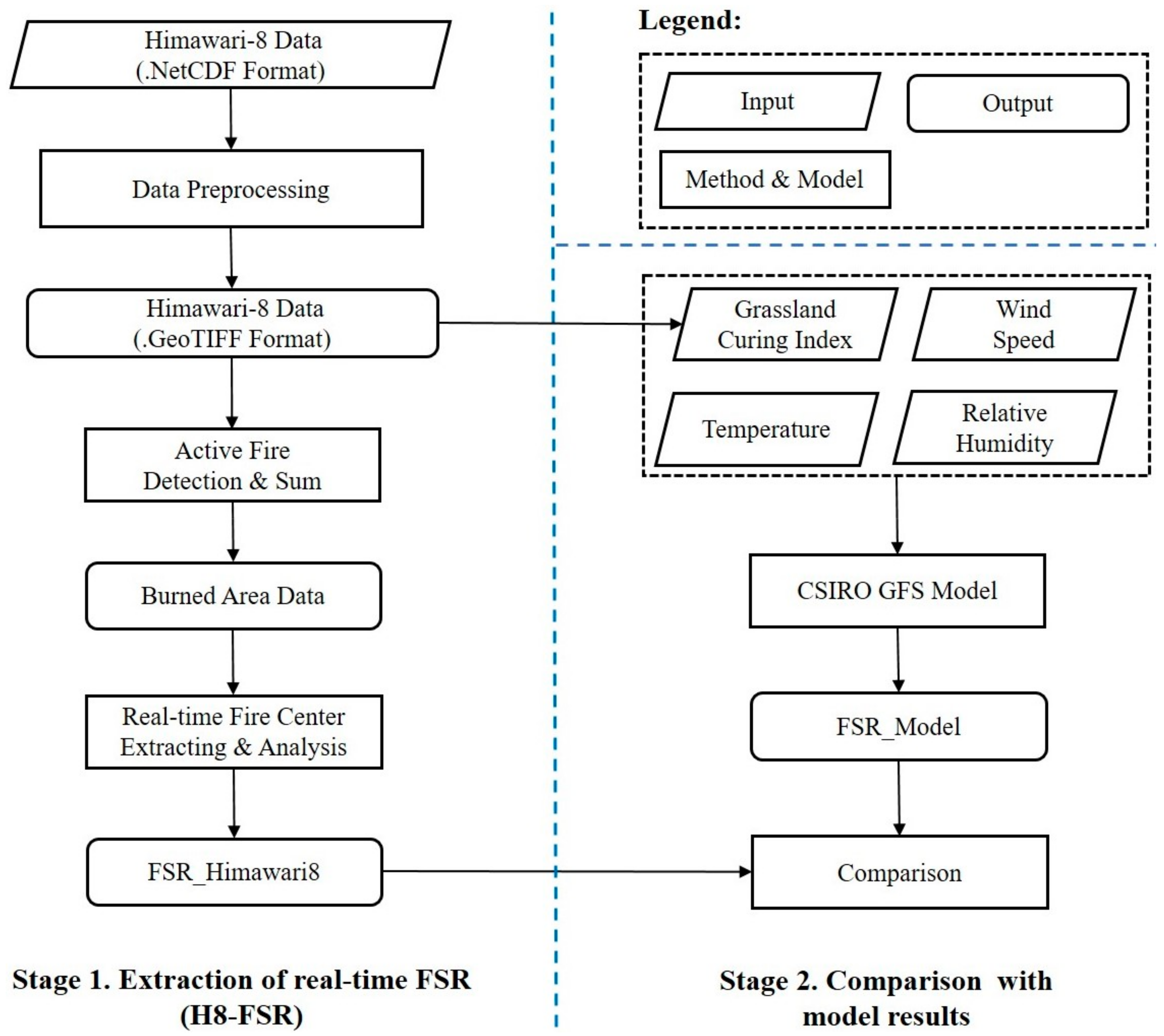
The methodology in this study can be divided into two stages (see Figure 2): (i) The extraction of near real-time FSR (H8-FSR), consisting of data preprocessing, near real-time burned area detection, near real-time fire center extraction, and near real-time FSR calculation; and (ii) The comparison of H8-FSR results with those obtained using the CSIRO GFS Model.

3.1. Data Preprocessing

The Himawari-8 data downloaded from the JAXA were in the ‘NetCDF’ format, therefore, data preprocessing was needed prior to operational use. This included converting the format, writing geographic information, clipping and re-projecting onto the Geocentric Datum of Australia (GDA) 1994 South Australia Lambert coordinates.

3.2. Near Real-Time Burned Area Detection

In this study, the burned area data were identified based on each Himawari-8 image using Equation (1). From this equation, the burned area data at timestamp i equates to the sum of the active fire data in the past two hours. The two-hour interval was found to be suitable for the area chosen in this study. However, the suitability of this time interval should be explored further, if applied to other wildfires. The active fire detection algorithm developed by Xu et al. [46] was used to detect the Esperance wildfire. The algorithm was modified from the active fire detection algorithm used in the MOD64 collection 6 product [52]. This modification is based on a certain threshold required to detect a possible active fire and then eliminating any false positives (e.g., water and cloud masking). The pixels that match the Equation (3) are classified as active fire. The empirical thresholds used in Equation (2) were specifically adjusted for the case study.
B A i = A F i A F i - 1 A F i - 12  
( a b s ( A 0.64 ) < 0.01 ) ( a b s ( A 0.86 ) < 0.01 ) : n i g h t - t i m e ( T 3.9 m e a n ( T 3.9 ) s t d ( T 3.9 ) > 0.8 ) ( T 3.9 m e a n ( T 3.9 ) s t d ( T 3.9 ) T 11.2 m e a n ( T 11.2 ) s t d ( T 11.2 ) > 1.5 ) : p o s s i b l e - A F A 2.3 > 0.05 : n o t - w a t e r ( A 0.64 + A 0.86 < 1.2 ) ( T 12.4 < 265 K ) ( ( A 0.64 + A 0.86 < 0.7 ) ( T 12.4 > 285 K ) ) : n o t - c l o u d
p o s s i b l e - A F n o t - w a t e r n o t - c l o u d : A F p o s s i b l e - A F n i g h t - t i m e : A F
where BA and AF represent burned area and active fire, respectively. A0.64 denotes the albedo value at 0.64 µm, T3.9 denotes the brightness temperature value at 3.9 µm, mean(T3.9) and std(T3.9) denote the average and standard deviation of T3.9 within the study area.

3.3. Near Real-Time Fire Center Extraction

In this study, the centroid of the burned area was defined as the fire center. The centroid of a target is one of the most useful measurements for describing the spatial distribution of a target [53,54,55,56]. Therefore, the centroid of the burned area can represent the average location of a fire at any time stamp. After obtaining the burned area data (see Section 3.2), Equation (4) was applied together with R software [57] to extract the geographical coordinates of each fire center.
X c = i = 1 n m i x i i = 1 n m i , Y c = i = 1 n m i y i i = 1 n m i  
where Xc and Yc are the geographical coordinates of the fire center, n is the number of pixels flagged burned, xi and yi are the geographical coordinates of the i-th pixel, and mi is the area of the i-th pixel.

3.4. Near Real-Time FSR Calculation

Himawari-8 provides an observation every 10 minutes, which makes it possible to retrieve FSR at near real-time by analyzing the spread progression of the fire center. Wildfire spread models that are based on Huygens’ wavelet principle presume that there is an elliptical spread at each point of the fire-front, and that a fire spreads outwards elliptically and at a constant speed in windless and flat area conditions [58,59,60,61,62,63]. Therefore, it can be assumed that the FSR can be represented by the rate of burned area centroid movement in a windy environment. Additionally, fire spread models define the fire spread direction (FSD) as the reverse of wind direction [23]. The wind direction is generally expressed in 16 directions on the land with an average of 22.5 degrees [64]. Following these principles, the azimuth of centroid movement (αi, also called FSD) from time stamp i − 1 to i is first calculated using Equation (5), and then the difference (△) between the azimuth of centroid movement and reverse wind direction (RWD) is calculated (Equation (6)).
α i = arctan Y c t i Y c t i 1 X c t i X c t i 1  
Δ = | α i ( D R W i n d ± 180 ) |  
where X c t i , Y c t i , X c t i + 1 , and Y c t i + 1 are the geographical coordinates of the burned area centroid in time stamp i and i + 1, D R W i n d is the reverse wind direction.
Finally, the near real-time FSR, corresponding to △ lower than 22.5 degrees, is calculated at different timesteps using Equation (7).
V ( i 1 , i ) = D ( i 1 , i ) T r  
where T r is the time resolution of Himawari-8, V ( i 1 , i ) is the FSR during the timestep i − 1 to i, D ( i 1 , i ) is the distance of the centroid movement during timestep i − 1 to i. D ( i 1 , i ) can be obtained with Equation (8).
D ( i 1 , i ) = ( X c t i 1 X c t i ) 2 + ( Y c t i 1 Y c t i ) 2  

3.5. Comparison of Results with the CSIRO GFS Model

The FSR computed from the CSIRO GFS model [27] was used as a benchmark to assess the performance of H8-FSR. The CSIRO GFS model was calibrated using 121 experimental fires and 20 major wildfires in Australia [65]. This model is broadly used by the Australian fire authorities [65]. The inputs of the model include meteorological information (10 m open wind speed, temperature, relative humidity) as well as a Grassland curing index (GCI). In this study, the meteorological data was obtained from three stations as described in Section 2.3. GCI, defined as the percentage of dead materials over the grass sward, has a large influence on grassland fire propagation [66]. To date, there are two GCI satellite-based products for Australia, with a time and spatial resolution of eight days and 500 m respectively. The GCI product developed by Martin et al. [67] is more accurate than the curing product developed by Newnham et al. [68]. The algorithm developed by Martin et al. [67] retrieves GCI using the Normalized Difference Vegetation Index (NDVI) and the Global Vegetation Monitoring Index (GVMI) computed from three window bands of MODIS (MOD09A1) satellite data, centered at 0.64 µm (band 1), 0.86 µm (band 2) and 1.64 µm (band 6). The algorithm was trained on curing visual estimates obtained by following the Australia Country Fire Authority (CFA) guide [67]. Therefore, GCI was eventually obtained by applying this algorithm to the Himawari-8 data acquired from the Esperance bushfire that broke out at AWST time 08:30.
FSR derived from the CSIRO GFS model and the H8-FSR were compared using the coefficient of determination (R2), the mean bias error (MBE) (Equation (9)), the mean absolute percent error (MAPE) (Equation (10)) and the root mean square error (RMSE) (Equation (11)) [69].
M B E = ( V H 8 V M ) n  
M A P E = ( V H 8 V M V M ) n 100  
R M S E = ( V H 8 V M ) 2 n  
where VH−8 is the FSR extracted from THE Himawari-8 data, VM is the FSR estimated from the CSIRO GFS model and n is the number of observations.

4. Results

4.1. Burned Area Variation

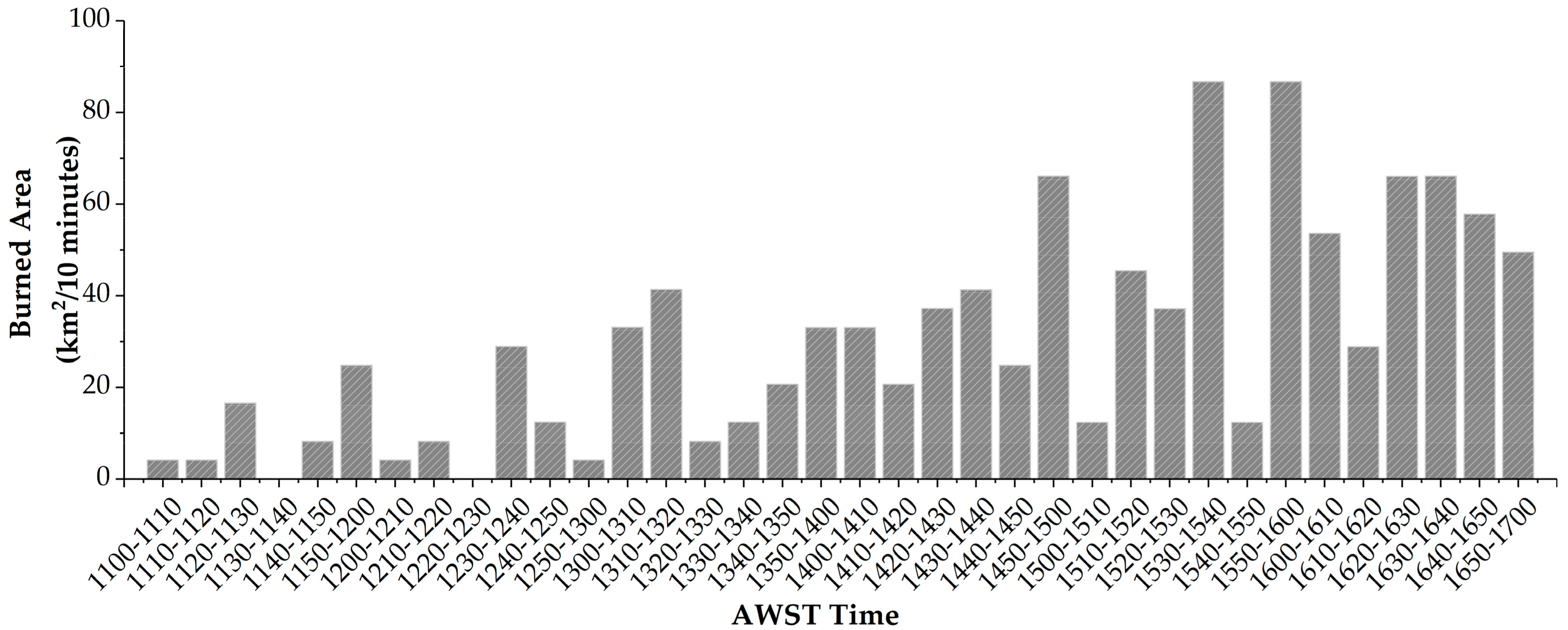
The total burned area obtained from the Himawari-8 for fire event that was studied (6 h, 10 min time periods) was 1090.62 km2. The variation in the burned area fluctuated from 0 km2/10 min (11:30–11:40 and 12:20–12:30 periods) to 41.35 km2/10 min (13:10–13:20 period) before 13:20 AWST with an average rate of (13.44 km2/10 min) (Figure 3). However, it rapidly increased thereafter, achieving a peak value close to 90 km2/10 min at AWST 15:30–15:40 and 15:50–16:00 (Figure 3).

4.2. Near Real-Time FSR

Using Equation (3), the difference between the FSD and the RWD for Esperance wildfire (36 time periods) were calculated. The number of time periods falling in different difference intervals were counted (Table 1). The FSR of 30 time periods with differences (△) lower than 22.5 degrees were calculated in three directions. The extracted direction was FSD and the south and east directions were calculated by decomposing wind speed.
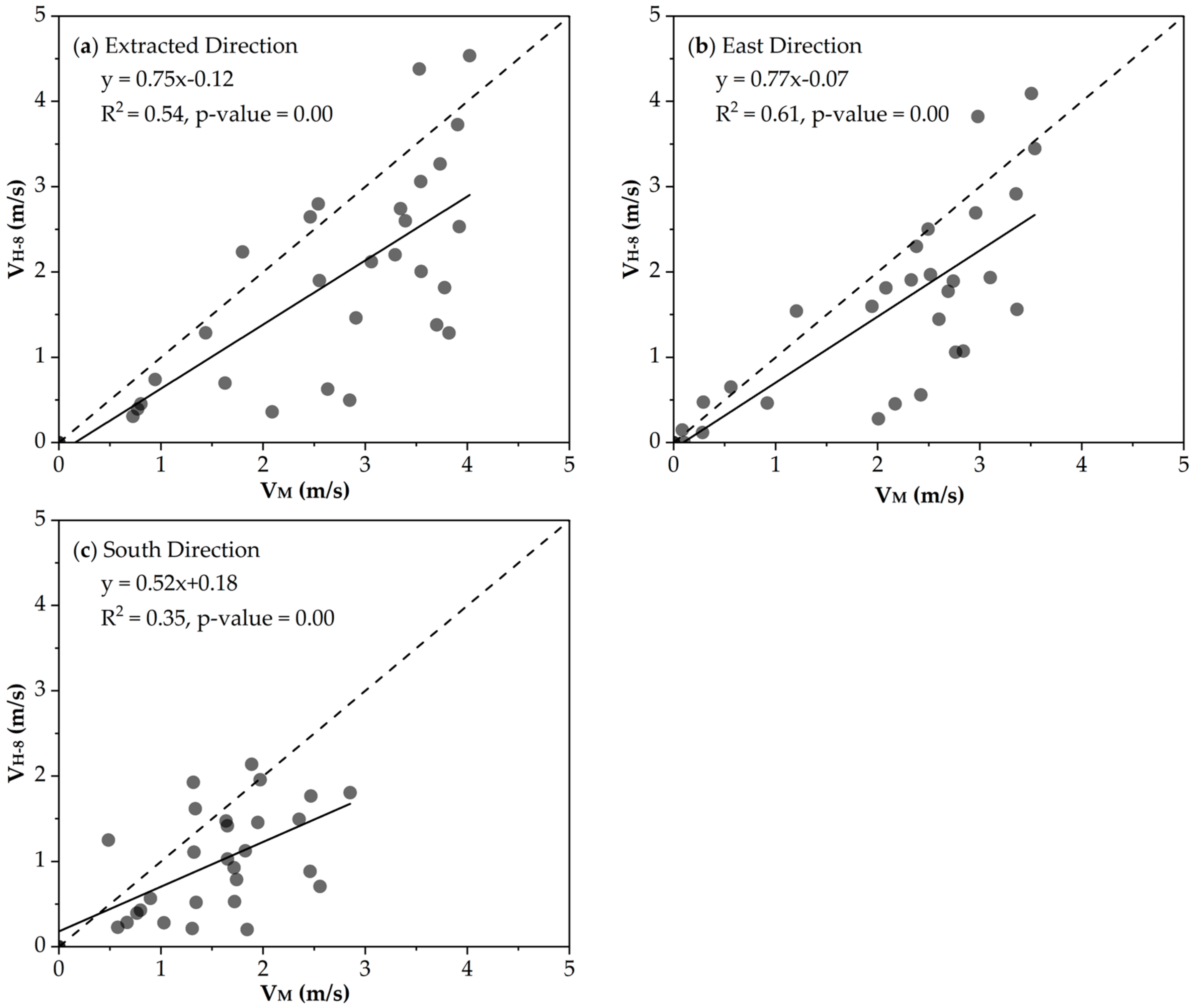
Compared with the CSIRO GFS model, the H8-FSR under-estimated the FSR in the south, east and extracted directions (MBE = −0.52 m/s, −0.52 m/s and −0.75 m/s, respectively) (Table 2) with a MAPE of 43.33%, 35.53% and 33.20% (Table 2). The statistical metrics demonstrated a better agreement between the model estimates in the east and extracted directions compared to the south direction (Table 2 and Figure 4). The south direction demonstrated a larger MAPE (43.33%), a smaller R2 (0.35) and a regression line that deviated from the 1:1 ideal line. However, the RMSE (0.80 m/s) was found to be smaller than the RMSE of the other two directions. Figure 4c demonstrates a less scattered distribution of dots, while the maximum FSR extracted from the Himawari-8 data (2.2 m/s) in the south direction was smaller than the FSR extracted from Himawari-8 data in the east and extracted directions. These may account for the low RMSE value.
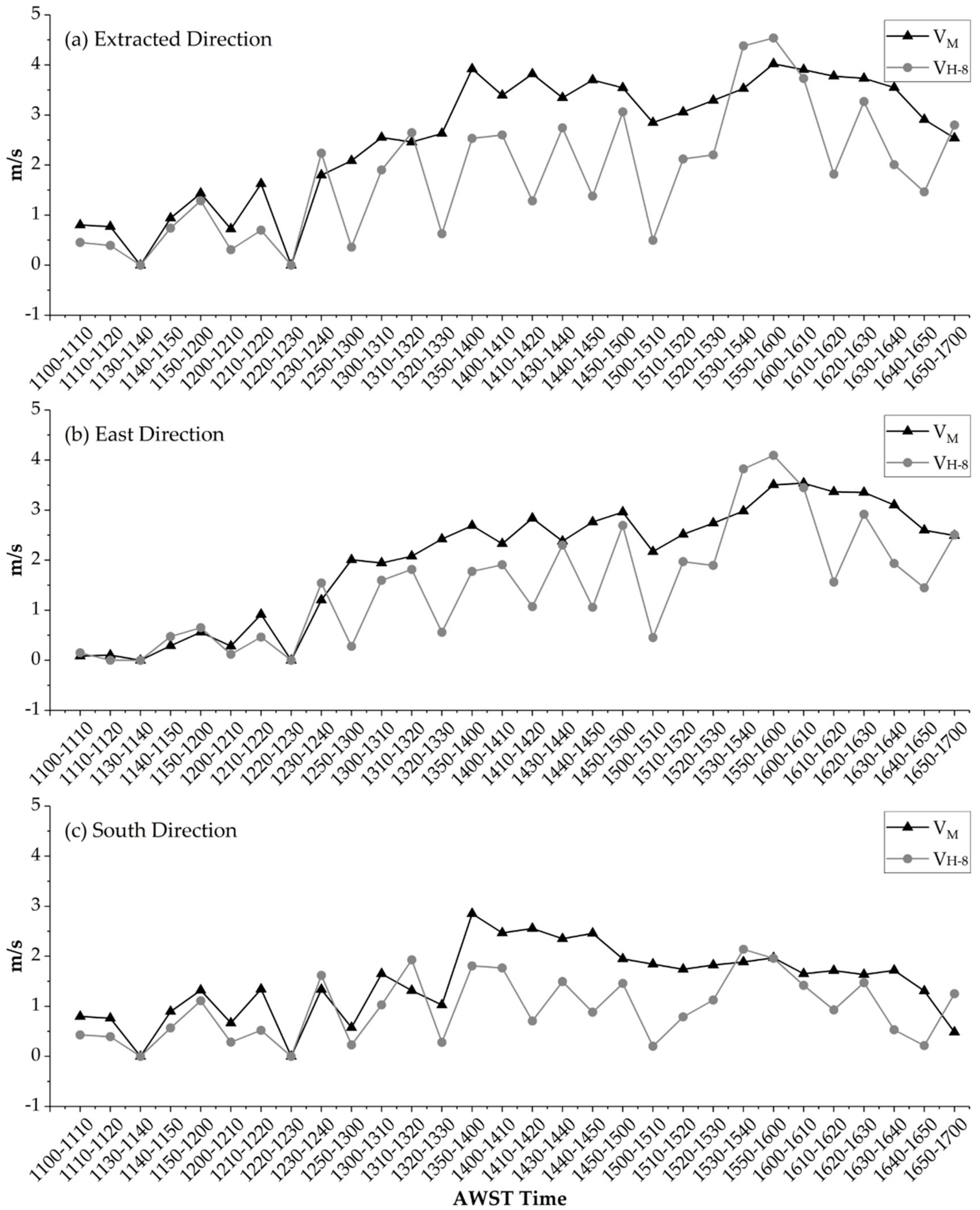
Figure 5 indicates that the FSR extracted from the Himawari-8 data is very close to the FSR estimated from the CSIRO GFS model for the 10-min time period from 11:00 to 12:40, especially in the east direction (Figure 5b). A large deviation occurs from 12:50 to 15:10 when CSIRO GFS model generally obtains higher FSR. However, the FSR derived from the Himawari-8 data is higher than the FSR estimated from the CSIRO GFS model at 15:30−15:40 and 15:50−16:00 periods.

5. Discussion

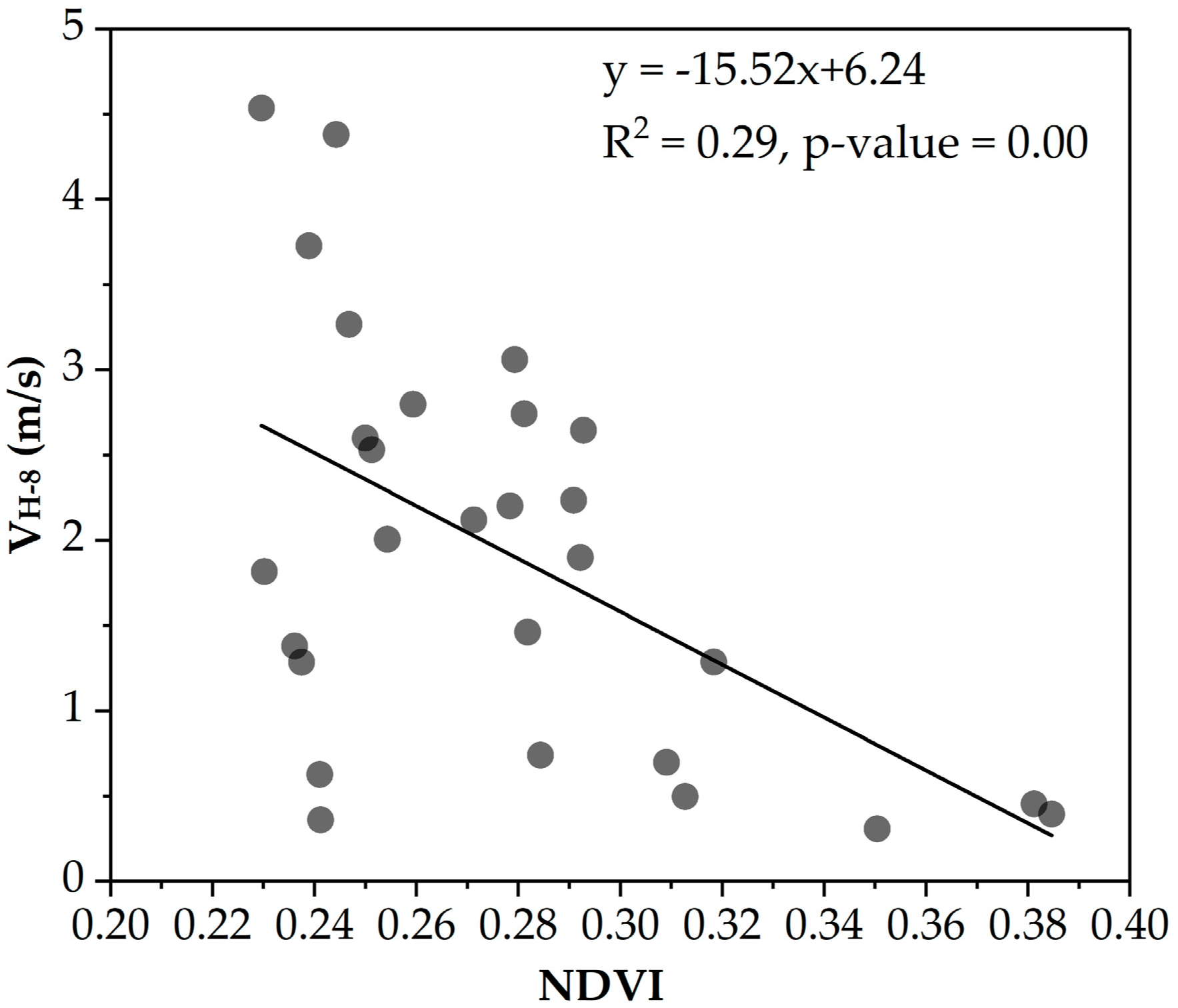
This is the first study to evaluate the performance of near real-time FSR extraction from the Himawari-8 data. The FSR estimated from the CSIRO GFS model was used as a benchmark to compare and assess the performance of H8-FSR. The H8-FSR compared favorably to the CSIRO GFS model when it came to the extraction of the near real-time FSR in the Esperance wildfire and produced errors that were acceptable within the literature (~30% MAPE [28]). However, H8-FSR underestimated FSR in some instances. These underestimations may have been the result of several reasons. Firstly, the CSIRO GFS model may have overestimated the FSR because this model assumes a fire will not be constrained during its growth [70]. Additionally, the CSIRO GFS model does not take into account topography. However, weather, fuel and topography together are the key factors affecting fire behavior [71]. Nevertheless, Esperance, the site that was studied is very flat and hence, the effect of topography may be insignificant. Another potential reason for the underestimations may have arisen from the meteorological information that was used. The meteorological information was calculated from the average values obtained from three different meteorological stations. For example, the wind speed and relative humidity values reported by the three stations highly differed at certain time periods (13:20–13:30, 14:10–14:20, 14:40–14:50, and 15:00–15:10), coinciding with the time periods where the FSR estimated with H8-FSR and CSRO GFS model differed the most (Figure 5). Using values for the average wind speed and relative humidity for the data recorded at the three meteorological stations as inputs to the CSIRO GFS model may have led to the observed deviations. On the other hand, fuel moisture content (FMC), including live and deal fuels moisture content, has proven to be a key indicator for fire risk assessment and FSR prediction [72,73,74,75]. However, the CSIRO GFS model only considers the dead FMC, which is derived from meteorological factors [27]. In recent years, several studies have propagated for the use of remote sensing data to retrieve FMC and indeed, this has achieved reasonable results [75,76,77,78]. Therefore, further work will focus on applying the method to the Himawari-8 data to retrieve near real-time live and dead FMC and using those estimates as input parameters for fire behavior and risk assessments. Moreover, different vegetation types and growth conditions may also affect the FSR. The NDVI of the vegetation near the Esperance bushfire that ignited (at AWST time 08:30) was also computed from the Himawari-8 data, and then the NDVI of the burned area which increased at different timesteps were eventually extracted. The relationship between the NDVI and the FSR is shown in Figure 6. The FSR is faster in the area with lower NDVI. In contrast, when the NDVI is higher, which means the vegetation is very lush and difficult to ignite [79], the FSR becomes smaller. In this study, the region that was selected for this research was dominated by grassland but also comprised of little crops and shrubs. Consequently, this may also affect the evaluation of H8-FSR since the benchmark model was constructed within the context of grassland and without accounting for other vegetation types.
The H8-FSR also has certain limitations. Firstly, it was assumed that the centroid of the burned area represented the average location of the fire, thus, the burned area data formed the base of FSR extraction. The FSR extracted from the Himawari-8 data was small at the time periods 12:50–13:00, 13:20–13:30 and 15:00–15:10 (Figure 5). As a result, the rate of burned area growth was also small. Therefore, the inaccuracy of burned area data affects the precision of the H8-FSR. The spatial resolution (2 km) of the Himawari-8 data is still not adequate enough, and this may introduce challenges to the detection of mixed pixels with different degrees of combustion. Unfortunately, at present, there is no officially reliable Himawari-8 burned area product. In this study, the sum of the active fire data was used to get the burned area data. The active fire detection algorithm is based on certain thresholds, which may not be robust for different regions. Therefore, in order to better apply the Himawari-8 data to fire research, it is necessary to develop a reliable product of burned extend for Himawari-8 fire. The second important limitation of H8-FSR is that it estimates an overall distribution of FSR by computing the rate of burned area centroid movement in a windy climate. The rate of fire center movement can well represent overall FSR when all the pixels have a similar direction of movement at every time step. However, small-scale wind has a substantial direction variation [80,81], which means the burned pixels in varying locations have different directions when the wind speed is very small. As a result, the movement of a fire center cannot actually reflect the fire spread, and thus affects the effectiveness of the H8-FSR.

6. Conclusions

The spatial-temporal distribution of the FSR is vital for fire management; for example, the establishment of firebreaks and the evacuation of personnel. The near real-time FSR extracted from the Himawari-8 data can provide more information for fire agencies in predicting the location of fire propagation. This in turn could lead to improvements in the efficiency of operational firefighting. This paper first defined the fire center as the burned area centroid and then proposed a novel method for near real-time FSR extraction based on the movement rate of the fire center which is extracted from the high-temporal resolution Himawari-8 data. The methodology was applied to a wildfire case that occurred in Esperance, Western Australia on 17 November, 2015. The results demonstrated that the H8-FSR could extract the FSR from Himawari-8 data well, compared with the CSIRO GFS model. The accuracy of burned area extraction and the scale of wind may also affect the efficacy of H8-FSR, which was discussed in Section 5 and remains to be investigated further. Further improvement in terms of the H8-FSR and its application to other vegetation types such as forest and shrubland, and testing the H8-FSR with other geostationary satellites needs to be implemented. Such satellites could include GaoFen-4 (GF-4), Feng Yun-4 (FY-4), GEO-R and Next Geostationary Korea multipurpose Satellite-2A (GK-2A). This would serve to improve the development of a global geostationary fire observation and prevention system.

Author Contributions

X.L., B.H., and X.Q. conceived and designed the experiments; X.L., S.Q., C.Y., Z.L. and H.Z. performed the experiments; and X.L., X.Q., and M.Y. analyzed the data and wrote the paper. All of the authors contributed to the editing of the manuscript.

Funding

This work was supported by the National Natural Science Foundation of China (Contract No. 41671361 and 41601373 and 41801272), the Fundamental Research Fund for the Central Universities (Contract No. ZYGX2017KYQD195).

Acknowledgments

The authors would like to thank the JAXA for providing the Himawari-8 data, as well as the Australian Bureau of Meteorology for contributing weather information.

Conflicts of Interest

The authors declare no conflicts of interest.

References

  1. Ruokolainen, L.; Salo, K. The effect of fire intensity on vegetation succession on a sub-xeric heath during ten years after wildfire. Ann. Bot. Fenn. 2009, 46, 30–42. [Google Scholar] [CrossRef]
  2. Bowman, D.M.; Balch, J.K.; Artaxo, P.; Bond, W.J.; Carlson, J.M.; Cochrane, M.A.; D’Antonio, C.M.; Defries, R.S.; Doyle, J.C.; Harrison, S.P.; et al. Fire in the earth system. Science 2009, 324, 481–484. [Google Scholar] [CrossRef] [PubMed]
  3. Chu, T.; Guo, X. Remote sensing techniques in monitoring post-fire effects and patterns of forest recovery in boreal forest regions: A review. Remote Sens. 2013, 6, 470–520. [Google Scholar] [CrossRef]
  4. Boerner, R.E.J.; Huang, J.; Hart, S.C. Impacts of fire and fire surrogate treatments on forest soil properties: A meta-analytical approach. Ecol. Appl. 2009, 19, 338–358. [Google Scholar] [CrossRef] [PubMed]
  5. Kilgore, B.M. The ecological role of fire in sierran conifer forests: Its application to national park management. Quat. Res. 1973, 3, 496–513. [Google Scholar] [CrossRef]
  6. Van der Werf, G.R.; Morton, D.C.; DeFries, R.S.; Olivier, J.G.J.; Kasibhatla, P.S.; Jackson, R.B.; Collatz, G.J.; Randerson, J.T. CO2 emissions from forest loss. Nat. Geosci. 2009, 2, 737–738. [Google Scholar] [CrossRef]
  7. Van der Werf, G.R.; Randerson, J.T.; Giglio, L.; Collatz, G.J.; Kasibhatla, P.S.; Arellano, A.F. Interannual variability in global biomass burning emissions from 1997 to 2004. Atmos. Chem. Phys. 2006, 6, 3423–3441. [Google Scholar] [CrossRef] [Green Version]
  8. Kochi, I.; Donovan, G.H.; Champ, P.A.; Loomis, J.B. The economic cost of adverse health effectsfrom wildfire-smoke exposure: A review. Int. J. Wildland Fire 2010, 19, 803–817. [Google Scholar] [CrossRef]
  9. Hesseln, H.; Loomis, J.B.; Gonzalez-Caban, A.; Alexander, S. Wildfire effects on hiking and biking demand in new mexico: A travel cost study. J. Environ. Manag. 2003, 69, 359–368. [Google Scholar] [CrossRef] [PubMed]
  10. Richardson, L.A.; Champ, P.A.; Loomis, J.B. The hidden cost of wildfires: Economic valuation of health effects of wildfire smoke exposure in southern california. J. For. Econ. 2012, 18, 14–35. [Google Scholar] [CrossRef]
  11. Doerr, S.H.; Santin, C. Global trends in wildfire and its impacts: Perceptions versus realities in a changing world. Philos. Trans. R. Soc. Biol. Sci. 2016, 371. [Google Scholar] [CrossRef] [PubMed]
  12. Johnston, F.H.; Henderson, S.B.; Chen, Y.; Randerson, J.T.; Marlier, M.; Defries, R.S.; Kinney, P.; Bowman, D.M.; Brauer, M. Estimated global mortality attributable to smoke from landscape fires. Environ. Health Perspect. 2012, 120, 695–701. [Google Scholar] [CrossRef] [PubMed]
  13. Cruz, M.G.; Gould, J.S.; Alexander, M.E.; Sullivan, A.L.; McCaw, W.L.; Matthews, S. Empirical-based models for predicting head-fire rate of spread in australian fuel types. Aust. For. 2015, 78, 118–158. [Google Scholar] [CrossRef]
  14. Rossa, C.G.; Fernandes, P.M. Fuel-related fire-behaviour relationships for mixed live and dead fuels burned in the laboratory. Can. J. For. Res. 2017, 47, 883–889. [Google Scholar] [CrossRef] [Green Version]
  15. Cruz, M.G.; Alexander, M.E.; Sullivan, A.L.; Gould, J.S.; Kilinc, M. Assessing improvements in models used to operationally predict wildland fire rate of spread. Environ. Model. Softw. 2018, 105, 54–63. [Google Scholar] [CrossRef]
  16. Cheney, N.P.; Gould, J.S.; McCaw, W.L.; Anderson, W.R. Predicting fire behaviour in dry eucalypt forest in southern Australia. For. Ecol. Manag. 2012, 280, 120–131. [Google Scholar] [CrossRef]
  17. Jenkins, M.J.; Page, W.G.; Hebertson, E.G.; Alexander, M.E. Fuels and fire behavior dynamics in bark beetle-attacked forests in western north america and implications for fire management. For. Ecol. Manag. 2012, 275, 23–34. [Google Scholar] [CrossRef]
  18. Cruz, M.G.; Alexander, M.E. Modelling the rate of fire spread and uncertainty associated with the onset and propagation of crown fires in conifer forest stands. Int. J. Wildland Fire 2017, 26, 413–426. [Google Scholar]
  19. Benali, A.A.; Pereira, J.M.C. Monitoring and extracting relevant parameters of wild fire spread using remote sensing data. In Proceedings of the Anais XVI Simpósio Brasileiro de Sensoriamento Remoto-SBSR, Foz do Iguaçu, PR, Brasil, 13–18 April 2013. [Google Scholar]
  20. Gould, J.S.; Sullivan, A.L.; Hurley, R.; Koul, V. Comparison of three methods to quantify the fire spread rate in laboratory experiments. Int. J. Wildland Fire 2017, 26, 877. [Google Scholar] [CrossRef]
  21. Sullivan, A.L. Wildland surface fire spread modelling, 1990–2007. 1: Physical and quasi-physical models. Int. J. Wildland Fire 2009, 18, 349–368. [Google Scholar] [CrossRef]
  22. Sullivan, A.L. Wildland surface fire spread modelling, 1990–2007. 2: Empirical and quasi-empirical models. Int. J. Wildland Fire 2009, 18, 369–386. [Google Scholar] [CrossRef]
  23. Plucinski, M.P.; Sullivan, A.L.; Rucinski, C.J.; Prakash, M. Improving the reliability and utility of operational bushfire behaviour predictions in australian vegetation. Environ. Model. Softw. 2017, 91, 1–12. [Google Scholar] [CrossRef]
  24. Rothermel, R.C. A Mathematical Model for Predicting Fire Spread in Wildland Fuels; USDA Forest Service Research Paper INT-115; U.S. Department of Agriculture, Forest Service, Intermountain Forest and Range Experiment Station: Ogden, UT, USA, 1972. [Google Scholar]
  25. Lawson, B.D.; Stocks, B.J.; Alexander, M.E.; Van Wagner, C.E. A system for predicting fire behavior in canadian forests. In Proceedings of the 8th Conference on Fire and Forest Meteorology, Detroit, MI, USA, 29 April–2 May 1985. [Google Scholar]
  26. McArthur, A.G. Fire Behavior in Eucalypt Forests; Department of National Development, Forestry and Timber Bureau Leaflet: Canberra, Australia, 1967. [Google Scholar]
  27. Cheney, N.P.; Gould, J.S.; Catchpole, W.R. Prediction of fire spread in grasslands. Int. J. Wildland Fire 1998, 8, 1–13. [Google Scholar] [CrossRef]
  28. Cruz, M.G.; Alexander, M.E. Uncertainty associated with model predictions of surface and crown fire rates of spread. Environ. Model. Softw. 2013, 47, 16–28. [Google Scholar] [CrossRef]
  29. Linn, R.; Reisner, J.; Colman, J.J.; Winterkamp, J. Studying wildfire behavior using firetec. Int. J. Wildland Fire 2002, 11, 233. [Google Scholar] [CrossRef]
  30. Lymberopoulos, N.; Tryfonopoulos, T.; Lockwood, F. The study of small and meso-scale wind field-forest fire interaction and buoyancy effects using the aiolos-f simulator. In Proceedings of the III International Conference on Forest Fire Research, 14th Conference on Fire and Forest Meteorology, Luso, Portugal, 16–20 November 1998. [Google Scholar]
  31. Morvan, D.; Larini, M. Modeling of one dimensional fire spread in pine needles with opposing air flow. Combust. Sci. Technol. 2001, 164, 37–64. [Google Scholar] [CrossRef]
  32. Mell, W.; Jenkins, M.A.; Gould, J.; Cheney, P. A physics-based approach to modelling grassland fires. Int. J. Wildland Fire 2007, 16, 1–22. [Google Scholar] [CrossRef]
  33. Cruz, M.G.; Kidnie, S.; Matthews, S.; Hurley, R.J.; Slijepcevic, A.; Nichols, D.; Gould, J.S. Evaluation of the predictive capacity of dead fuel moisture models for eastern australia grasslands. Int. J. Wildland Fire 2016, 25, 995–1001. [Google Scholar] [CrossRef]
  34. Stow, D.A.; Riggan, P.J.; Storey, E.J.; Coulter, L.L. Measuring fire spread rates from repeat pass airborne thermal infrared imagery. Remote Sens. Lett. 2014, 5, 803–812. [Google Scholar] [CrossRef]
  35. Loboda, T.V.; Csiszar, I.A. Reconstruction of fire spread within wildland fire events in northern eurasia from the modis active fire product. Glob. Planet. Chang. 2007, 56, 258–273. [Google Scholar] [CrossRef]
  36. Sifakis, N.I.; Iossifidis, C.; Kontoes, C.; Keramitsoglou, I. Wildfire detection and tracking over greece using msg-seviri satellite data. Remote Sens. 2011, 3, 524–538. [Google Scholar] [CrossRef]
  37. Hally, B.; Wallace, L.; Reinke, K.; Jones, S. Assessment of the utility of the advanced himawari imager to detect active fire over Australia. In Proceedings of the XXIII ISPRS Congress, Prague, Czech Republic, 12–19 July 2016. [Google Scholar]
  38. Zhang, X.; Kondragunta, S.; Ram, J.; Schmidt, C.; Huang, H.-C. Near-real-time global biomass burning emissions product from geostationary satellite constellation. J. Geophys. Res. Atmos. 2012, 117, 1–18. [Google Scholar] [CrossRef]
  39. Zhang, X.; Kondragunta, S. Temporal and spatial variability in biomass burned areas across the USA derived from the goes fire product. Remote Sens. Environ. 2008, 112, 2886–2897. [Google Scholar] [CrossRef]
  40. Calle, A.; Casanova, J.L.; Romo, A. Fire detection and monitoring using msg spinning enhanced visible and infrared imager (seviri) data. J.Geophys. Res. Biogeosci. 2006, 111. [Google Scholar] [CrossRef]
  41. Laneve, G.; Castronuovo, M.M.; Cadau, E.G. Continuous monitoring of forest fires in the mediterranean area using msg. IEEE Trans. Geosci. Remote Sens. 2006, 44, 2761–2768. [Google Scholar] [CrossRef]
  42. Kim, G.; Kim, D.-S.; Park, K.-W.; Cho, J.; Han, K.-S.; Lee, Y.-W. Detecting wildfires with the korean geostationary meteorological satellite. Remote Sens. Lett. 2014, 5, 19–26. [Google Scholar] [CrossRef]
  43. Da, C. Preliminary assessment of the advanced himawari imager (ahi) measurement onboard himawari-8 geostationary satellite. Remote Sens. Lett. 2015, 6, 637–646. [Google Scholar] [CrossRef]
  44. Fatkhuroyan; Wati, T.; Panjaitan, A. Forest fires detection in indonesia using satellite himawari-8 (case study: Sumatera and kalimantan on august-october 2015). IOP Conf. Ser. Earth Environ. Sci. 2017, 54. [Google Scholar] [CrossRef]
  45. Sataid Software. Available online: https://www.data.jma.go.jp/mscweb/en/VRL/sataid/program.html (accessed on 16 October 2018).
  46. Xu, G.; Zhong, X. Real-time wildfire detection and tracking in australia using geostationary satellite: Himawari-8. Remote Sens. Lett. 2017, 8, 1052–1061. [Google Scholar] [CrossRef]
  47. Xu, W.; Wooster, M.J.; Kaneko, T.; He, J.; Zhang, T.; Fisher, D. Major advances in geostationary fire radiative power (frp) retrieval over asia and australia stemming from use of himarawi-8 ahi. Remote Sens. Environ. 2017, 193, 138–149. [Google Scholar] [CrossRef]
  48. Wickramasinghe, C.; Jones, S.; Reinke, K.; Wallace, L. Development of a multi-spatial resolution approach to the surveillance of active fire lines using himawari-8. Remote Sens. 2016, 8, 932. [Google Scholar] [CrossRef]
  49. Bessho, K.; Date, K.; Hayashi, M.; Ikeda, A.; Imai, T.; Inoue, H.; Kumagai, Y.; Miyakawa, T.; Murata, H.; Ohno, T.; et al. An introduction to himawari-8/9-japan’s new-generation geostationary meteorological satellites. J. Meteorol. Soc. Jpn. 2016, 94, 151–183. [Google Scholar] [CrossRef]
  50. JAXA Website. Available online: http://www.eorc.jaxa.jp/ptree/ (accessed on 16 October 2018).
  51. Australian Bureau of Meteorology Website. Available online: http://reg.bom.gov.au (accessed on 16 October 2018).
  52. Giglio, L.; Schroeder, W.; Justice, C.O. The collection 6 modis active fire detection algorithm and fire products. Remote Sens. Environ. 2016, 178, 31–41. [Google Scholar] [CrossRef] [PubMed]
  53. Rocchini, D.; Cateni, C. On the measure of spatial centroid in geography. Asian J. Inf. Technol. 2006, 5, 729–731. [Google Scholar]
  54. Bourke, P. Calculating the Area and Centroid of a Polygon. Available online: https://www.seas.upenn.edu/~sys502/extra_materials/Polygon%20Area%20and%20Centroid.pdf (accessed on 16 October 2018).
  55. Deakin, R.E.; Bird, S.C.; Grenfell, R.I. The centroid? Where would you like it to be be? Cartography 2002, 31, 153–167. [Google Scholar] [CrossRef]
  56. De Smith, M.J.; Goodchild, M.F.; Longley, P. Geospatial Analysis: A Comprehensive Guide to Principles, Techniques and Software Tools; Troubador Publishing Ltd.: Leicester, UK, 2007. [Google Scholar]
  57. Richards, G.D. A general mathematical framework for modeling two-dimensional wildland fire spread. Int. J. Wildland Fire 1995, 5, 63–72. [Google Scholar] [CrossRef]
  58. Rios, O.; Jahn, W.; Rein, G. Forecasting wind-driven wildfires using an inverse modelling approach. Nat. Hazards Earth Syst. Sci. 2014, 14, 1491–1503. [Google Scholar] [CrossRef] [Green Version]
  59. R software v3.4.1. Available online: https://cran.r-project.org/bin/windows/base/old/3.4.1/ (accessed on 16 October 2018).
  60. Glasa, J.; Halada, L. On elliptical model for forest fire spread modeling and simulation. Math. Comput. Simul. 2008, 78, 76–88. [Google Scholar] [CrossRef]
  61. Anderson, D.H.; Catchpole, E.A.; De Mestre, N.J.; Parkes, T. Modelling the spread of grass fires. J. Aust. Math. Soc. Ser. B Appl. Math. 1982, 23, 451–466. [Google Scholar] [CrossRef]
  62. Richards, G.D. An elliptical growth model of forest fire fronts and its numerical solution. Int. J. Numer. Methods Eng. 1990, 30, 1163–1179. [Google Scholar] [CrossRef]
  63. Richards, G.D. The properties of elliptical wildfire growth for time dependent fuel and meteorological conditions. Combust. Sci. Technol. 1993, 95, 357–383. [Google Scholar] [CrossRef]
  64. R software v3.4.1. Available online: https://www7.ncdc.noaa.gov/climvis/help_wind.html (accessed on 16 October 2018).
  65. Cruz, M.G.; Gould, J.S.; Alexander, M.E.; Sullivan, A.L.; McCaw, W.L.; Matthews, S. A Guide to Rate of Fire Spread Models for Australian Vegetation; Australasian Fire and Emergency Service Authorities Council Limited and Commonwealth Scientific and Industrial Research Organisation: Cabberra, ACT, Australia, 2015. [Google Scholar]
  66. Cruz, M.G.; Gould, J.S.; Kidnie, S.; Bessell, R.; Nichols, D.; Slijepcevic, A. Effects of curing on grassfires: Ii. Effect of grass senescence on the rate of fire spread. Int. J. Wildland Fire 2015, 24, 838–848. [Google Scholar] [CrossRef]
  67. Martin, D.; Chen, T.; Nichols, D.; Bessell, R.; Kidnie, S.; Alexander, J. Integrating ground and satellite-based observations to determine the degree of grassland curing. Int. J. Wildland Fire 2015, 24, 329–339. [Google Scholar] [CrossRef]
  68. Newnham, G.J.; Grant, I.F.; Martin, D.N.; Anderson, S.A. Improved Methods for Assessment and Prediction of Grassland Curing. Available online: http://www.bushfirecrc.com/publications/citation/bf-2555 (accessed on 16 October 2018).
  69. Willmott, C.J. Some comments on the evaluation of model performance. Bull. Am. Meteorol. Soc. 1982, 63, 1309–1313. [Google Scholar] [CrossRef]
  70. Sullivan, A.L. Grassland fire management in future climate. Adv. Agron. 2010, 106, 173–208. [Google Scholar]
  71. Pyne, S.J.; Andrews, P.L.; Laven, R.D. Introduction to Wildland Fire; John Wiley and Sons: New York, NY, USA, 1996. [Google Scholar]
  72. Rossa, C.G. The effect of fuel moisture content on the spread rate of forest fires in the absence of wind or slope. Int. J. Wildland Fire 2017, 26, 24–31. [Google Scholar] [CrossRef]
  73. Rossa, C.G.; Fernandes, P.M. Short communication: On the effect of live fuel moisture content on fire-spread rate. For. Syst. 2018, 26, eSC08. [Google Scholar] [CrossRef]
  74. Dasgupta, S.; Qu, J.; Hao, X.; Bhoi, S. Evaluating remotely sensed live fuel moisture estimations for fire behavior predictions in georgia, USA. Remote Sens. Environ. 2007, 108, 138–150. [Google Scholar] [CrossRef]
  75. Quan, X.; He, B.; Yebra, M.; Yin, C.; Liao, Z.; Li, X. Retrieval of forest fuel moisture content using a coupled radiative transfer model. Environ. Model. Softw. 2017, 95, 290–302. [Google Scholar] [CrossRef]
  76. Quan, X.W.; He, B.B.; Li, X.; Tang, Z. Estimation of grassland live fuel moisture content from ratio of canopy water content and foliage dry biomass. IEEE Geosci. Remote Sens. Lett. 2015, 12, 1903–1907. [Google Scholar] [CrossRef]
  77. Yebra, M.; Quan, X.; Riaño, D.; Rozas Larraondo, P.; van Dijk, A.I.J.M.; Cary, G.J. A fuel moisture content and flammability monitoring methodology for continental australia based on optical remote sensing. Remote Sens. Environ. 2018, 212, 260–272. [Google Scholar] [CrossRef]
  78. Yebra, M.; Dennison, P.E.; Chuvieco, E.; Riaño, D.; Zylstra, P.; Hunt, E.R.; Danson, F.M.; Qi, Y.; Jurdao, S. A global review of remote sensing of live fuel moisture content for fire danger assessment: Moving towards operational products. Remote Sens. Environ. 2013, 136, 455–468. [Google Scholar] [CrossRef]
  79. Quan, X.; He, B.; Yebra, M.; Yin, C.; Liao, Z.; Zhang, X.; Li, X. A radiative transfer model-based method for the estimation of grassland aboveground biomass. Int. J. Appl. Earth Obs. Geoinf. 2017, 54, 159–168. [Google Scholar] [CrossRef]
  80. Jiménez, P.A.; Dudhia, J. On the ability of the wrf model to reproduce the surface wind direction over complex terrain. J. Appl. Meteorol. Climatol. 2013, 52, 1610–1617. [Google Scholar] [CrossRef]
  81. Mahrt, L. Surface wind direction variability. J. Appl. Meteorol. Climatol. 2011, 50, 144–152. [Google Scholar] [CrossRef]
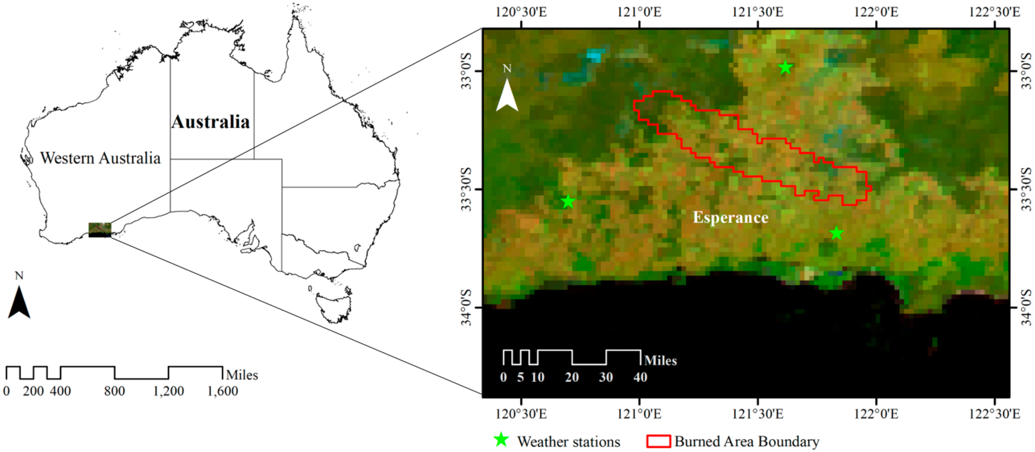
Figure 1. Location of the study area. The background is a pseudo-color composited Himawari-8 image (band 6, 4 and 3 corresponding to RGB) acquired at 8:30 a.m. Australia Western Standard Time (AWST) on 17 November 2015.
Remotesensing 10 01654 g001
Figure 2. A flowchart that demonstrates the methodology used in this study.
Remotesensing 10 01654 g002
Figure 3. Variation in the burned area at each period computed as the difference in burned area between two consecutive 10 min time periods.
Remotesensing 10 01654 g003
Figure 4. Scatterplots between the FSR extracted from Himawari-8 data (VH-8) and the CSIRO GFS model (VM) in three different directions. The short dash lines are 1:1 lines and the solid lines are linear regression lines.
Remotesensing 10 01654 g004
Figure 5. Time series of FSR extracted from the Himawari-8 data (VH-8) and the CSIRO GFS model (VM).
Remotesensing 10 01654 g005
Figure 6. Scatterplot showing the FSR extracted from the Himawari-8 data (VH-8) and the NDVI of different timesteps. The solid line indicates a linear regression.
Remotesensing 10 01654 g006
Table 1. Statistical summary of the differences between the FSD and RWD.
Difference△(°)
0–55–1010–1515–22.5>22.5
Number of time periods137646
% of Total36.1119.4416.6711.1616.67
Table 2. Quantitative comparison of the FSR extracted from Himawari-8 data and CSIRO GFS model. MBE, Mean Bias Error, MAPE, Mean Absolute Percent Error; RMSE, Root Mean Square Error and R2, coefficient of determination (*** p-Value = 0.00).
Extracted DirectionEast DirectionSouth Direction
MBE (m/s)−0.75−0.52−0.52
MAPE (%)33.2035.5343.33
RMSE (m/s)1.170.920.80
R20.54 ***0.61 ***0.35 ***