Article

Effects of Sample Plot Size and GPS Location Errors on Aboveground Biomass Estimates from LiDAR in Tropical Dry Forests

1
Centro de Investigación Científica de Yucatán A.C., Unidad de Recursos Naturales, Calle 43 # 130 , x 32 y 34 Colonia Chuburná de Hidalgo, Mérida CP 97205, Yucatán, Mexico
2
Laboratorio de Análisis de Información Geográfica y Estadística, El Colegio de la Frontera Sur, Carretera Panamericana y Periférico Sur s/n, San Cristóbal de las Casas CP 29290, Chiapas, Mexico
*
Author to whom correspondence should be addressed.
Remote Sens. 2018, 10(10), 1586; https://doi.org/10.3390/rs10101586
Submission received: 28 August 2018 / Revised: 18 September 2018 / Accepted: 29 September 2018 / Published: 2 October 2018
(This article belongs to the Section Forest Remote Sensing)

Abstract

:
Accurate estimates of above ground biomass (AGB) are needed for monitoring carbon in tropical forests. LiDAR data can provide precise AGB estimations because it can capture the horizontal and vertical structure of vegetation. However, the accuracy of AGB estimations from LiDAR is affected by a co-registration error between LiDAR data and field plots resulting in spatial discrepancies between LiDAR and field plot data. Here, we evaluated the impacts of plot location error and plot size on the accuracy of AGB estimations predicted from LiDAR data in two types of tropical dry forests in Yucatán, México. We sampled woody plants of three size classes in 29 nested plots (80 m2, 400 m2 and 1000 m2) in a semi-deciduous forest (Kiuic) and 28 plots in a semi-evergreen forest (FCP) and estimated AGB using local allometric equations. We calculated several LiDAR metrics from airborne data and used a Monte Carlo simulation approach to assess the influence of plot location errors (2 to 10 m) and plot size on ABG estimations from LiDAR using regression analysis. Our results showed that the precision of AGB estimations improved as plot size increased from 80 m2 to 1000 m2 (R2 = 0.33 to 0.75 and 0.23 to 0.67 for Kiuic and FCP respectively). We also found that increasing GPS location errors resulted in higher AGB estimation errors, especially in the smallest sample plots. In contrast, the largest plots showed consistently lower estimation errors that varied little with plot location error. We conclude that larger plots are less affected by co-registration error and vegetation conditions, highlighting the importance of selecting an appropriate plot size for field forest inventories used for estimating biomass.

1. Introduction

Tropical forests constitute a large proportion of the carbon stored in terrestrial ecosystems and play a crucial role in mitigating global climate change [1]. In particular, tropical dry forests (TDF) are the most extensive land cover type in the tropics and more than 50% of tropical dry forests are in the American continent [2]. However, forest conversion to other land uses exacerbates climate change; deforestation accounts for 15 to 25% of annual global greenhouse gas emissions [3]. Tropical dry forests (TDF) in particular combine high rates of deforestation with low coverage in protected areas [4]. Accurate estimations of aboveground biomass (AGB) are fundamental for climate change mitigation strategies such as REDD+ (Reducing Emissions from Deforestation and Degradation plus enhancing forest carbon stocks) and for establishing policies designed to maintain and enhance tropical forest carbon stocks.
Remote sensing is a valuable source of information to estimate and monitor AGB, because it offers an inexpensive means of attaining complete spatial coverage of information for large areas at regular time intervals [5]. Reflectance values and vegetation indices from passive optical satellite imagery have been used to estimate AGB in tropical forest [6]. However, these estimates are valid only for relatively young secondary forests as reflectance and vegetation indices saturate at the high biomass levels attained in older forests [7]. Another approach for AGB estimation is the use of Radar data. This active sensor has been used to estimate the spatial distribution of biomass [8], and also has the ability to penetrate clouds, one of the most important limitations in tropical regions. Nevertheless, as with the passive optical sensors, this sensor also shows limited sensitivity to biomass changes depending on the characteristics of the forest [9]. In contrast, LiDAR (Light Detection and Ranging) data can capture the horizontal and vertical structure of vegetation, which allows estimating AGB with a higher precision compared to approaches that used radar or optical data [10].
LiDAR is highly successful at estimating different vegetation attributes such as height, basal area, stem density, and AGB [11,12]. This active sensor uses laser pulses that have the ability to penetrate tropical forest canopies and detect three dimensional forest structures, allowing direct measurement of canopy height and providing three-dimensional canopy metrics that can be used to estimate forest vegetation structure parameters with no saturation at high biomass values [13,14]. Different studies have demonstrated a strong relationship between AGB and LiDAR measurements across all major forest ecosystems [14,15,16,17,18].
The most common approach to estimate the spatial distribution of AGB or carbon stocks from LiDAR data links data from field plots to LiDAR metrics from the same plots is through a statistical model. The model is then applied, together with LiDAR data, to predict biomass in un-sampled locations. Therefore, the accuracy of AGB estimations is directly influenced by the accuracy of co-registration of LiDAR data and field plots. However, consumer-grade GPS receivers, commonly used to locate plots in tropical forest inventories typically exhibit location errors that range from 2 to 10 m, depending on forest canopy conditions [19]. This means that LiDAR data and field plot data may not completely overlap spatially, potentially reducing the accuracy of predictions of forest AGB and carbon stocks. Some studies have assessed the influence of plot location errors on the precision of LiDAR based estimates of temperate forest structural parameters such as height, basal area, and volume [20], as well as biomass [21]. However, to our knowledge, the effect of errors in plot location on AGB estimations in tropical forest using LiDAR data has not been explored.
The precision of AGB estimations is also affected by plot size in two different ways. First, through edge effects, which occur when trees located outside of the plot boundary have large parts of their crowns inside the plot and/or trees located inside the plot have most of their crowns outside the plot. Since the perimeter to area ratio decreases as plot size increases, this edge effect should decrease with increasing plot size, resulting in greater overlap between plot data and LiDAR metrics data, and hence, in a higher precision of AGB estimates. Second, the spatial distribution of large trees, which make a disproportionally high contribution to stand AGB, is captured more accurately in larger plots than in smaller ones. As a result, large plots enable more precise estimations of AGB than small plots [22]. Moreover, the effects of plot size and plot location error may interact, since the area of overlap between LiDAR data and field plot data increases with plot size. Consequently, the effect of plot location error may decrease as plot size increases [20,23].
Finally, the effects of plot size and location error on the precision of AGB estimates from LiDAR data may vary with forest structural characteristics. Forest structural attributes, including stem density, basal area, and number of vertical strata among others, affect the spatial distribution of openings in the canopy, thereby potentially affecting the percentage of LiDAR returns that can be reflected by the canopy [23,24]. Consequently, the relationships between LiDAR metrics and vegetation structural parameters, such as canopy height, basal area, and AGB may vary with forest type or forest condition, as has been found in some studies [12,25]. This is important for estimating AGB at the regional level, where a range of different forest conditions or forest types usually occur.
The general goal of this research was to assess the impacts of plot location error and plot size on the accuracy of AGB estimations predicted from LiDAR data in two types of TDF that differ in vegetation structural complexity and species composition: a semi-deciduous forest with a less complex vegetation structure and lower diversity, compared to a semi-evergreen forest. To this end, five levels of plot location errors from 2 to 10 m at 2 m intervals and three plot sizes 80, 400 and 1000 m2 were considered. We predicted that: (1) the precision of LiDAR estimates of AGB would increase with sample plot size, reflecting decreasing edge effects and more accurate representation of large-sized trees. (2) The effect of sample plot location error on the precision of LIDAR estimates of AGB would decrease with plot size because of a higher degree of spatial overlap between sample plot and LiDAR data in larger plots. (3) The structurally more complex semi-evergreen forest, with a potentially lower percentage of LIDAR returns reflected by the canopy, would show a lower precision of AGB estimations from LiDAR and stronger effects of plot size and plot location error compared to the semi-deciduous forest.

2. Materials and Methods

2.1. Study Area

The study was conducted in two sites representing the most important tropical dry forest types of the Yucatan Peninsula (Figure 1). The Kaxil Kiuic site (Kiuic from now on) is located in the southern part of the State of Yucatan (20°04′N–20°06′N, 89°32′W–89°34′W) where vegetation is classified as seasonally dry semi-deciduous tropical forest (50–75% of species drop their leaves during the dry season). This forest has a relatively low canopy stature (13–18 m), with crown diameters (mean ± 1SD: 3.2 ± 1.6 m) and is dominated by Neomillspaughia emarginata, Gymnopodium floribundum, Bursera simaruba, Piscidia piscipula, and Lysiloma latisiliquum. The landscape consists of a mosaic of forest patches of different ages of abandonment after traditional slash-and-burn agriculture, agricultural fields, and small villages. The orography is characterized by hills of low elevation (60 to 180 m) and moderate slope (10–25°) alternating with plains. On the other hand, the Felipe Carrillo Puerto (FCP) site is situated in the State of Quintana Roo (19°28′N–19°30′N, 88°03′W–88°05′W) and is dominated by seasonally dry semi-evergreen tropical forest (20–30% of species drop their leaves during the dry season). The forest has a taller canopy (15 to 25 m) with larger crown diameters (mean ± 1SD: 3.5 ± 2.2 m) and a more complex structure with two or three canopy layers. The most abundant species are Manilkara zapota, Vitex gaumeri, Bursera simaruba, Metopium brownei and Cecropia obtusifolia. The landscape is composed of a mosaic of open agricultural fields and vegetation at different ages of succession [26].

2.2. Field Sampling and Aboveground Biomass Calculation

A total of 57 sample units were inventoried in both study sites: 29 units in the Kiuic site, surveyed during the rainy season of 2015 in an area of 49 km2, and 28 units in the FCP site, sampled during the rainy season of 2013, in an area of 9 km2. In the Kiuic site there are 20 sample units located systematically around a flux tower within an area of 9 km2. Forest cover is relatively homogeneous in this area, with ages from 27 to over 100 years of abandonment after traditional slash and burn agriculture. In addition, 9 sample units were established in areas close to the 9 km2 polygon in three categories of successional age: 5 to 7 years, 12 to 19 years, and 20 to 27 years—3 sample units in each category. At the FCP site, the sample units were located in a fixed grid of evenly-spaced sample locations over the 9 km2 studied area. In both sites, each sampling unit consisted of three concentric circular plots: all woody plants >20 cm in a diameter at breast height (DBH, 1.3 m), were sampled in a 1000 m2 plot (17.84 m radius); whereas 7.5–20.0 cm DBH woody plants, were sampled in a nested 400 m2 plot (11.28 m radius); finally all woody plants <2.5 cm were sampled in a nested 80 m2 plot (5.04 m radius). All sampled units were georeferenced using a differential GPS equipped with Leica Viva GS14-GNSS antenna base-station and CS15 receiver. Collected location data were processed using Leica Geo office Version 8.3, (Leica Geosystems AG. Heerbrugg, Switzerland) after which the calculated positional errors were 0.1 m for Kiuic and 0.23 m for FCP. To calculate AGB from tree diameter and height measurements, allometric equations developed for tropical forests of the Yucatan Peninsula were employed and plot data were extrapolated to standard units (Mg ha−1). For tree species, wood density values from local studies or from the literature were included in the allometric equations. In the case of Kiuic, one equation was used for individuals ≥10 cm in DBH [27] and another for trees <10 cm in DBH [28]. For FCP site a locally developed equation [29] was applied to all trees ≥2.5 cm in DBH. In both sites, the allometric equation of Schnitzer et al. [30] was used to calculate liana biomass, and the equation of Frangi and Lugo [31] was used for palms ≥10 cm in DBH.

2.3. LiDAR Data Processing

LiDAR data were acquired during the rainy season of 2015 for the Kiuic site and in January of 2013 for FCP. Data acquisition was done from a private contractor, CartoData [32], using an airborne laser scanner, RIEGL-QV-480 LiDAR. The aircraft was operated at an average height of 396.2 m above ground level, with a 30° field of view and a pulse repetition frequency of 200 kHz, for which the aircraft maintained a ground speed of 80 to 90 km/h. Adjacent flight lines had a 50% overlap, which averaged more than 5 pulses per square meter and included 5 returns for each pulse.
LiDAR data were processed using FUSION software [33]. First, data were normalized to the ground surface in order to express the heights of trees above the ground instead of the elevation above sea level. To normalize the datasets, a 1 m2 resolution digital terrain model (DTM) was used. Then, the clouds of points representing an area of 80, 400, and 1000 m2 around the center of the sampling plot area were clipped. Next, a set of 61 LiDAR metrics were calculated using the cloud of points within each sampling unit considering all sampling size plots. The metrics used in this study belong to two categories; those based on height statistics and those based on canopy density metrics. Since ground returns can be affected by low vegetation and ground imperfections, a threshold of 1.5 m height above ground was selected as a minimum to reduce this noise. Finally, a canopy threshold of 4.0 m was chosen in order to calculate LiDAR canopy cover metrics. For a description of the LIDAR metrics see McGaughey [33].

2.4. Simulation of Position Errors

A Monte Carlo approach was used to study the effects of position errors on AGB estimates from LiDAR data. The magnitude of location errors was set to 2 to 10 m (at 2 m intervals) because the error of consumer-grade GPS receivers usually ranges from 2 to 10 m depending on the forest canopy conditions [19]. For each of these five levels of position errors and the three plot sizes (80, 400 and 1000 m2) altered positions were computed 500 times in a Monte Carlo simulation. Altered center positions were computed considering a randomly selected angle and a specific GPS error (2, 4, 6, 8 and 10 m) in these simulations. The clouds of points of LiDAR data representing an area of 80, 400, and 1000 m2 around the center of the altered sample position (2, 4, 6, 8 and 10 m of error) were clipped and LiDAR metrics were calculated.

2.5. Data Analysis

We performed a regression analysis between AGB and LiDAR metrics for each of the 3 plot sizes using the field plot positions (measured with differential GPS). A subset regression procedure was performed to select the best model from all possible subsets of explanatory variables using the function regsubsets from the ‘leaps’ pack of R software [34]. Since explanatory variables can be correlated, we chose to limit variable selection of candidate models including three or less explanatory variables. The selection of the best candidate model was based on minimizing the Akaike Information Criterion (AIC) value and avoiding multicolinearity between independent variables. The dependent variables were formally tested for normality and homoscedasticity, while the response variable (AGB) was transformed with sqrt(x) to meet linearity assumptions [35].
The performance of the models for each plot size was assessed by leave-one-out cross-validation [36]. In this procedure, one observation is temporally removed from the data set, and the remaining sampling plots are used to fit the model. Then, coefficients obtained are applied to this data in order to produce a predicted value. The cross-validation yields a list of estimated values of AGB paired to those obtained from the observed sampling plots. Predicted values were also back-transformed to original values and corrected for bias introduced during the back-transformation process using a method suggested by Miller [37]. The predicted and observed values of AGB were compared using the coefficient of determination (R2) and the root mean square error (RMSE).
To assess how plot position error and sample plot size influence the precision of estimations of AGB using LiDAR data, we first fit linear regression models between AGB, measured in the field and clipped LiDAR data from altered positions (2, 4, 6, 8, and 10 m of error). These regression analysis followed the exact model specifications (same explanatory variables and transformations) obtained with original plot positions for each sample size of 80, 400 and 1000 m2 (measured with differential GPS) in order to avoid the confounding effect of using different regression models. Then, the R2 and RMSE values were calculated using the leave-one-out cross validation procedure for the models fitted to the altered positions. We then generated 95% confidence intervals and mean values for all resultant distributions (goodness of fit, coefficient of determination from validation and RMSE).
Finally, to visually assess the effects of plot size and spatial overlap between plot and LiDAR data, we first calculated a measure of percent overlap between altered plot positions and positions measured with the differential GPS as follows:
% overlap = 100 * (r − d/r)
where r = plot radius (5.04 m for the 80 m2 plot, 11.28 m for the 400 m2 plot and 17.84 m for the 1000 m2 plot), and d = distance between plot centers (2, 4, 6, 8 and 10 m). This measure indicates the percent distance between LiDAR and field-plot data relative to plot radius, and can assume negative values when there is no overlap (d > r). For example, a value of −100 indicates that there is no overlap and the altered plot is at a distance of twice the plot radius (d = 2r).
Then, we plotted the differences (mean values and 95% confidence intervals) between RMSE of altered positions (2, 4, 6, 8, 10 m) and RMSE values estimated with the differential GPS against % overlap, for each plot size in each site.

3. Results

3.1. Above Ground Biomass Calculations

AGB was consistently higher in FCP than in Kiuic across the different plots sizes. Biomass also consistently decreased as the plot sample area increased, from 163.16 to 137.06 Mg ha−1 for Kiuic and from 397.21 to 232.45 Mg ha−1 for FCP, respectively (Table 1).

3.2. Effects of Plot Size

Multiple regression results indicated statistically significant relationships between AGB and LiDAR metrics. Best regression models contained one or two explanatory variables (Table 2 and Table 3). The regression model fit (R2) increased markedly as plot size increased from 80 to 1000 m2 in both studied sites: from 0.62 to 0.86 in Kiuic and from 0.38 to 0.75 in FCP. In addition, R2 values were consistently higher for Kiuic than for FCP across plots sizes.
Cross validation analyses revealed substantial increases in the prediction accuracy of AGB as plot size increased from 80 to 1000 m2. The R2 values increased from 0.33 to 0.75 in Kiuic and from 0.23 to 0.67 in FCP respectively (Figure 2). Conversely, the RMSE values decreased from 103.3 to 27.9 Mg ha−1 (a 73% reduction) in Kiuic and from 167.8 to 34.5 Mg ha−1 (a 79% reduction) in FCP respectively.

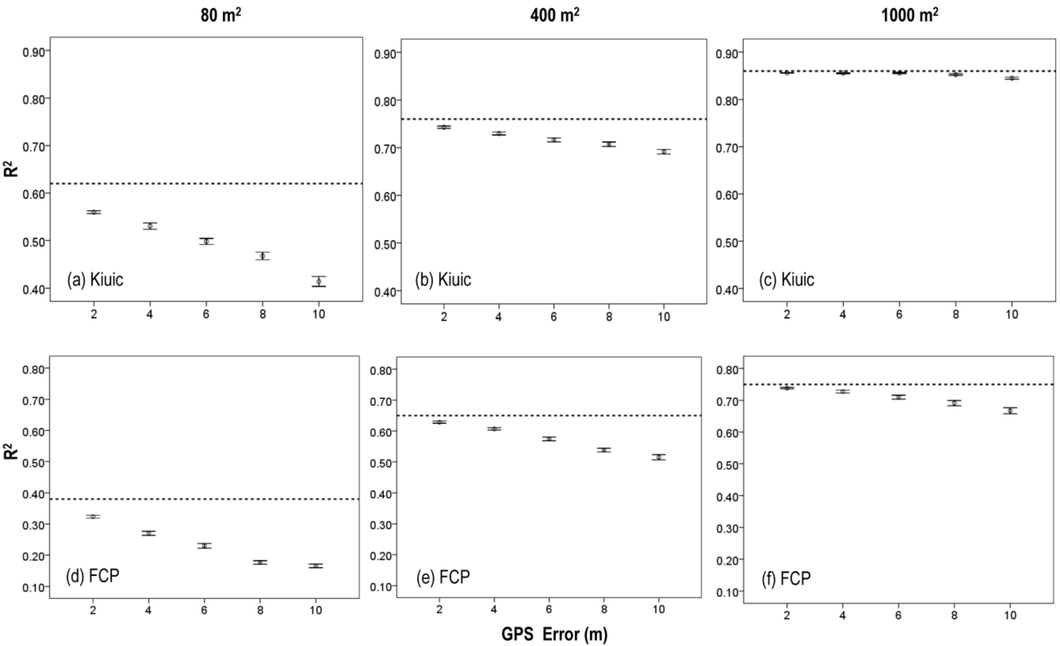
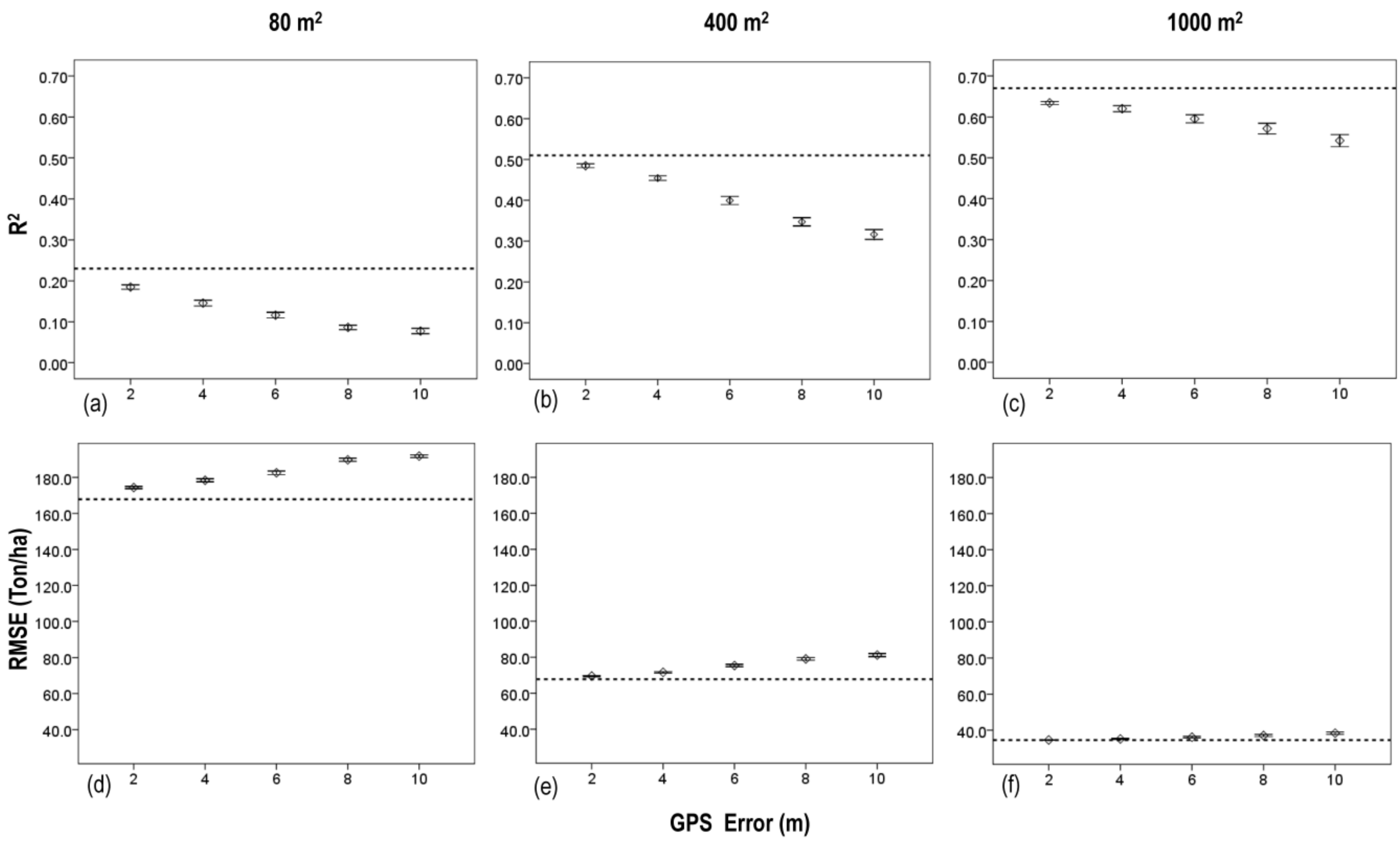
3.3. Effects of Plot Position Error and Plot Size

As the GPS location errors increased, the goodness of fit statistics (R2) obtained in the regression models for both sites decreased. For example, considering the 80 m2 plot in Kiuic (see Figure 3a), the mean R2 values decreases from 0.56 to 0.41 with GPS location errors of 2 to 10 m. However, when we compared the location error among sample plot sizes, the differences between the R2 value of the regression models using the differential GPS (dotted line in the graph) and the R2 values of the simulated GPS location errors decreased as plot size increased. For instance, in the 1000 m2 plot for Kiuic (see Figure 3c), the R2 value of the regression models with GPS location errors from 2 to 10 m (0.85–0.84) were very close to the R2 value with the differential GPS (0.86). When comparing both sites, the difference between the R2 values of the regression models with simulated GPS location errors and that of the differential GPS were smaller for Kiuic than for FCP.
The cross validations showed a similar pattern to the fitted regression models with R2 values decreasing as GPS location error increased. Conversely, mean values of RMSE increased with increasing GPS location error, both for Kiuic (Figure 4) and for FCP (Figure 5). For example, considering the 80 m2 plot in FCP (see Figure 5a), the mean R2 values decreases from 0.19 to 0.08 and RMSE increased from 174.3 to 191.8 Mg ha−1 as GPS location error increased from 2 to 10 m. When comparing GPS location errors among sample plot sizes, the R2 and RMSE values showed smaller differences between the different simulated location errors and the location with the differential GPS (dotted lines in Figure 4 and Figure 5) for the largest plot size (1000 m2), compared to the smallest size (80 m2). This means that the effect of GPS location error is substantially smaller in larger plots. When comparing both sites, the differences between R2 and RSME values of the procedures calculated for different GPS location errors and with the differential GPS were smaller for Kiuic than for FCP, indicating a smaller effect of location error and more robust models for Kiuic than for FCP.
The effect of GPS location error is largely driven by the overlap between field plot and LiDAR data. Thus, as the percent overlap decreases, the mean differences between RMSE of altered positions and the RMSE calculated with the differential GPS also increase in both sites (Figure 6). Moreover, the effect of plot size is much smaller when the percent overlap is considered. For example, for a comparable percent overlap (60 to 66%), the differences of RMSE between simulations and differential GPS locations are only 2.5 to 6.6 Ton/ha in Kiuic, and 4.4 to 8 Ton/ha in FCP. However, there is still a clear effect of plot size even when comparing a similar percent overlap, with larger plots showing consistently smaller errors in both sites. Finally, the FCP site showed larger differences between simulated and differential GPS location errors compared to Kiuic (Figure 6).

4. Discussion

Our results clearly show that sample plot size strongly influences the precision of AGB estimations from LiDAR data as well as the effect of plot location error, and that the precision of estimations and the effects of plot size and plot location error vary with tropical dry forest type. In agreement with our first prediction, the models for estimating AGB and the cross validation results both indicate that the accuracy of AGB estimates obtained from LiDAR increased with sample plot size (from 80 m2 to 1000 m2) in both types tropical dry forest investigated. The validation results showed an increase in the R2 values from 0.33 to 0.75 in the semi-deciduous forest (Kiuic) and from 0.23 to 0.67 in the semi-evergreen forest (FCP), as well as a concomitant decrease in the RMSE values from 103.26 to 27.98 Mg ha1 in Kiuic and from 167.85 to 34.47 Mg ha−1 in FCP as a plot size increased from 80 m2 to 1000 m2. These findings concur with previous studies in both temperate [20,21,38] and tropical forests [39,40] highlighting the importance of selecting an appropriate plot size for forest inventories used for estimating forest biomass. Studies in tropical dry forests in Malawi using photogrammetric data showed the same trend of increasing accuracy with increasing sample plot size [41].
The effect of sample plot size on the accuracy of AGB estimates from LiDAR data can be attributed to three main factors. First, relatively large areas must be sampled to accurately capture the patchy spatial distribution of small- and especially large-sized trees. Small plots often fail to capture the spatial heterogeneity of tree distribution, resulting in either over estimation—when a plot falls in an area containing a few large tress and/or large clumps of small trees—or underestimations —when the plot falls in an area lacking both large trees and large clumps of small trees [22]. Second, a larger sampled area samples a greater variation in population and community attributes (such as AGB), thereby providing a more accurate representation of the mean values of such attributes, hence more accurate estimates, compared to a smaller sampled area. Third, the perimeter-to-area ratio decreases with plot size, thereby reducing edge effects on AGB estimations from LiDAR. These effects result from a mismatch between field measurements of AGB, which are based on tree stems that fall within the plot area, and LiDAR metrics, which encompass all woody and foliar material within the plot area. Thus, the cloud of LiDAR points generally includes parts of crowns of trees whose stems fall outside the limits of the plot (and are therefore not included in field-based measures of AGB), and also excludes parts of the crowns of trees that are outside the plot area, although the stems are inside (and are therefore included in field-based measures of AGB). Since a circle is the geometric 2-D figure with the lowest perimeter-to-area ratio [39], the use of large circular plots, as in this study, minimizes edge effects [42], thereby improving the accuracy of AGB estimates from the LiDAR data.
Interestingly, although the accuracy of AGB estimates increased with increasing plot size, the marginal increase in accuracy declined as plot area increased. Thus, the R2 values of cross validations increased by 0.25 (a 76% increase) from 80 m2 (0.33) to 400 m2 (0.58) but only by 0.17 (a 29% increase) from 400 m2 to 1000 m2 (0.75) in Kiuic, and by 0.28 (a 120% increase) from 80 m2 (0.23) to 400 m2 (0.51) but only by 0.16 (a 31% increase) from 400 m2 to 1000 m2 (0.67) in FCP. These results are relevant because, as plot sizes increases, the cost of field sampling also increases [41]. Therefore, the selection of an optimal plot size for AGB estimation from LiDAR data should take into account a trade-off between estimation accuracy and plot establishment cost. Based on simulations using only LiDAR data, Frazer et al. [21] found an asymptotic non-linear relationship of the accuracy of AGB estimations with sample plot size and negligible increases in estimation accuracy for plots larger than 1257 m2. In our study, LiDAR estimations were based on field measurements of AGB for three sample plot sizes, and we found R2 values for the largest plot area that are comparable to those of Frazer et al. [21] and Mauya et al. [39], suggesting that it may not be necessary to increase the plot area much beyond 1000 m2, since this area provides reliable estimates of AGB, especially for the semi-deciduous tropical dry forest.
Another important finding of this study was that AGB estimations from LiDAR data are affected by GPS location errors, and that the effect of these errors decreases with increasing sample plot size and increasing overlap area between field and LiDAR data, supporting our second prediction. The R2 values consistently decreased as the location error increased for all three plot sizes in both forest types (Figure 3). Conversely, across sample plot sizes and in both forest types, the RMSE values of the cross validations increased as GPS location errors also increased (Figure 4 and Figure 5). Similar results have been reported by Zhang et al. [43] using Landsat TM data and by Frazer et al. [21] using LiDAR data. However, large plots were less affected by co-registration error compared to small plots. This is partly because an increase in plot size allows more overlap between ground plot and LiDAR data (see values of X axes in Figure 6), thereby reducing the potential errors associated with inaccurate GPS locations [21,44]. This is another reason why selecting the appropriate plot size for forest field inventories is of paramount importance to accurately estimate forest biomass from remote sensing data. Although there are alternative approaches trying to link field-surveyed tree locations with positions of trees identified by LiDAR and using an automatic procedure in order to reduce co-registration errors [23,45,46], the use of large plots has the advantage of capturing an adequate amount of structural variability in the field [22], reducing edge effects and increasing overlap area [41].
Finally, we found that the effects of sample plot size and GPS location error on estimations of AGB from LiDAR data varied between the two main types of tropical dry forest in the Yucatan Peninsula. In agreement with our third prediction, the accuracy of AGB estimates from LiDAR was higher, whereas the effects of sample plot size and plot location errors were smaller in Kiuic (semi-deciduous forest) compared to FCP (semi-evergreen forest). The smaller effect of plot size in Kiuic can be gauged from a lower percent increase in the accuracy of AGB estimates from the 80 m2 plot size to the 1000 m2 size in Kiuic (127%), compared to FCP (191%). The effect of plot location error showed a similar pattern, with smaller reductions in the mean R2 values and increases in RMSE values, as well as smaller differences in RMSE between simulated and differential GPS positions in Kiuic, compared to FCP (Figure 4, Figure 5 and Figure 6). Considering that we used the same LiDAR sensor and flight conditions in both sites, and that we applied local allometric equations for each site, the differences in model performance between forest types are likely attributable mostly to differences in vegetation density and forest structure complexity. The semi-deciduous tropical dry forest of Kiuic has a less complex vegetation structure compared with that of FCP, a semi-evergreen tropical dry forest [26]. As the complexity of vegetation structure increases, the probability that laser pulses penetrate the canopy decreases. Therefore, the point density below the canopy may be reduced, which may affect the values of LiDAR metrics [47], thereby reducing the accuracy of AGB estimations. In a meta-analysis, Zolkos et al. [23] found significant differences in AGB estimations from remote sensing data among different vegetation types. Moreover, the relationships between AGB field measurements and LiDAR data are also reported to vary with disturbance and along forest succession [20,48]. These combined results indicate that different vegetation types should be considered separately and that disturbance and forest successional age should be taken into account to accurately estimate and map forest AGB from LiDAR and other remote sensors.

5. Conclusions

In this study we evaluated the impacts of sample plot size and plot location errors on the accuracy of AGB estimations predicted from LiDAR data for two different tropical dry forests. Our results show that the accuracy of AGB estimations from LiDAR increases as plot size increases; decreases with increasing simulated plot location error, and that the effect of location error decreases as plot size increases. These results highlight the importance of sample plot size for AGB estimations from forest inventories using LiDAR and that plot size has a positive influence on the accuracy of AGB estimates. However, the selection of an optimal plot size should consider a trade-off between minimizing estimation errors and minimizing plot establishment costs. Our results suggest that, for the seasonally dry tropical forests studied, a plot size of 1000 m2 can provide accurate estimates of AGB that are robust to plot location errors of up to 10 m. Finally, the accuracy of AGB estimation from LiDAR data was higher and the effects of sample plot size and plot location errors were smaller in the structurally less complex semi-deciduous tropical dry forest of Kiuic, compared to the more complex semi-evergreen forest of FCP. Therefore, different vegetation types should be considered separately to accurately estimate and map forest AGB from LiDAR and other remote sensors at the landscape and regional levels.

Author Contributions

J.L.H.-S. conceived the research and designed the experiments. G.R.-P. and J.L.H.-S. analyzed the data. J.L.H.-S. and J.M.D. wrote the paper. All authors collected and processed field data, discussed the results, commented on the manuscript and shared equally in the editing of the manuscript.

Funding

The study was financially supported by Ecometrica LTD and the United Kingdom Space Agency in the framework of the project Forest 2020. The differential GPS equipment used in this study was acquired through the project “Medición a largo plazo de carbono y agua en una selva seca de Yucatán”, funded by the Mexican National Council of Science and Technology (CONACyT)—INFR 2016 01-269841.

Acknowledgments

We warmly thank the people from the “ejidos” of Xkobenhaltun and San Agustín in Yucatan and U’yoolché in Felipe Carrillo Puerto, Quintana Roo, for their permission to work on their land and assistance during fieldwork. Kaxil Kiuic A.C. provided logistic support. We also, want to thank Filogonio May-Pat for his help with fieldwork and species identification.

Conflicts of Interest

The authors have declared that no competing interests exist.

References

  1. Thomson, A.; Calvin, K.; Chini, L.; Hurtt, G.; Edmonds, J.; Ben Bond-Lamberty, B.; Frolking, S.; Wise, M.A.; Janetos, A.C. Climate mitigation and the future of tropical landscapes. Proc. Natl. Acad. Sci. USA. 2010, 107, 19633–19638. [Google Scholar] [CrossRef] [PubMed] [Green Version]
  2. Portillo-Quintero, C.A.; Sánchez-Azofeifa, G.A. Extent and conservation of tropical dry forests in the Americas. Biol. Conserv. 2010, 143, 144–155. [Google Scholar] [CrossRef]
  3. Le Quéré, C.; Peters, G.P.; Andres, R.J.; Andrew, R.M.; Boden, T.; Ciais, P.; Friedlingstein, P.; Houghton, R.A.; Marland, G.; Moriarty, R.; et al. Global carbon budget 2013. Earth Syst. Sci. Data Discuss. 2013, 6, 689–760. [Google Scholar] [CrossRef]
  4. Miles, L.; Newton, A.; Defries, R.; Ravilious, C.; May, I.; Blyth, S.; Kapos, V.; Gordon, J. A global overview of the conservation status of tropical dry forests. J. Biogeogr. 2006, 33, 491–505. [Google Scholar] [CrossRef]
  5. Sanchez-Azofeifa, G.A.; Castro-Esau, K.L.; Kurz, W.A.; Joyce, A. Monitoring carbon stocks in the tropics and the remote sensing operational limitations: From local to regional projects. Ecol. Appl. 2009, 19, 480–494. [Google Scholar] [CrossRef] [PubMed]
  6. Foody, G.M.; Boyd, D.S.; Cutler, M.E.J. Predictive relations of tropical forest biomass from Landsat TM data and their transferability between regions. Remote Sens. Environ. 2003, 85, 463–474. [Google Scholar] [CrossRef]
  7. Lu, D.; Chen, Q.; Wang, G.; Moran, E.; Batistella, M.; Zhang, M.; Vaglio Laurin, G.; Saah, D. Aboveground forest biomass estimation with Landsat and LiDAR data and uncertainty analysis of the estimates. Int. J. For. Res. 2012, 2012, 1–16. [Google Scholar] [CrossRef]
  8. Carreiras, J.M.B.; Vasconcelos, M.J.; Lucas, R.M. Understanding the relationship between aboveground biomass and ALOS PALSAR data in the forests of Guinea-Bissau (West Africa). Remote Sens. Environ. 2012, 121, 426–442. [Google Scholar] [CrossRef]
  9. Sinha, S.; Jeganathan, C.; Sharma, L.K.; Nathawat, M.S. A review of radar remote sensing for biomass estimation. Int. J. Environ. Sci. Technol. 2015, 12, 1779–1792. [Google Scholar] [CrossRef] [Green Version]
  10. Dubayah, R.O.; Sheldon, S.L.; Clark, D.B.; Hofton, M.A.; Blair, J.B.; Hurtt, G.C.; Chazdon, R.L. Estimation of tropical forest height and biomass dynamics using LIDAR remote sensing at La Selva, Costa Rica. J. Geophys. Res. Biogeosci. 2010, 115, 1–17. [Google Scholar] [CrossRef]
  11. Næsset, E.; Okland, T. Estimating tree height and tree crown properties using airborne scanning laser in a boreal nature reserve. Remote Sens. Environ. 2002, 79, 105–115. [Google Scholar] [CrossRef]
  12. Drake, J.B.; Knox, R.G.; Dubayah, R.O.; Clark, D.B.; Condit, R.; Blair, J.B.; Hofton, M. Above-ground biomass estimation in closed canopy Neotropical forests using Lidar remote sensing: Factors affecting the generality of relationships. Glob. Ecol. Biogeogr. 2003, 12, 147–159. [Google Scholar] [CrossRef]
  13. Lefsky, M.A.; Cohen, W.B.; Spies, R.A. An evaluation of alternate remote sensing products for forest inventory, monitoring, and mapping of Douglas-fir forests in western Oregon. Can. J. For. Res. 2001, 31, 78–87. [Google Scholar] [CrossRef]
  14. Lefsky, M.A.; Harding, D.J.; Keller, M.; Cohen, W.B.; Caraba-jal, C.C.; Espirito-Santo, F.D.; Hunter, M.O.; de Oliveira, R. Estimates of forest canopy height and above-ground biomass using ICESat. Geophys. Res. Lett. 2005, 32, 1–4. [Google Scholar] [CrossRef]
  15. Asner, G.P.; Hughes, R.F.; Varga, T.A.; Knapp, D.E.; Kennedy-Bowdoin, T. Environmental and Biotic Controls over Aboveground Biomass throughout a Tropical Rain Forest. Ecosystems 2009, 12, 261–278. [Google Scholar] [CrossRef]
  16. Vincent, G.; Sabatier, D.; Blanc, L.; Chave, J.; Weissenbacher, E.; Pélissier, R.; Fonty, E.; Molino, E.F.; Couteron, P. Accuracy of small footprint airborne LIDAR in its predictions of tropical moist forest stand structure. Remote Sens. Environ. 2012, 125, 23–33. [Google Scholar] [CrossRef]
  17. Hernández-Stefanoni, J.L.; Dupuy, J.M.; Jhonson, K.J.; Birdsey, R.; Tun-Dzul, F.; Peduzzi, A.; Camal-Sosa, J.P.; Sánchez-Santos, G.; López-Merlín, D. Improving Species Diversity and Biomass Estimates of Tropical Dry Forest Using Airbone LiDAR. Remote Sens. 2014, 6, 4741–4763. [Google Scholar] [CrossRef]
  18. Goldbergs, G.; Levick, S.R.; Lawes, M.; Edwards, A. Hierarchical integration of individual tree and area-based approaches for savanna biomass uncertainty estimation from airborne LiDAR. Remote Sens. Environ. 2018, 205, 141–150. [Google Scholar] [CrossRef]
  19. Wing, M.G.; Frank, J. An examination of five identical mapping-grade global positioning system receivers in two forest settings. West. J. Appl. For. 2011, 26, 119–125. [Google Scholar]
  20. Gobakken, T.; Næsset, E. Assessing effects of positioning errors and sample plot size on biophysical stand properties derived from airborne laser scanner data. Can. J. For. Res. 2009, 39, 1036–1052. [Google Scholar] [CrossRef]
  21. Frazer, G.W.; Magnussen, S.; Wulder, M.A.; Niemann, K.O. Simulated impact of sample plot size and co-registration error on the accuracy and uncertainty of LiDAR-derived estimates of forest stand biomass. Remote Sens. Environ. 2011, 115, 636–649. [Google Scholar] [CrossRef]
  22. Chave, J.; Condit, R.; Aguilar, S.; Hernandez, A.; Lao, S.; Perez, R. Error propagation and scaling for tropical forest biomass estimates. Phil. Trans. R. Soc. B. 2004, 359, 409–420. [Google Scholar] [CrossRef] [PubMed]
  23. Zolkos, S.G.; Goetz, S.J.; Dubayah, R. A meta-analysis of terrestrial aboveground biomass estimation using lidar remote sensing. Remote Sens. Environ. 2012, 128, 289–298. [Google Scholar] [CrossRef]
  24. Brubaker, K.M.; Johnson, S.E.; Brinks, J.; Leites, L.P. Estimating canopy height of deciduous forests at a regional scale with leaf-off, low point density LIDAR. Can. J. Remote Sens. 2014, 40, 123–134. [Google Scholar]
  25. Hall, S.A.; Burke, I.C.; Box, D.O.; Kaufmann, M.R.; Stoker, J.M. Estimating stand structure using discrete-return lidar: An example from low density, fire prone ponderosa pine forests. For. Ecol. Manag. 2005, 208, 189–209. [Google Scholar] [CrossRef]
  26. Carnevali, G.; Ramírez, I.M.; González-Iturbe, J.A. Flora y vegetación de la Península de Yucatán. In Naturaleza y Sociedad en el Área Maya; Colunga GarcíaMarín, P., Larqué-Saavedra, A., Eds.; Academia Mexicana de Ciencias, Centro de Investigación Científica de Yucatán: Mérida Yucatán, México, 2003; pp. 53–68. [Google Scholar]
  27. Chave, J.; Andalo, C.; Brown, C.S.; Cairns, M.A.; Chambers, J.Q.; Eamus, D.; Lescure, J.P. Tree allometry and improved estimation of carbon stocks and balance in tropical forests. Oecologia 2005, 145, 87–99. [Google Scholar] [CrossRef] [PubMed]
  28. Ramírez, G.R.; Dupuy, J.M.; Ramírez, L.; Sánchez, F.J.S. Evaluación de ecuaciones alométricas de biomasa epigea en una selva mediana subcaducifolia de Yucatán. Madera y Bosques 2017, 23, 163–179. [Google Scholar] [CrossRef]
  29. Guyot, J. Estimation du Stock de Carbone dans la Végétation des Zones Humides de la Péninsule du Yucatan. Memoire de fin D’etudes. Bachelor’s Thesis, AgroParis Tech-El Colegio de la Frontera Sur, Chetumal Quintana Roo, México, 2011. [Google Scholar]
  30. Schnitzer, S.A.; DeWalt, S.J.; Chave, J. Censusing and measuring lianas: A quantitative comparison of the common methods. Biotropica 2006, 38, 581–591. [Google Scholar] [CrossRef]
  31. Frangi, J.L.; Lugo, A.E. Ecosystem dynamics of a sub-tropical floodplain forest. Ecol. Monogr. 1985, 55, 351–369. [Google Scholar] [CrossRef]
  32. CartoData. Available online: http://www.cartodata.com// (accessed on 28 August 2018).
  33. McGaughey, R.J. FUSION/LDV: Software for LIDAR Data Analysis and Visualization; United States Department of Agriculture, Forest Service, Pacific Northwest Research Station: Portland, OR, USA, 2012; p. 154. Available online: http://forsys.cfr.washington.edu/fusion/fusion_overview.html (accessed on 28 August 2018).
  34. R Development Core Team. A Language and Environment for Statistical Computing; R Foundation for Statistical Computing: Vienna, Austria, 2012; ISBN 3-900051-07-0. [Google Scholar]
  35. Zar, J.H. Biostatistical Analysis; Prenctice Hall: Upper Saddle River, NJ, USA, 1999. [Google Scholar]
  36. Picard, R.R.; Cook, R.D. Cross-validation of regression models. J. Am. Stat. Assoc. 1984, 79, 575–583. [Google Scholar] [CrossRef]
  37. Miller, D.M. Reducing transformation bias in curve fitting. Am. Stat. 1984, 38, 124–126. [Google Scholar]
  38. Levick, S.R.; Hessenmöller, D.; Schulze, E.D. Scaling wood volume estimates from inventory plots to landscapes with airborne LiDAR in temperate deciduous forest. Carbon Balance Manag. 2016, 11, 7. [Google Scholar] [CrossRef] [PubMed]
  39. Mauya, E.; Hansen, E.; Gobakken, T.; Bollandsås, O.; Malimbwi, R.; Næsset, E. Effects of field plot size on prediction accuracy of aboveground biomass in airborne laser scanning-assisted inventories in tropical rainforests of Tanzania. Carbon Balance Manag. 2015, 10, 1–14. [Google Scholar] [CrossRef] [PubMed] [Green Version]
  40. Asner, G.P.; Mascaro, J. Mapping tropical forest carbon: Calibrating plot estimates to a simple LiDAR metric. Remote Sens. Environ. 2014, 140, 614–624. [Google Scholar] [CrossRef]
  41. Kachamba, D.J.; Ørka, H.O.; Næsset, E.; Eid, T.; Gobakken, T. Influence of plot size on efficiency of biomass estimates in inventories of dry tropical forests assisted by photogrammetric data from an unmanned aircraft system. Remote Sens. 2017, 9, 610. [Google Scholar] [CrossRef]
  42. Goetz, S.; Dubayah, R. Advances in remote sensing technology and implications for measuring and monitoring forest carbon stocks and change. Carbon Manag. 2011, 2, 231–244. [Google Scholar] [CrossRef] [Green Version]
  43. Zhang, M.; Lin, H.; Zeng, S.; Li, J.; Shi, J. Impacts of plot location errors on accuracy of mapping and scaling up aboveground forest carbon using sample plot and Landsat tm data. IEEE Geosci. Remote Sens. Lett. 2013, 10, 1483–1487. [Google Scholar] [CrossRef]
  44. Gonçalves, F.; Treuhaft, R.; Law, B.; Almeida, A.; Walker, W.; Baccini, A.; Graça, P. Estimating aboveground biomass in tropical forests: Field methods and error analysis for the calibration of remote sensing observations. Remote Sens. 2017, 9, 47. [Google Scholar] [CrossRef]
  45. Dorigo, W.; Hollaus, M.; Wagner, W.; Schadauer, K. An application-oriented automated approach for co-registration of forest inventory and airborne laser scanning data. Int. J. Remote Sens. 2010, 31, 1133–1153. [Google Scholar] [CrossRef]
  46. Pascual, C.; Martín-Fernández, S.; García-Montero, L.G.; García-Abril, A. Algorithm for improving the co-registration of LiDAR-derived digital canopy height models and field data. Agroforest. Syst. 2013, 87, 967–975. [Google Scholar] [CrossRef]
  47. Erdody, T.L.; Moskal, L.M. Fusion of LiDAR and imagery for estimating forest canopy fuels. Remote Sens. Environ. 2010, 114, 725–737. [Google Scholar] [CrossRef]
  48. Knapp, N.; Fischer, R.; Huth, A. Linking lidar and forest modeling to assess biomass estimation across scales and disturbance states. Remote Sens. Environ. 2018, 205, 199–209. [Google Scholar] [CrossRef]
Figure 1. Location of the study: Kiuic and Felipe Carrillo Puerto (FCP).
Remotesensing 10 01586 g001
Figure 2. Results of cross validation analyses used to compare the performance of observed and predicted values of above ground biomass in Kiuic (ac) and FCP (df). R2 is the determination coefficient and RMSE is the root mean square error, expressed in Mg ha−1. All linear regression models were significant with p < 0.01.
Remotesensing 10 01586 g002
Figure 3. Mean values and 95% confidence interval of goodness of fit statistic (R2) obtained from regression models in plots with altered positions (2, 4, 6, 8, 10 m) generated with a Monte Carlo simulation (500 repetitions) for different plot sizes (80, 400 and 1000 m2) in both Kiuic (ac) and FCP (df) sites. Dashed horizontal lines are the R2 values estimated with the differential GPS.
Remotesensing 10 01586 g003
Figure 4. Mean values and 95% confidence interval of R2 (ac) and RMSE (df) obtained from cross validation data with altered positions (2, 4, 6, 8, 10 m) generated with a Monte Carlo simulation (500 repetitions) for different plot sizes (80, 400 and 1000 m2) in Kiuic. Dashed horizontal lines are the R2 and RMSE values estimated with the differential GPS.
Remotesensing 10 01586 g004
Figure 5. Mean values and 95% confidence interval of R2 (ac) and RMSE (df) obtained from cross validation data with altered positions (2, 4, 6, 8, 10 m) generated with a Monte Carlo simulation (500 repetitions) for different plot sizes (80, 400 and 1000 m2) in FCP. Dashed horizontal lines are the R2 and RMSE values estimated with the differential GPS.
Remotesensing 10 01586 g005
Figure 6. Mean values and 95% confidence intervals of differences between RMSE of altered simulated positions (2, 4, 6, 8, 10 m) and RMSE values estimated with differential GPS against percent overlap between field plot and LiDAR data, for each plot size: 80 m2 (a), 400 m2 (b) and 1000 m2 (c) in both sites (Kiuic and FCP). The negative overlap values indicate the percent distance (d) between LiDAR and field data relative to plot radius (r) when there is no overlap (d > r)—see Methods.
Remotesensing 10 01586 g006
Table 1. Summary of above ground biomass statistics of field data by plot size in Kiuic and FCP.
SiteNumber of PlotsPlot Size (m2)Plot Radius (m)Biomass (Mg ha−1)
Mean (std Deviation)
Kiuic29805.04163.16 (127.16)
40011.28155.03 (84.46)
100017.84137.06 (61.58)
FCP28805.04397.21 (193.01)
40011.28301.21 (98.18)
100017.84232.45 (58.25)
Table 2. Candidate models to estimate above ground biomass from LiDAR metrics using different sample plot sizes in Kiuic and FCP. For a description of the LIDAR metrics see McGaughey [33].
SitePlot Size
(m2)
Number of
Predictors
Explanatory VariablesR2AIC
Kiuic801Elev P750.5275.0
2Elev P70 + All returns above mode0.6270.0
3 *Elev P70 + Elev SQRT mean SQ + All returns above mode0.7560.0
4001Percentage all returns above 4.000.7246.0
2Percentage all returns above 4.00 + Percentage first returns above mean0.7643.0
3 *Elev variance + Percentage all returns above 4.00 + Percentage first returns above mean0.8040.0
10001Percentage all returns above 4.000.8619.0
2 *Elev variance + Elev P950.8717.0
3 *Elev maximum + Elev variance + Elev P900.8914.0
FCP801Elev P700.1787.0
2Percentage all returns above 4.00 + First returns above mean0.3880.0
3 *Elev P40+ Elev P50 + Elev P600.4679.0
4001Elev P600.6038.6
2Elev mode + (All returns above mode)/(Total first returns) × 1000.6539.0
3 *Elev mode + Elev MAD median + Elev P010.7036.0
10001Elev CV0.755.9
2 *Elev L3 + Percentage first returns above mean0.791.7
3 *Elev L3 + Percentage first returns above mean + (All returns above mean)/(Total first returns) × 1000.84−3.0
AIC (Akaike Information criterion value) and R2 values are shown. Best models are indicated in bold; the section is based on lower AIC values and no multicolinearity. * means with multicollinearity.
Table 3. Regression parameters of best models used to estimate above ground biomass from LiDAR metrics using different plot sizes in Kiuic and FCP. For a description of the LIDAR metrics see McGaughey [33].
SitePlot Size (m2)Independent VariablesβStd ErrorR2
Kiuc80Intercept2.812.300.62
Elev P701.490.25
All returns above mode0.0040.001
400Intercept8.603.550.76
Percentage all returns above 4.000.250.03
Percentage first returns above mean−0.130.06
1000Intercept1.200.850.86
Percentage all returns above 4.000.190.02
FCP80Intercept12.434.750.38
Percentage all returns above 4.000.340.09
First returns above mean−0.030.01
400Intercept1.742.980.65
Elev mode1.050.17
(All returns above mode)/(Total first returns) × 1000.060.02
1000Intercept25.761.250.75
Elev CV−25.652.98
Dependent variable is SQRT of biomass, independent variables included in the model all had p < 0.01.

