Indirect Estimation of Structural Parameters in South African Forests Using MISR-HR and LiDAR Remote Sensing Data

Abstract

Forest structural data are essential for assessing biophysical processes and changes, and promoting sustainable forest management. For 18+ years, the Multi-Angle Imaging SpectroRadiometer (MISR) instrument has been observing the land surface reflectance anisotropy, which is known to be related to vegetation structure. This study sought to determine the performance of a new MISR-High Resolution (HR) dataset, recently produced at a full 275 m spatial resolution, and consisting of 36 Bidirectional Reflectance Factors (BRF) and 12 Rahman–Pinty–Verstraete (RPV) parameters, to estimate the mean tree height (H_mean) and canopy cover (CC) across structurally diverse, heterogeneous, and fragmented forest types in South Africa. Airborne LiDAR data were used to train and validate Random Forest models which were tested across various MISR-HR scenarios. The combination of MISR multi-angular and multispectral data was consistently effective in improving the estimation of structural parameters, and produced the lowest relative root mean square error (rRMSE) (33.14% and 38.58%), for H_mean and CC respectively. The combined RPV parameters for all four bands yielded the best results in comparison to the models of the RPV parameters separately: H_mean (R² = 0.71, rRMSE = 34.84%) and CC (R² = 0.60, rRMSE = 40.96%). However, the combined RPV parameters for all four bands in comparison to the MISR-HR BRF 36 band model it performed poorer (rRMSE of 5.1% and 6.2% higher for H_mean and CC, respectively). When considered separately, savanna forest type had greater improvement when adding multi-angular data, with the highest accuracies obtained for the H_mean parameter (R² of 0.67, rRMSE of 31.28%). The findings demonstrate the potential of the optical multi-spectral and multi-directional newly processed data (MISR-HR) for estimating forest structure across Southern African forest types.

1. Introduction

Forests provide a broad range of ecosystem services, e.g., carbon sequestration, water regulation, fuelwood and timber production [1,2]. Information on forest structure, such as canopy cover, tree height or canopy volume, is needed to support the sustainable management of these resources [3]. Despite the South African Government’s legal requirement of reporting on the state of national forests on a three-year basis [4], there are no regularly updated national forest maps or spatial datasets describing woody structural diversity, e.g., canopy cover, tree height. To date in South Africa, the only quantitative spatial data on forests are available in the form of occasional global products, such as the 1 km global tree height map [5], the 30 m global tree cover maps [6,7], or the 30 m Sub-Saharan African tree height map [8]. However, there is uncertainty regarding the accuracies of these products at regional scales, particularly in open forest ecosystems such as savannas, due to limited calibration outside boreal and tropical forest or for tree height below 5 m [8,9,10].

Remote sensing (RS) technologies produce valuable data for mapping forest structural parameters at a variety of spatial scales. They are particularly useful for providing dense and frequent coverage over large areas, which thus enables the monitoring of forest structural parameters cost-effectively [11,12]. A number of studies have explored the capabilities of RS data for retrieving structural information of plant canopies, including those derived from LiDAR [13,14], Synthetic Aperture Radar (SAR) [15,16,17], or optical sensors or a combination of these [18,19,20]. Research using optical data mostly exploits multispectral observations from nadir-pointing instruments and/or single view imagery [21,22]. However, most of the Earth’s continental surfaces, due to their three-dimensional characteristics, are strongly anisotropic, i.e., for a given illumination (sun) angle the reflectance changes with the viewing direction [23,24]. As a consequence, vegetation structural and biochemical variables largely control the surface reflectance anisotropy [23,25,26,27,28], which is described by the bidirectional reflectance distribution function (BRDF) [29]. The BRDF of a surface target is a function describing the ratio of the spectral radiance reflected in a given direction to the irradiance received by this target according to a specific illumination geometry; hence it measures reflectance changes with the illumination and observation geometry [23]. In practice it is not possible to measure the BRDF directly, and it is estimated by the bi-directional reflectance factor (BRF) [30,31]. Reflectance anisotropy has often been ignored or considered to be a source of noise for mapping forests [32,33].

Mono-angular, generally nadir-pointing, instruments can collect multi-angular data by accumulating data over repeated overflights or orbits (e.g., 16 days in the case of MODIS) [34,35]. However, this approach is inherently hindered by the daily evolution of the surface as well as atmospheric changes [35]. Optical multi-spectral and multi-directional (MSMD) instruments may offer promising opportunities [34,36,37,38]. MSMD instruments acquire quasi-simultaneous surface reflectance measurements in multiple spectral bands at various observation angles [39]. Examples include the POLarization and Directionality of the Earth’s Reflectance’s (POLDER) instrument or the Multi-Angle Imaging SpectroRadiometer (MISR) [28]. The MISR instrument is hosted on the NASA’s Earth Observation System (EOS) Terra platform, launched on 18 December 1999 [37]. At present, MISR is the only multi-angular earth observation satellite instrument sampling the anisotropy of the reflected solar radiation at sub-km spatial resolution. It uses nine cameras pointing at various angles fore and aft of the platform, each acquiring data in four spectral bands: three in the visible and one in the near-infrared range [26]. For any given location, all multi-directional data channels are acquired within less than seven minutes [40,41].

Studies based on MISR data have shown that using multi-angular observations improves the estimation of canopy structural parameters [40,42,43]. For instance, Heiskanen [44] reported that tree cover and height could be retrieved more effectively from MISR surface BRF data in Finland’s Fennoscandia tundra–taiga transition zone. At the 1.1 km spatial resolution, the relative root mean square error (rRMSE) for tree height and tree cover were 35.4% and 49.2% when using the spectral bands from the nadir camera only, and dropped to 25.4% and 36.9%, respectively, when using the spectral bands from all 9 cameras. Further, theoretical and applied studies have established that synthetic parameters describing reflectance anisotropy of land surfaces can also be used successfully to characterise the structural properties of vegetation [41,42,45]. One such model is the Rahman-Pinty-Verstraete (RPV) model, which describes the BRF of a surface using a combination of three parameters ρ₀, k, and $\Theta$ [41,45,46,47]. The ρ₀ parameter is a measure of the mean spectral brightness of the target [26,48,49,50]. The k parameter controls whether the reflectance anisotropy exhibits the usual bowl-shaped (k < 1), or a bell-shaped (k > 1) pattern, which has been associated with heterogeneous canopy conditions [41,47] and the $\Theta$ parameter captures the degree of forward or backward scattering [51]. Previous investigations suggested that multi-angular reflectance measurements may lead to an improved characterization and monitoring of vegetation structural properties [26,48,49,52].

The MISR instrument is designed to acquire observations with an across-track sampling distance of 250 m at nadir and 275 m in all off-nadir cameras. However, due to the downlink restriction only 12 of the 36 data channels are transmitted at full spatial resolution in the default Global Mode: The four spectral bands of the nadir camera and the red spectral band in each of the other eight cameras. The raw measurements in the remaining 24 data channels are spatially averaged on-board the platform to yield an effective 1.1 km pixel size. As a result, all MISR NASA-generated land surface products are delivered at this spatial resolution, and most MISR-based studies have relied on 1.1 km or coarser datasets. This is an important limitation in Southern Africa where forested landscapes are occupied by heterogeneous savannas dominated by a grass layer and variable (20–70%) woody cover, or consist of remnants of indigenous forests or stands of commercial plantation forests of variable but generally small stand sizes. At the landscape scale, structural patterns along catenae vary over distances between 100 and 300 m in savannas. Recently, however, the MISR High-Resolution (HR) processing system was developed to reconstruct the original spectral observations at their full spatial resolution (275 m) in all 36 data channels [53]. In addition, that system generates a suite of biogeophysical products—e.g., the RPV model parameters, the Leaf Area Index (LAI), or the Fraction of Absorbed Photosynthetically Active Radiation (FAPAR), among others—at that same resolution [53]. We hypothesized that the newly processed high resolution MISR MSMD data at 275 m spatial resolution across all the spectral bands should yield improved canopy structural parameter estimates, compared to traditional nadir-pointing instruments [37,38,44,54]. Pinty et al. [41] showed that the capacity to characterize the anisotropy degrades rapidly with the spatial resolution beyond 1km, where all surfaces appear to be the same “bowl-shape”. Hence, there is a great incentive in documenting the performance of anisotropic data at finer spatial resolution [26,41,55].

The aim of this study was to assess to what extent two of the MISR-HR 275 m data products, namely the 36 surface bidirectional reflectance factors (BRF) and the 12 RPV model parameters (ρ₀, k, Θ in each of the four spectral bands), may be used to estimate forest vegetation structural parameters (i.e., mean tree height and canopy cover) in South African forests, including savannas woodlands, indigenous dense forests, and commercial plantation forests. This study addressed three research questions:

• Do off-nadir MISR-HR products significantly improve the estimation of structural parameters compared to those obtained with the nadir-pointing camera only?
• Which data channels or combinations thereof, have the greatest potential to improve the canopy structure models performance?
• Does the performance of predicting structural parameters improve whilst using the MISR-HR RPV model parameters (ρ₀, k, Θ) compared to the full MISR-HR BRF multi-angle multi-spectral dataset (i.e., 4 spectral bands at nine view angles)?

These questions were answered using various scenarios based on MISR-HR data channel combinations elaborated in detail in Section 3.4. The inputs to our predictive models were the MISR reflectance data (BRF) and derived products (the RPV model parameters), which are the explanatory variables, generated by the MISR-HR processing system. High resolution airborne LiDAR data were used to derive the tree height and canopy cover products, which were used as reference data to train and validate the models.

2. Materials and Methods

This paper explores the strength of quantitative relationships between two forest structural parameters, tree height and canopy cover, derived from airborne LiDAR measurements at very high spatial resolution (1 m) and selected MISR-HR products, namely the surface BRF in 36 data channels and the 12 RPV data channels, for the two South African sites and for closely related acquisition dates. The two pre-processed spectro-directional MISR-HR products were converted and re-projected to TIFF WGS 84 images. A 275 m fixed grid snapped to the MISR pixels was used for extracting LiDAR-derived forest structural parameters, MISR-HR BRF reflectance, and RPV parameter values. The MISR-HR products were used as predictive (independent) variables with Random Forests (RF) algorithms (Breiman, 2001) (Figure 1) to retrieve the forest structural parameters according to a number of scenarios. The best model results were used to derive MISR-HR BRF-based maps of the structural parameters at 275 m spatial pixel size. The overview of the methodology is summarized and compiled in a flowchart (Figure 1).

2.1. South African Forested Landscapes and Study Area

The study area consists of two sites, (i) the South African Lowveld including the southern section of the Kruger National Park (KNP) and surrounding communal lands in the Mpumalanga and Limpopo Provinces and (ii) the iSimangaliso St-Lucia region in the KwaZulu-Natal Province. The sites were selected to capture the main forest types present in South Africa—including open forests such as savannas or woodlands, denser closed canopy indigenous forests of high biodiversity value, and commercial plantation forests.

The Lowveld site lies within the semi-arid savanna woodlands biome in the northeastern region of South Africa (Figure 2a). Savannas are characterised by a heterogeneous mixture of herbaceous and woody vegetation [56,57]. Rainfall is strongly seasonal, with a rainy summer season from October to May and a dry season from June to September. Rainfall occurs mostly in the form of thunderstorms with mean annual precipitation of 650 mm [58]. Mean annual temperatures reach 21 °C. These savannas are dominated by granitic woody landscapes of fine- and broad-leaf deciduous trees and grassy bushveld with a few scattered shrubs and trees in gabbro or basalt substrates [59,60]. The woody canopy cover ranges from wooded grassland (5%) to almost closed woodlands (60–70%), with tree height typically varying between 2 and 5 m. Woody Above Ground Biomass (AGB) is generally below 50 tons per hectare (T ha⁻¹). Land tenures include state-owned communal lands, privately-owned reserves (Sabie Sands Game Reserve) and state-owned conservation lands in the KNP (Figure 2a). Fuelwood harvesting and livestock ranching are predominant in communal savannas and woodlands.

The second site is located in the northeastern part of KwaZulu-Natal province of South Africa, in the iSimangaliso St-Lucia region (Figure 2b). Forested lands consist mostly of indigenous coastal forests (e.g., Dukuduku forest) and commercial forest plantations. This coastal area is characterized by all year round rainfall (with a seasonal minimum between June and September) reaching 1250 mm yr⁻¹, and a mean temperature of 27 °C [61,62]. South African indigenous forests are fragmented into small patches [61,63]. The Dukuduku coastal forest is the largest remaining indigenous coastal lowland forest patch (estimated around 3500 ha in area) [64]. It is surrounded by informal settlements, a matrix of sugarcane plantations, grassland as well as commercial Eucalyptus forest plantations. The coastal forest in this region is a subtropical moist evergreen broadleaf forest with medium to tall trees which can grow to about 20 m high [59,61]. The coastal forest region, in and around the Dukuduku forest, is species rich and with a well-developed closed canopy with fairly dense understory shrubs and a tree cover in excess of 70% [61]. The commercial forest plantations are mainly dominated by Eucalyptus spp. [65], with a height of up to 30 m [66]. The E. grandis stands have rotation lengths varying from 6–12 years and the AGB can be relatively high ranging between 106 and 225 (T ha⁻¹) [67,68]. In this manuscript, we refer to Lowveld and iSimangaliso Saint-Lucia for the two sites described above.

2.2. LiDAR Data

The forest structural parameters were derived from two discrete airborne LiDAR datasets. The first dataset consisted of approximately 63,000 ha of savannas surveyed over the Lowveld study area during April–May 2012 (Figure 2a), with the Carnegie Airborne Observatory-2 Airborne Taxonomic Mapping Systems (CAO-2 AToMS) [69]. The CAO-2 LiDAR scanner system (1064 nm) was operated in discrete mode at 1000 m above ground, with a laser pulse repetition frequency of 50 kHz, a laser spot spacing of 0.56 m, and yielded an average density of 6.4 points per m² [17,70]. The second dataset (29,000 ha) was acquired during April–May 2013 with a Leica ALS50 LiDAR, and a laser pulse repetition frequency of 150 kHz in the iSimangaliso St-Lucia site (Figure 2b). The dataset was made available by the iSimangaliso Wetland Park authority. The LiDAR point density was 1.5 points per m². Both datasets were collected at the wet to dry transition season. The senescence process was just starting in the Lowveld region, and most trees were still in leaf-on condition prior to winter and leaf shedding. Trees in the iSimangaliso St-Lucia landscape were also leaf-on as all species of the indigenous forests and plantations are evergreen.

2.3. LiDAR Processing and Derived Structural Parameters

The LiDAR-based forest structural parameters were derived from canopy height models (CHM) generated with a ground sampling distance of 1 m. The CHM was calculated by subtracting the Digital Elevation Model (DEM, last “ground” returns) from the Digital Surface Model (DSM, first “canopy” return), both derived from the raw LiDAR point clouds data as per the method outlined in [69]. A height threshold of 1 m was applied to all the CHM products, to exclude possible noise from non-woody vegetation (e.g., grass). The following structural metrics were calculated: Mean tree height (H_mean) and canopy cover (CC). The height threshold mentioned above implies that the structural metrics are calculated from the woody vegetation component including shrubs and trees, but we will refer to tree structural metric for simplicity. These structural parameters were computed as follows:

• Tree height is defined as the vertical distance from the base of the tree to its treetop [71]. It plays a key role in forest ecosystem studies, for instance for predicting species richness and species distribution models [72,73] or for assessing fire severity and modelling fire escape mechanisms [74,75]. It contributes to estimate variables such as canopy volume and biomass [76,77]. The mean tree height (H_mean) parameter was calculated as the average of the CHM pixels excluding the non-tree pixels (<1 m) within each MISR-HR 275 m pixel. This is a useful measure especially in even-aged forests. There was a strong relationship between tree height estimated by the CAO CHMs and field measurements (R² = 0.93, p-value < 0.001 and standard error of 0.73 m), as described in Wessels et al. [78].
• Canopy cover (CC) is defined as the percentage area of a MISR-HR 275 m pixel covered by the vertical projection of tree crowns. As a simple 2D structural measure, CC is a key descriptor of ecosystems and is useful for monitoring vegetation changes, for instance habitat connectivity and fragmentation [79,80,81]. This parameter was estimated by calculating the percentage of CHM pixels with a height above 1 m relative to the total number of LiDAR pixels included in a 275 m MISR pixel. A strong relationship between CAO LiDAR-derived CC and field measurements was previously demonstrated for the KNP dataset (R² = 0.79, Root Mean Square Error (RMSE) of 12.4%) [17].

2.4. MISR Data and Processing

The MSMD satellite data used in this study were acquired by the MISR instrument, which features nine cameras. One camera is pointing towards nadir (designated An at 0.1⁰ zenith angle), while the eight off-nadir cameras are pointing in the forward (f) and aft or backward (a) direction (designated Df: 70.3⁰, Cf: 60.2⁰, Bf: 45.7⁰, Af: 26.2⁰, Aa: 26.2⁰, Ba: 45.7⁰, Ca: 60.2⁰ and Da: 70.6⁰) [53]. Each MISR camera uses a push-broom sensor, with separate detectors for the four spectral bands: blue (446.4 nm), green (557.5 nm), red (671.7 nm) and near infrared (864.4 nm). The swath width is about 380 km wide. As part of the pre-processing to Level 1B2, the four spectral bands of each camera are radiometrically calibrated, geo-rectified and spatially co-registered [41,82]. A detailed description of the instrument and processing can be found in Diner et al. [82]. As hinted earlier, to keep the data rate within the downlink allocation, only 12 of the 36 MSMD data channels are transmitted at full spatial resolution in the Global Mode of operation, and hence, all standard products generated by NASA Langley Atmospheric Research Center are delivered at a spatial resolution of 1.1 km or coarser. Recently, a MISR-High Resolution (HR) processing system [53,83] was designed to reconstruct observations at the original spatial resolution of 275 m in all spectral bands and for all cameras. This system also produced a full range of higher level products at 275 m spatial resolution, including RPV model parameters, spectral and broadband albedos, as well as key vegetation products such as LAI and FAPAR [53,83].

The BRF and RPV products used in this study were generated with the MISR-HR processing system, version 1.04-5, hosted at the Global Change Institute of the University of the Witwatersrand in Johannesburg, South Africa [83]. The following data are used as inputs to generate the MISR-HR products [53]:

• The MISR L1B2 Terrain-projected Global Mode data, which contains top of atmosphere (TOA) radiance measurements, resampled at surface level and topographically corrected.
• The MISR L2 Terrain–projected bottom of atmosphere (BOA) bidirectional reflectance factors (BRFs), generated by NASA’s standard processing system at 1.1 km spatial resolution.
• Geometric Parameters Product (GPP).
• Ancillary Geographic Product (AGP), which are the reference datasets containing the full latitude/longitude information.

The first step in the MISR-HR processing routine consists of reconstructing radiance data at the nominal “Top of the Atmosphere (ToA)” (the L1B3 product) at the full spatial resolution in all 36 data channels. Those data are then converted to surface reflectance (BRF product) by isolating the surface from the atmospheric contribution to the measurements. This process also screens out cloud-covered areas. The MISR-HR 12 RPV model parameters (ρ₀, k, $\Theta$ for each spectral band) are the result of the third step in the MISR-HR processing system (http://www.misrhr.org/rpv) [53]. These parameters are retrieved by inverting the RPV model against the nine surface bidirectional reflectance values, separately in each of the four spectral bands. The bidirectional reflectance factor $\rho$ can be represented by the RPV model as follows [45,46]:

$$\rho \left({\theta }_s,\theta ,\varphi ,{\rho }_0,k,\Theta \right)={\rho }_{0}M\left({\theta }_s,\theta ,k\right)F_{HG}(g;{\Theta }_{HG})$$

(1)

where ${\theta }_S$, $\theta$ and $\varphi$ are the solar zenith angle, the observation zenith angle and the relative azimuth between the directions of illumination and observation, respectively, ${\rho }_0$ is the amplitude parameter of the RPV model and M is the modified Minnaert function.

$$M\left({\theta }_S,\theta ,k\right)=\frac{{\cos }^{k-1}{\theta }_S{\cos }^{k-1}\theta }{{\left(\cos {\theta }_S+\cos \theta \right)}^{1-k}}$$

(2)

M involves the power function of the zenith angle cosines governed by the $k$ parameter which describe the overall shape of the angular field, and

$$F_{HG}\left({\Theta }_{HG},g\right)=\frac{1-{{\Theta }^2}_{HG}}{{\left[1+2{\Theta }_{HG}\cos g+{{\Theta }^2}_{HG}\right]}^{3/2}}$$

(3)

$F_{HG}$ is the Henyey–Greenstein phase function, which uses the single parameter ${\Theta }_{HG}$ to characterize preferentially forward or backward scattering depending on its sign, and where

$$\cos g=\cos \theta \cos {\theta }_S+\sin \theta \sin {\theta }_S\cos \varphi$$

(4)

Detailed descriptions of the RPV model and its parameters are available in the literature [40,42,45,46,55]. The MISR-HR BRF and RPV products were converted from the native HDF-EOS format to GeoTIFF and re-projected from the original Space Oblique Mercator to UTM Zone (WGS 84 datum) projection to match the LiDAR CHM data.

Two MISR acquisitions were processed: The first one took place on the 10 April 2012 (Path 168, Orbit 65487, Block 110, covering the Lowveld site), and the second on the 6 April 2013 (Path 167, Orbit 70744, Block 113, covering the iSimangaliso St-Lucia site). These MISR acquisition dates were chosen primarily to correspond as closely as possible with the LiDAR data acquisition dates. In addition, images at the end of the wet season (autumn) have additional possible benefits. First, since grasses senesce earlier than trees, this period would produce a larger spectral contrast between dry grasses and green woody canopies, compared to images taken in the middle of the season when both grasses and woody canopies are green. Second, this period may also be more suitable than the summer, because the sun zenith angle is larger and this condition produces a wider range of projected shadows depending on vegetation structure and height, a condition which may enhance surface reflectance anisotropy.

2.5. Data Analysis

Canopy structural properties derived from LiDAR data (H_mean and CC), as well as MISR-HR BRFs and RPV products, were extracted using a regular 275 m spatial grid matching the MSIR-HR pixels. Only MISR pixels with full corresponding LiDAR coverage were considered. LiDAR and MISR-HR pixels which included 30% or more urban areas or cultivated fields were discarded using the 2013–2014 South African National Land-Cover (LC) map [84]. In addition, samples were filtered out when RPV values were retrieved with a high cost function value. The cost function value is the mathematical criterion that is minimized during the RPV model inversion procedure, and high values indicate poor data quality [53]. The differences in cost function values between the two sites most likely would result from varying environmental conditions which occurred during the two MISR orbits acquired one a year apart. Samples (i.e., MISR-HR data at pixel level) were removed from the two study sites when the cost value was larger than 40, across all the three RPV parameters and for all the bands. This threshold was selected through the assessment of the cost value histograms (Figure 3), considering published materials on the subject [85], and the necessary trade-off between a conservative threshold value for ensuring high RPV retrieval quality and maintaining a sufficient number of samples in the iSimangaliso Saint-Lucia site. The threshold used led to the removal of 131 pixels out of 6281 pixels for the Lowveld and 1000 pixels out of 2194 in iSimangaliso Saint-Lucia.

We used the non-parametric Breiman–Cutler Random Forest (RF) algorithm [86] to model the relationship between structural LiDAR data and MISR data. Parametric models (e.g., multi-linear regression models) lack the capability to adequately characterize forest complexity and suffer from various limitations, such as the assumption of linearity, sensitivity to overfitting, or multicollinearity [87,88]. Non-parametric models, Support Vector Machines [89], Artificial Neural Network [90] and Random Forest [91,92], have gained popularity due to their ability to model complex non-linear and multidimensional data [93,94]. RF is generally more robust to outliers and flexible in modelling relationships for large data sets with a large number of explanatory variables [91,95,96].

The Breiman–Cutler RF algorithm is built from bootstrap aggregation (bagging) and randomly selected subsets of explanatory variables, which create an ensemble classifier. RF regressions are easier to implement than optimally pruned decision trees, as they only require two user-defined inputs: ‘ntree’ which is the number of RF trees built in the forest and ‘mtry’ which is the number of possible splitting variables for each of the nodes [95,97]. The ‘mtry’ was set to the square root of the number of variables [98] (i.e., MISR predictor variables for a given scenario). The ‘ntree’ was optimized by testing decreasing numbers of trees in steps of 100, starting with the default value of 500, and assessing the minimum mean square error (MSE) [98,99]. This resulted in varying tree sizes per model, determined by the MSE. The models were implemented with the open source R software environment for statistical computing and graphics [100]. Training and test data were created via a 60/40% random split of the complete dataset and of the individual forest vegetation type.

The performance of the models was assessed using the coefficient of determination (R²), the root mean squared error (RMSE) (Equation (5)), the relative root mean square error (rRMSE) (Equation (6)), the bias (Bias) (Equation (7)), and the relative bias (rBias) (Equation (8)). RMSE and rRMSE were used as estimates of error or accuracy. The rRMSE and rBias were expressed in percentages in the Equations (6) and (8) respectively. The RMSE provides an estimate of modelling errors expressed in the original measurement units, and the rRMSE normalizes the RMSE according to the mean, allowing the comparison of models in which errors are measured in different units [101].

$$\mathrm{RMSE}=\sqrt{\frac{{{\displaystyle \sum }}_{i=1}^n{\left({\widehat{y}}_i-y_i\right)}^2}{n}}$$

(5)

$$\mathrm{rRMSE}=\frac{\mathrm{RMSE}}{\overline{y}}\times 100$$

(6)

$$\mathrm{Bias}=\frac{{{\displaystyle \sum }}_{i=1}^n\left({\widehat{y}}_i-y_i\right)}{n}$$

(7)

$$\mathrm{rBias}=\frac{\mathrm{Bias}}{\overline{y}}\times 100$$

(8)

where ${\widehat{y}}_i$ is the MISR estimated mean tree height or canopy cover, $y_{i }$ is the LiDAR measured mean tree height or canopy cover, $n$ is the number of observations and $\overline{y}$ is the mean LiDAR measured tree height or canopy cover. An analysis of variance (ANOVA) was used to test for any statistical significance between the models by comparing the critical F-value and the F-statistics. It was reported with the subscript of F as the first and second degrees of freedom which gave us the critical F value.

A number of scenarios were investigated to address the objectives of the study. The scenarios were based on different combinations of MISR-HR multi-spectral and multi-angular datasets, as well as the RPV anisotropic parameters. All the Lowveld samples were categorized as savanna vegetation. In the iSimangaliso St-Lucia site, the 2013–2014 Land Cover map mentioned in Section 3.4 was used to separate samples into indigenous forests and plantation forests. We analyzed the following scenarios:

• Scenario 0: The baseline reference scenario was set up to establish the expected performance of a RF model using a traditional approach based on the red and NIR spectral bands similar to that provided by the nadir-viewing instruments such as the MODIS instrument. These two MISR-HR datasets bands (at 275 m) have a similar pixel size to that of MODIS dataset (i.e., 250 m).
• Scenario 1: The first scenario considered all four spectral bands from the An (nadir) camera. This scenario was carried out to establish whether adding more spectral bands from the nadir-pointing cameras improves the predictive capacity of the RF model.
• Scenario 2: This second scenario sought to evaluate if angular data is superior to spectral data for the retrieval of the forest parameters, or vice versa. We developed a set of four models; each including all view angles for a single spectral band (i.e., one RF model for each of the MISR bands and involving all 9 cameras).
• Scenario 3: The third scenario assessed the RF model performance constrained by data in each view angle separately. It consisted of eight models including all spectral bands for each individual forward and aft viewing angle (i.e., off-nadir camera: Af, Bf, Cf, Df, Aa, Ba, Ca and Da).
• Scenario 4: The fourth scenario was carried out to ascertain whether the combined use of all MISR angular and spectral data (i.e., the 36 MISR-HR BRF data channels) improves the forest structural parameter retrievals compared to any of the previous scenarios and if it does by how much.
• Scenario 5: The fifth scenario assessed if the anisotropic BRF parameters provide additional benefits compared to the raw MISR-HR BRF data (scenario 4). Here, we tested four models, three models which assessed the performance of each individual RPV model parameter (ρ₀, k, Θ) considering all spectral bands, and one additional model combining all three RPV parameters for all spectral bands.

3. Results

This section documents the variability of the LiDAR-based structural parameters across the study sites (

Table 1. Descriptive statistics for the two LiDAR structural parameters, mean tree height (H_mean) and canopy cover (CC) per forest vegetation type, and for all the forest vegetation types together at 275 m spatial resolution.

	Lowveld-Savanna n = 6150		iSimangaliso St-Lucia Indigenous Forest n = 439		iSimangaliso St-Lucia Forest Plantation n = 755		Combined Samples n = 7344
Parameters	Hmean	CC	Hmean	CC	Hmean	CC	Hmean	CC
	(m)	(%)	(m)	(%)	(m)	(%)	(m)	(%)
Mean	3.6	24.3	6.19	48.9	11.7	50	4.6	29.6
SD	0.8	14.2	2.51	23.8	3.9	16.4	2.9	19.5
Min	1.2	0	1.02	0.9	1	1.6	1	0
Max	8.4	71.9	14.2	90.6	21.4	90.9	21.4	90.9
CV	0.2	0.6	0.4	0.5	0.3	0.3	0.6	0.7

), the performance of the retrieval of canopy structural parameters for all MISR-HR BRF and RPV model scenarios, for all vegetation types combined (

Table 2. Validation statistics of the predictive models for the mean tree height (H_mean) and canopy cover (CC) parameters at 275 m spatial resolution, using different spectral-angular combination of MISR BRF bands (all forest vegetation types or combined samples from Lowveld and iSimangaliso Saint-Lucia) (n = 7344).

Target Variable	Hmean (m)						CC (%)
View-Angle a (Spectral Bands b)	No. of Inputs	R2	RMSE (m)	rRMSE (%)	Bias	rBias (%)	No of Inputs	R2	RMSE (%)	rRMSE (%)	Bias	rBias (%)
Scenario 0 Nadir (red and NIR)	2	0.56	1.97	42.80	0.06	1.19	2	0.37	15.28	51.12	0.83	2.76
Scenario 1 Nadir(All)	4	0.66	1.73	37.36	0.07	1.43	4	0.51	13.36	44.69	0.21	0.71
Scenario 2 All(blue)	9	0.65	1.76	38.03	0.04	0.84	9	0.50	13.42	44.89	0.41	1.36
Scenario 2 All(green)	9	0.67	1.69	36.70	0.03	0.67	9	0.55	12.75	42.66	0.42	1.41
Scenario 2 All(red)	9	0.66	1.71	37.07	0.05	0.97	9	0.55	12.82	42.87	0.21	0.69
Scenario2 All(NIR)	9	0.66	1.72	37.27	0.02	0.39	9	0.54	13.16	44.22	0.32	1.06
Scenario 3 Off_Nadir_Df(All)	4	0.65	1.75	37.90	0.04	0.82	4	0.44	14.57	48.95	0.18	0.59
Scenario 3 Off_Nadir_Cf(All)	4	0.62	1.81	39.15	0.03	0.69	4	0.44	14.32	47.90	0.25	0.83
Scenario 3 Off_Nadir_Bf(All)	4	0.64	1.77	38.27	0.05	1.13	4	0.47	13.99	46.80	0.54	1.80
Scenario 3 Off_Nadir_Af(All)	4	0.66	1.72	37.29	0.06	1.30	4	0.49	13.58	45.43	0.32	1.07
Scenario 3 Off_Nadir_Aa(All)	4	0.66	1.73	37.44	0.04	0.87	4	0.49	13.59	45.45	0.45	1.50
Scenario 3 Off_Nadir_Ba(All)	4	0.66	1.74	37.68	0.02	0.35	4	0.47	13.88	46.43	0.47	1.56
Scenario 3 Off_Nadir_Ca(All)	4	0.66	1.75	37.83	0.04	0.93	4	0.49	13.89	46.67	0.04	0.14
Scenario 3 Off_Nadir_Da(All)	4	0.61	1.86	40.35	0.03	0.65	4	0.47	14.15	47.54	0.28	0.94
Scenario 4 All(All)	36	0.73	1.53	33.14	0.01	0.30	36	0.64	11.54	38.58	0.27	0.91

^a All = Df, Cf, Bf, An, Aa, Ba, Ca and Da cameras or view angles. ^b The color names ‘blue’, ‘green’, ‘red’ and ‘NIR’ refer to the corresponding spectral bands, All refers to all spectral bands. H_mean stands for Mean tree height and CC for canopy cover. The highest R² value for each scenario is shown in bold.

and

Table 3. Validation statistics of the predictive models for the mean tree height (H_mean) and canopy cover (CC) metrics at 275 m spatial resolution, using different parameters of the MISR RPV (all forest vegetation types or combined samples from Lowveld and iSimangaliso Saint-Lucia (n = 7344).

Target Variable	Hmean (m)						CC (%)
RPV Parameters a	No of Bands	R2	RMSE (m)	rRMSE (%)	Bias	rBias (%)	No of Bands	R2	RMSE (%)	rRMSE (%)	Bias	rBias (%)
Scenario 5 ρ0 (All)	4	0.65	1.76	38.22	0.00	0.00	4	0.49	13.90	46.69	−0.05	−0.15
Scenario 5 k (All)	4	0.62	1.83	39.59	0.01	0.24	4	0.48	13.94	46.84	0.00	0.01
Scenario 5 Θ (All)	4	0.48	2.14	46.32	−0.01	−0.11	4	0.43	14.71	49.42	0.14	0.47
Scenario 5All (All)	12	0.71	1.61	34.84	0.01	0.10	12	0.60	12.19	40.96	0.04	0.13

^aρ₀, = Rho parameter, k= the Minneart function, Θ = Theta parameter. All refers to all spectral bands. All also refers to all the RPV parameters (ρ₀, k, Θ). H_mean = Mean tree height and Canopy cover = CC. The highest R² value for the scenario is shown in bold.

, Figures 5–7), and for the scenarios 1 and 4, for the three vegetation types separately (savanna, indigenous forest and commercial forest plantations) (Figure 8).

3.1. LiDAR Based Strucutural Variability

The descriptive statistics (mean, standard deviation SD, minimum, maximum and coefficient of variation or CV) of the two LiDAR-derived parameters extracted at 275 m pixel size are shown in Table 1. The mean tree height (H_mean) followed an expected trend across the vegetation types with an increasing value from savannas (3.6 m) to indigenous forests (6.2 m), and then forest plantations (11.9 m). Savannas in the Lowveld are dominated by relatively small trees as indicated by the low H_mean CV (0.2) and with a range of mean tree height varying between 1.2 and 8.4 m. As expected, savanna was the most heterogeneous vegetation type with the lowest mean CC (22.3%) and the highest CC CV (0.6), while the maximum CC only reached 70%. The maximum H_mean was 14.2 m and 21.4 m for indigenous forests and forest plantations, respectively, in the iSimangaliso St-Lucia site. The mean CC for plantations and indigenous forests was higher than savannas at around 50% with a CV varying between 0.3 and 0.5. Plantations follow a typical growth cycle starting from bare ground up to a closed tall canopy, with height and cover varying significantly across stands of different ages. However, the CVs for both H_mean and CC in the indigenous forests were higher than expected (0.4 and 0.5, respectively), and were possibly due to two types of forest of different heights (i.e., Northern Coastal Forest and Mangrove Forest). Hence, the data exhibited a bimodal histogram, with two peaks for H_mean at the 4–5 m and 7–8 m and for CC at the 30–40% and 80–90% (Figure 4a,b). In addition, the wide range of H_mean and CC for indigenous forests may be exacerbated by bordering pixels in the Dukuduku forest fragmented landscape. The combined LiDAR datasets (all three vegetation types) cover a wide range of CC (0 to 90%) and height (1 to 21 m). However, the savanna samples largely dominate the dataset with 83.7% coverage, while indigenous and plantation forests make up 6.0% and 10.3% of samples, respectively.

3.2. Retriaval Performance from Nadir Reflectance

The Scenario 0 allows comparing a traditional approach using only the red and NIR spectral bands at 275 m spatial resolution at nadir (e.g., MODIS) with the Scenario 1, which includes two additional spectral bands (blue and green) at nadir. The results showed that for both H_mean and CC, the relative error value improved significantly when the number of bands was increased, with a decrease of 12.7% and 12.6% in rRMSE for H_mean and CC, respectively (Table 2). The performance improvement of Scenario 1 model was found to be statistically significant (F_{2, 7340} = 19.49, p < 0.05), for both parameters.

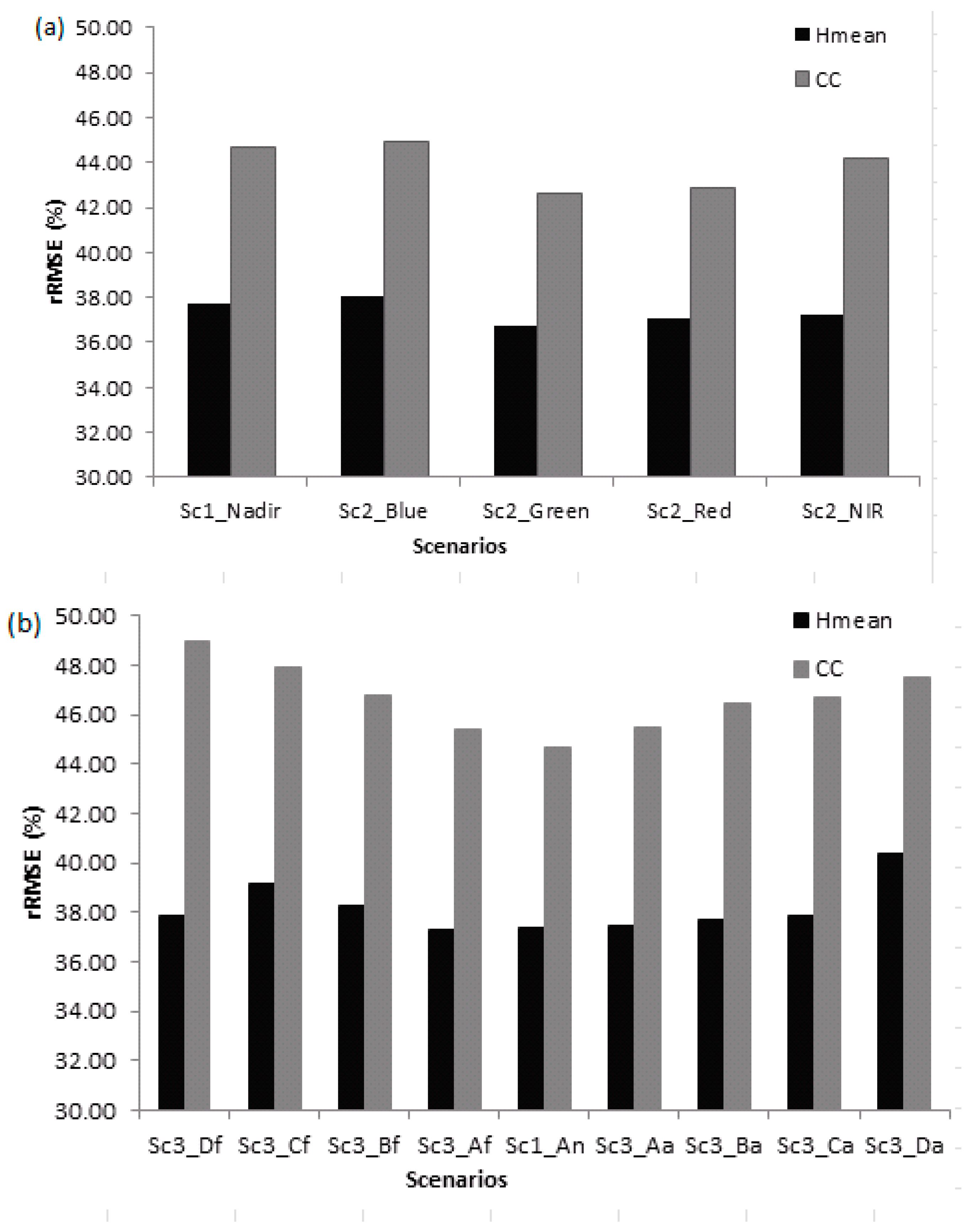
3.3. Comparison of Spectral Information Versus Angular Performance

The goal here was to establish whether spectral variability is more significant than angular variability for retrieving structural parameters, or vice versa. Thus, we compared Scenario 1—four spectral bands observed at nadir—against Scenario 2—single spectral band and multi-angular data (Table 2, Figure 5a). The Scenario 2 showed very similar performance when compared to the Scenario 1. The multi-angular green band model showed the smallest rRMSE, for both H_mean and CC, with a higher performance for H_mean (rRMSE = 36.7% versus 42.7% for H_mean and CC, respectively). However, this was only marginally lower than the model using all four spectral bands observed at nadir, with an improvement of 1.8% and 4.54% for H_mean and CC, respectively. The overall results indicated a minimal difference in model results when using multiple spectral bands observed at nadir versus multiple angular bands for a single spectral band. There was no statistical significant difference between Scenario 2 and Scenario 1 obtained for both the parameters (F_{5, 7335} = 4.36, p > 0.05).

3.4. Comparison of Single Angular MISR Cameras

Scenario 3 assessed the contribution of each off-nadir viewing angles individually (both forward and aft), including all four spectral bands, to determine their ability to predict the forest structural parameters and analyze off-nadir information content. The results showed that for both structural parameters the best angular configurations were either the nadir (An) or a small view angle close to nadir (Table 2, Figure 5b). Only a marginal difference in estimation error was observed for the H_mean parameter for the Af camera (rRMSE = 37.29%) compared to the An nadir camera of Scenario 1 (rRMSE = 37.36%). For the CC parameter, the An nadir camera produced a lower error than any of the off-nadir cameras. For both parameters, the model performance generally decreased as the view angle increased (further from the nadir) with no apparent difference for the fore and aft view angles (Scenario 3) (Figure 5b). The only statistically significant differences observed between Scenario 3 was between the Cf and Da cameras, (F_{1, 7340} = 254.30, p < 0.05) for both parameters.

3.5. Contribution of All 36 MISR Data Channels

The addition of all off-nadir bands to the nadir-only bands (Scenario 4, all 36 MISR data channels) showed a significant improvement of the predictive model performances compared to the nadir two spectral bands only (Scenario 0) or to the nadir four spectral bands (Scenario 1). Scenario 4 improved the relative rRMSE performance by 22% and 25% for H_mean and CC, respectively, compared to Scenario 0, and by 11.3% and 13.7% compared to Scenario 1 (Figure 6a). The highest coefficient of determination were also obtained for Scenario 4 with 0.73 and 0.64 for H_mean and CC, respectively (Table 2, Figure 5). This compared to the modest prediction improvement obtained between Scenario 1, and Scenario 2 suggests that the performance of multi-angle data is enhanced when using multispectral data. The model rBias decreased marginally for H_mean from 1.2–1.4 to 0.3% and from 2.8 to 0.9% for CC. While we obtained a lower rBias for H_mean, in the scatterplot of the validation model we still observed an overestimation of the prediction at the lower end of H_mean or CC, and an underestimation at the higher end (Figure 6b,c). The differences between the Scenario 0 and Scenario 4 models, and the Scenario 1 and Scenario 4, were both statistically significant and for both parameters (F_{34, 7308} = 1.63, p < 0.05; F_{32, 7308} = 1.63, p < 0.05).

3.6. Contribution of MISR-HR RPV Model Paramters

Scenario 5 evaluated the effectiveness of the RPV parameters in predicting the forest structural variables (Figure 7). We first assessed the RPV parameters (ρ₀, k, Θ) separately for all four spectral bands. The ρ₀, parameter produced the highest correlation and lowest estimation errors, with R² = 0.65, rRMSE = 38.22% and R² = 0.47, rRMSE = 46.69% for H_mean and CC, respectively (Figure 6a,b). The poorest performances were obtained for Θ with R² = 0.48, rRMSE = 46.32% and R² = 0.43, rRMSE = 49.42% for H_mean and CC, respectively. The best RPV model resulted from the combined use of all 12 MISR-HR RPV parameters for both H_mean and CC parameters, with rRMSE = 34.84% for H_mean and rRMSE = 40.96% for CC (Figure 7b). The 12 MISR-HR RPV parameter model did not perform as well (statistical significant p-value < 0.05) as the MISR-HR BRF 36 band model (Scenario 4) and produced a relative rRMSE of 5.1% and 6.2% higher for H_mean and CC, respectively. The H_mean and CC had similar trends and patterns across all scenarios with H_mean models generally performing better than CC models. Overall, for the combined forest type dataset the best model was obtained for the H_mean parameter using the 36 BRF data channel (R² = 0.73, rRMSE = 33.14%).

3.7. Model Performance across Vegetation Types

Overall, across all the vegetation types, there was a consistent model improvement with the addition of multiple off-nadir viewing angles in Scenario 4 compared to Scenario 1 (Figure 8). Nadir looking models in Scenario 1 produced consistently higher estimation errors and lower correlation for all the vegetation types individually. The benefits of the off-nadir viewing angles were higher for the savanna and indigenous forest models, where the estimation errors were consistently reduced by 25–35% for both parameters. The H_mean for savanna and CC for indigenous forest vegetation yielded the lowest estimation errors with rRMSE of 31.28% and 38.19%, respectively, and with the highest correlation R² of 0.67 and 0.57, respectively. The poorest performances were consistently obtained for the forest plantation models for both scenarios (e.g., highest rRMSE = 79% for Scenario 1) (Figure 8b).

4. Discussion

In this study, we investigated the use of MISR High-Resolution (HR) data products at 275 m spatial resolution—the 36 bi-directional reflectance factor data channels and 12 Rahman-Pinty-Verstraete model parameters (ρ₀, k, Θ in each of the 4 spectral bands)—to retrieve vegetation structural variables for different forest types, using Random Forest models. This section discussed several findings regarding the performance of multiple scenarios including the BRF multi-spectral nadir (Scenario 0 and 1), multi-angular and single spectral (Scenario 2), single off-nadir viewing angle (Scenario 3), combined multi-spectral and multi-angular (Scenario 4), as well as the RPV models (Scenario 5) based on the combined samples from the Lowveld and iSimangaliso St-Lucia sites. First, the RF model results based on the multi-spectral MISR-HR BRF measurements at nadir (Scenario 1 indicated considerable improvement over the traditional two bands approach (Red and NIR only, Scenario 0)) for both vegetation structural parameters. However, the multi-spectral nadir only (Scenario 1) compared to the single-spectral multi-angular model (Scenario 2) showed that equivalent results can be obtained with either spectral or directional data for both mean tree height and canopy cover. This finding was consistent with findings reported by other studies, that single band multi-angular information is not sufficient to estimate vegetation structural parameters [90,102,103].

The results obtained for the single off-nadir viewing angle and multi-spectral model (Scenario 3) for both vegetation structural parameters generally showed comparable results to the multi-spectral nadir only looking model (Scenario 1). We also observed that small off-nadir angles (i.e., Af) yielded lower errors than the off-nadir models with larger angles. This could be attributed to the fact that at nadir, or small off-nadir viewing angles, a greater proportion of gaps is visible which would result in increased reflectance as well as more structural information due to the higher visibility of the shading associated to woody components closer to the ground. Inversely, at larger viewing angles, the canopy gaps and shadows are less visible due to a change of perspective (side looking) and the canopy surface could be perceived as being smoother and more homogenous irrespective of height and cover [28,104]. The low accuracies obtained for both the single band multi-angle or single off-nadir multi-spectral models supported findings from other studies [90,103,105,106], that suggested that using only spectral or single angular information is less accurate in the estimation of vegetation structural parameters, this despite the retrieval of the MISR data at 275 m pixel size. On the one hand spectral reflectance data does not directly measure three-dimensional canopy structure hence it cannot provide explicit information on it [107,108], but rely on indirect effects such as shadowing. On the other hand single view data is limited in the estimation of vegetation structural data due to the forests’ three-dimensional characteristics (i.e., size, shape of canopies, position of trees) which result in varying reflection and distinctive pattern of shadows with varying view angles [23,25]. Various studies highlighted that single-view is not adequate in capturing forest structure as compared to multi-angular information [44,90,103].

The use of all the spectral and directional data (the 36 MISR data channels) in a single model yielded the highest estimates for both the mean tree height and canopy cover. This result was found to support several studies, which found improved retrieval of vegetation structural parameters when using multiple off-nadir angles with multi-spectral bands compared to using spectral data only at nadir [44,50,109].

This finding confirms the main hypothesis that increasing the number of off-nadir angular measurements from the newly processed high-resolution MISR MSMD data would yield improved canopy structural parameters estimates and lower estimation errors as compared to the nadir only measurements.

The MISR-HR BRF 36 data channels estimation model performance was slightly better, but comparable to the MISR-HR RPV all bands (12 bands) models for both forest structure parameters. The results showed a small rRMSE (1–2%) difference between these two models and differences were significant. In addition, the use of a non-parametric machine learning model such as Random Forest may have assisted to extract the non-linear anisotropic information present in the BRF data and synthesized by the RPV parameters. Hence the study supports the findings that RPV parameters contain vegetation structural information [26,48,55], which can be used in vegetation structural studies. These results could warrant making use of all the MISR-HR RPV all bands (12 bands) over MISR-HR BRF 36 data channels MISR-HR BRF 36 data channels which would mean data dimensionality reduction.

Each vegetation types had important difference in the heterogeneity of cover and height, which influenced the per vegetation type model results. The savanna (a spatially heterogeneous and open canopy environment) modelling results, were the best of all the three forest types, with the lowest estimation errors and highest coefficient of determination for H_mean, rRMSE = 32.28%, and R² value of 0.67 (Figure 8a,b). A possible explanation for the better model results in the savanna could be due to its open and heterogeneous canopy structure, resulting in shadows cast by the trees on the grassy background providing a stronger anisotropy signal. These conditions would not be prevalent at the opposite side of the woody canopy cover range, either at closed or no woody canopy cover. The indigenous forest exhibited fair results for the CC parameter which had the lowest estimation error (rRMSE = 38.19%) and an R² value of 0.57. However, the generated map (Figure 9) shown that it is difficult to obtain high accuracy in extracting height classes in these savanna environments in South Africa. The limited high precision in the derived map (Figure 9), could simply be due to scale of estimation as a result of the spatial resolution of the data. Nevertheless, the overall findings support the potential use and further research of multi-angular multispectral data in the estimation of vegetation structural parameters at regional scales assuming data continuity (i.e., no data gaps) but might not be the best data to be used within low cover heterogeneous vegetation types like the savannas. However, the models for each vegetation type and both parameters resulted in considerably larger relative estimation errors than in the combined sample models.

Amongst the two estimated structural parameters, the mean tree height was retrieved with the highest accuracy (lower error level and higher R²) regardless of the tested scenarios. Similar results have been reported in other studies, for instance [44]. These results could possibly be due to the three-dimension nature of tree height better captured by the multi-angular data. Hence, mean tree height maps were produced at 275 m spatial resolution for both study sites, using the Scenario 4 (MISR-HR BRF 36 data channel) predictive model due to its best performance. The map in Figure 9a (Lowveld savanna area) and 10a (iSimangaliso St-Lucia site (i.e., indigenous forest and forest plantatons), illustrates the spatial distribution and pattern of the estimated mean tree height across the MISR image Blocks (Path 168 Block 110 and Path 167 Block 113). In both the maps, there are grey regions which denote missing data in the MISR data. These data gaps are as a result of when the MISR aerosol/ surface retrievals failed as a result of cloud or other atmospheric anomalies (i.e., topographic shading). The maximum estimated mean tree height in and around the Lowveld savanna was about ~12 m and in the iSimangaliso St-Lucia site was about ~17 m. To assess the performance of the modeling results, we compared the MISR estimates with the 2013–2014 South African National Land-Cover (LC) map [84], and the 2011–2014 Sub-Saharan African tree height product (named H_Hansen, as per its producer [8]). The LC map and the H_Hansen were produced at 30 m spatial resolution, and thus both were resampled to 275 m resolution using the nearest neighbor interpolator. The LC map was reclassified into proxies of vegetation height where bare ground and grassland were assigned a low tree height, shrubland and woodland were assigned a medium tree height and forest plantations and indigenous forests were assigned a high tree height. Water bodies, mines, and settlements were masked and considered as non forest classes. The H_Hansen map only consider trees above 5 m only, and thus is generally appropriate to identify the dominant dense woody formation of medium (5–10 m) to tall (>10 m) height.

The MISR H_mean product generally illustrates the expected tree height gradient patterns of the study sites well. The gradient start from the widely dispersed short trees of the savanna Lowveld area (Figure 9a) to the medium to tall dense trees in indigenous coastal forests and commercial forest plantation areas (Figure 10a) in the iSimangaliso Saint-Lucia area. In the Lowveld savanna area (Figure 9a), the red box denotes the area of interest (AOI) which is enlarged in Figure 9b–d for discussion. Towards the eastern side within the AOI (Figure 9b), a general agreement of low height 1–5 m was observed. This resembles areas with very sparse and low height woody plants due to land use pressure from the surrounding villages (in and around the Kildare and Justicia areas) [58,110]. On the other hand, tree height is usually 3–6 m in these savanna areas [111], which is also observed in the histogram (Figure 4a). However, outside the AOI on the eastern side of the transect (Figure 9a), it is noteworthy that discrepancies exist across the predominantly basalt geology. The estimated tree heights are overestimated in these areas under low density cover with fine leaf and low height vegetation (the sparse vegetation to no woody). The estimated tree heights are overestimated in these areas under low density cover with fine leaf and low height vegetation (the sparse vegetation to no woody vegetation (dominated mostly by grassland) [112]. In the south of Xanthia in the Bosbokrand Nature Reserve (Figure 9b), higher trees (>6 m) were estimated which could be resulting from various biotic factors (i.e., absence of mega-herbivore and fuelwood extraction) in correspondence to protected areas. This was also in agreement with H_Hansen map, with tree height >5 m observed under the high density cover.

In the iSimangaliso Saint Lucia site, in the dense vegetation areas south east of the AOI (Figure 10b–d—in and around Dukuduku and along coastal forest), we observed a generally good concistency between estimated mean tree height (7–17 m), LC map (medium-high) and H_Hansen map (>12 m). In the case of the plantations, towards the western area in the AOI (Figure 10b, Mtubatuba area) a general agreement in the estimated mean tree height (higher than 8 m) was observed. This was) well captured by H_Hansen map (dominated by tree height >5 m).

The general MISR H_mean underestimation is visible in Figure 6b, in known areas of closed canopy and tall trees. This MISR H_mean underestimation could possibly be due to saturation which seems to occur at heights above 15 m (Figure 4b) [113,114,115]. The saturation of signal is a known phenomenon in optical sensors, resulting from poor interaction between spectral data and higher volumes with closed canopy of optical sensors. It is, important to acknowledge the possible challenges of our study: (1) Low height range across the vegetation forest types and (2) the consistent overestimation of the height vegetation in low density cover areas. Considering that the savanna is the dominating tree vegetation type in South Africa, it becomes a limiting factor. However, due to the potential the results showed in this study future work should look at the improvement of the estimation of these structural parameters (i.e., test other models, include other earth observation data) as well as reduce the gaps in the MISR data.

5. Conclusions

This study investigated the capabilities of the newly processed high resolution (HR) multi-angular and multi-spectral MISR data products, Bidirectional Reflectance Factors (BRF) and Rahman–Pinty–Verstraete (RPV) model parameters, to estimate mean tree height and canopy cover for the main South African forest types. To date, regional-scale vegetation structural baseline datasets are lacking in South Africa, and the use of multi-angular data in semi-arid regions has been limited. A number of scenarios were tested based on different spectral and angular band combinations, e.g., comparing multi-spectral and multi-angular BRF data channels to multi-spectral nadir only data, single-off nadir viewing multi-spectral data as well as the RPV model parameter data, for combined and individual forest types. For the combined forest types, it can be concluded that multi-spectral and multi-angular data were more effective in the estimation of mean tree height and canopy cover, than multi-spectral data alone. The most improved estimation accuracy amongst the three forest types was obtained in the savanna region for mean tree height. In addition, the RPV model parameters (ρ₀, k, Θ) results showed somewhat poorer performance than the BRF 36 data channel estimation models, but were nevertheless statistically significant. The results from the new MISR HR products (either the off-nadir information or the RPV parameters) provides some level of confidence in the potential of this freely available multi-angle data towards vegetation structural studies at a regional scale. MISR HR products can provide a useful baseline for long-term monitoring due to the significant amount of data available from MISR; indeed, MISR records extend back to the year 2000, close to two decades. To fully exploit the potential of the HR MISR data, more research is warranted using multi-temporal data to make use of phenology information, 2008). In the estimation of tree height, the gap in the data has shown to be difficult to obtain a continuous high accuracy in tree height estimation. Thus, reducing the data gaps in the MISR products (i.e., multiple orbit data) remains an important future milestone towards continuous wall-to-wall vegetation structural parameter estimations [28]. Furthermore, the use of high-resolution data sets (i.e., synthetic aperture radar data) could help to account for the sub-pixel heterogeneity and improve the structural estimation results in combination the multi-angular data.

To date in South(ern) Africa’s savanna and indigenous forest, the only up-to-date tree height information is in the form of global products which are not locally calibrated and preclude short vegetation (i.e., below 5 m). Hence, the novelty contained in this study consists in: (a) Developing an approach in which MISR-HR products are ‘calibrated’ to deliver the only vegetation height at regional scale in South Africa (encompassing the savanna and indigenous forest), (b) corroborating the findings of other studies confirming that the use of both multi-spectral and multi-directional data is more reliable than relying on spectral data alone, for the first time using the newly processed MISR data at high resolution, and (c) comparing and evaluating the differences and similarities of using multi-angle multi-spectral or the RPV multi-angle outcome products, and showing that, at least in this case, the information content is not exactly equivalent.

References

1. Brown, S. Measuring carbon in forests: Current status and future challenges. Environ. Pollut. 2002, 116, 363–372. [Google Scholar] [CrossRef]
2. Gibbs, H.K.; Brown, S.; Niles, J.O.; Foley, J.A. Monitoring and estimating tropical forest carbon stocks: Making REDD a reality. Environ. Res. Lett. 2007, 2, 045023. [Google Scholar] [CrossRef]
3. Davis, F.W.; Roberts, D. Stand structure in terrestrial ecosystems. In Methods in Ecosystem Science; Sala, O.E., Jackson, R.B., Mooney, H.A., Howarth, R.W., Eds.; Springer: New York, NY, USA, 2000. [Google Scholar]
4. NFA. NATIONAL FORESTS ACT 84. 1998 [cited ACT 84 OF 1998; 1-82]. Available online: https://cer.org.za/virtual-library/legislation/national/biodiversity-and-conservation/national-forests-act-no-84-of-1998 (accessed on 8 September 2017).
5. Simard, M.; Pinto, N.; Fisher, J.B.; Baccini, A. Mapping forest canopy height globally with spaceborne lidar. J. Geophys. Res. Biogeosci. 2011. [Google Scholar] [CrossRef]
6. Hansen, M.C.; Potapov, P.V.; Moore, R.; Hancher, M.; Turubanova, S.A.; Tyukavina, A.; Thau, D.; Stehman, S.V.; Goetz, S.J.; Loveland, T.R.; et al. High-resolution global maps of 21st-century forest cover change. Science 2013, 342, 850–853. [Google Scholar] [CrossRef] [PubMed]
7. Sexton, J.O.; Song, X.P.; Feng, M.; Noojipady, P.; Anand, A.; Huang, C.; Kim, D.H.; Collins, K.M.; Channan, S.; DiMiceli, C.; et al. Global, 30-m resolution continuous fields of tree cover: Landsat-based rescaling of MODIS vegetation continuous fields with lidar-based estimates of error. Int. J. Digit. Earth 2013, 6, 427–448. [Google Scholar] [CrossRef] [Green Version]
8. Hansen, M.C.; Potapov, P.V.; Goetz, S.J.; Turubanova, S.; Tyukavina, A.; Krylov, A.; Kommareddy, A.; Egorov, A. Mapping tree height distributions in Sub-Saharan Africa using Landsat 7 and 8 data. Remote Sens. Environ. 2016, 185, 221–232. [Google Scholar] [CrossRef] [Green Version]
9. Scholes, R.J.; Von Maltitz, G.P.; Archibald, S.A.; Wessels, K.; Van Zyl, T.; Swanepoel, D.; Steenkamp, K. National Carbon Sink Assessment for South Africa First Estimate of Terestrial Stocks and Fluxes; CSIR: Pretoria, South Africa, 2013; pp. 1–38. [Google Scholar]
10. Montesano, P.M.; Neigh, C.S.R.; Sexton, J.; Feng, M.; Channan, S.; Ranson, K.J.; Townshend, J.R. Calibration and Validation of Landsat Tree Cover in the Taiga−Tundra Ecotone. Remote Sens. 2016, 8, 551. [Google Scholar] [CrossRef]
11. Wulder, M. Optical remote-sensing techniques for the assessment of forest inventory and biophysical parameters. Prog. Phys. Geogr. 1998, 22, 449–476. [Google Scholar] [CrossRef]
12. Lu, D. The potential and challenge of remote sensing-based biomass estimation. Int. J. Remote Sens. 2006, 27, 1297–1328. [Google Scholar] [CrossRef]
13. Dubayah, R.O.; Drake, J.B. Lidar remote sensing for forestry. J. For. 2000, 98, 44–46. [Google Scholar]
14. Andersen, H.E.; McGaughey, R.J.; Reutebuch, S.E. Estimating forest canopy fuel parameters using LIDAR data. Remote Sens. Environ. 2005, 94, 441–449. [Google Scholar] [CrossRef]
15. Castel, T.; Beaudoin, A.; Trouche, G. Analysis of SAR interferometry for tree height estimation over hilly forested area. Agricultura (Slovenia) 2002, 1, 15–23. [Google Scholar]
16. Huang, S.; Hager, S.A.; Halligan, K.Q.; Fairweather, I.S.; Swanson, A.K.; Crabtree, R.L. A comparison of individual tree and forest plot height derived from lidar and InSAR. Photogramm. Eng. Remote Sens. 2009, 75, 159–167. [Google Scholar] [CrossRef]
17. Naidoo, L.; Mathieu, R.; Main, R.; Kleynhans, W.; Asner, G.; Leblon, B. Savannah woody structure modelling and mapping using multi-frequency (X-, C-and L-band) Synthetic Aperture Radar data. ISPRS J. Photogramm. Remote Sens. 2015, 105, 234–250. [Google Scholar] [CrossRef]
18. Hyde, P.; Dubayah, R.; Walker, W.; Blair, J.B.; Hofton, M.; Hunsaker, C. Mapping forest structure for wildlife habitat analysis using multi-sensor (LiDAR, SAR/InSAR, ETM+, Quickbird) synergy. Remote Sens. Environ. 2006, 102, 63–73. [Google Scholar] [CrossRef]
19. Kellndorfer, J.; Walker, W.S.; LaPoint, E.; Kirsch, K.; Bishop, J.; Fiske, G. Statistical fusion of Lidar, InSAR, and optical remote sensing data for forest stand height characterization: A regional-scale method based on LVIS, SRTM, Landsat ETM+, and ancillary data sets. J. Geophys. Res. Biogeosci. 2010. [Google Scholar] [CrossRef]
20. Cartus, O.; Kellndorfer, J.; Rombach, M.; Walker, W. Mapping Canopy Height and Growing Stock Volume Using Airborne Lidar, ALOS PALSAR and Landsat ETM+. Remote Sens. 2012, 4, 3320–3345. [Google Scholar] [CrossRef] [Green Version]
21. Watt, P.J.; Donoghue, D.N.M.; McManus, K.B.; Dunfor, R.W. Predicting forest height from IKONOS, LANDSAT and LIDAR imagery. Age 2000, 33, 8. [Google Scholar]
22. Mutanga, O.; Adam, E.; Cho, M.A. High density biomass estimation for wetland vegetation using WorldView-2 imagery and random forest regression algorithm. Int. J. Appl. Earth Observ. Geoinf. 2012, 18, 399–406. [Google Scholar] [CrossRef]
23. Liang, S.; Strahler, A.H.; Barnsley, M.J.; Borel, C.C.; Gerstl, S.A.W.; Diner, D.J.; Prata, A.J.; Walthall, C.L. Multiangle remote sensing: Past, present and future. Remote Sens. Rev. 2000, 18, 83–102. [Google Scholar] [CrossRef]
24. Verstraete, M.M.; Pinty, B. Introduction to special section: Modeling, measurement, and exploitation of anisotropy in the radiation field. J. Geophys. Res. Atmos. 2001, 106, 11903–11907. [Google Scholar] [CrossRef]
25. Asner, G.P. Contributions of multi-view angle remote sensing to land-surface and biogeochemical research. Remote Sens. Rev. 2000, 18, 137–162. [Google Scholar] [CrossRef]
26. Widlowski, J.; Pinty, B.; Gobron, N.; Verstraete, M.M.; Diner, D.J.; Davis, A.B. Canopy structure parameters derived from multi-angular remote sensing data for terrestrial carbon studies. Clim. Chang. 2004, 67, 403–415. [Google Scholar] [CrossRef]
27. Chen, J.; Menges, C.; Leblanc, S. Global mapping of foliage clumping index using multi-angular satellite data. Remote Sens. Environ. 2005, 97, 447–457. [Google Scholar] [CrossRef]
28. Huber, S.; Koetz, B.; Psomas, A.; Kneubuehler, M.; Schopfer, J.T. Impact of multiangular information on empirical models to estimate canopy nitrogen concentration in mixed forest. J. Appl. Remote Sens. 2010. [Google Scholar] [CrossRef] [Green Version]
29. Martonchik, J.V.; Diner, D.J.; Pinty, B.; Verstraete, M.M.; Myneni, R.B.; Knyazikhin, Y.; Gordon, H.R. Determination of land and ocean reflective, radiative, and biophysical properties using multiangle imaging. IEEE Trans. Geosci. Remote Sens. 1998, 36, 1266–1281. [Google Scholar] [CrossRef] [Green Version]
30. Martonchik, J.V.; Bruegge, C.J.; Strahler, A.H. A review of reflectance nomenclature used in remote sensing. Remote Sens. Rev. 2000, 19, 9–20. [Google Scholar] [CrossRef]
31. Kumar, L.; Schmidt, K.; Dury, S.; Skidmore, A. Imaging spectrometry and vegetation science. In Imaging Spectrometry; van der Meer, F.D., De Jong, S.M., Eds.; Springer: Dordrecht, The Netherlands, 2002. [Google Scholar]
32. Asner, G.P.; Bateson, C.; Privette, J.L.; El Saleous, N.; Wessman, C.A. Estimating vegetation structural effects on carbon uptake using satellite data fusion and inverse modeling. J. Geophys. Res. Atmos. 1998, 103, 28839–28853. [Google Scholar] [CrossRef] [Green Version]
33. Kimes, D.; Nelson, R.F.; Manry, M.T.; Fung, A.K. Review article: Attributes of neural networks for extracting continuous vegetation variables from optical and radar measurements. Int. J. Remote Sens. 1998, 19, 2639–2663. [Google Scholar] [CrossRef]
34. Diner, D.J.; Braswell, B.H.; Davies, R.; Gobron, N.; Hu, J.; Jin, Y.; Kahn, R.A.; Knyazikhin, Y.; Loeb, N.; Loeb, N.; et al. The value of multiangle measurements for retrieving structurally and radiatively consistent properties of clouds, aerosols, and surfaces. Remote Sens. Environ. 2005, 97, 495–518. [Google Scholar] [CrossRef]
35. Chopping, M.J. Terrestrial applications of multiangle remote sensing. In Advances in Land Remote Sensing; Springer: Dordrecht, The Netherlands, 2008. [Google Scholar]
36. Asner, G.P.; Braswell, B.H.; Schimel, D.S.; Wessman, C.A. Ecological research needs from multiangle remote sensing data. Remote Sens. Environ. 1998, 63, 155–165. [Google Scholar] [CrossRef]
37. Diner, D.J.; Asner, G.P.; Davies, R.; Knyazikhin, Y.; Muller, J.; Nolin, A.W.; Pinty, B.; Schaaf, C.B.; Stroeve, J. New Directions in Earth Observing: Scientific Applications ofMultiangle Remote Sensing. Bull. Am. Meteorol. Soc. 1999, 80, 2209–2228. [Google Scholar] [CrossRef] [Green Version]
38. Gobron, N.; Pinty, B.; Verstraete, M.M.; Martonchik, J.V.; Knyazikhin, Y.; Diner, D.J. Potential of multiangular spectral measurements to characterize land surfaces- Conceptual approach and exploratory application. J. Geophys. Res. 2000, 105, 17539–17549. [Google Scholar] [CrossRef]
39. Schlerf, M.; Atzberger, C. Vegetation structure retrieval in beech and spruce forests using spectrodirectional satellite data. IEEE J. Sel. Top. Appl. Earth Obs. Remote Sens. 2012, 5, 8–17. [Google Scholar] [CrossRef]
40. Gobron, N.; Pinty, B.; Verstraete, M.M.; Widlowski, J.L.; Diner, D.J. Uniqueness of multiangular measurements. II. Joint retrieval of vegetation structure and photosynthetic activity from MISR. IEEE Trans. Geosci. Remote Sens. 2002, 40, 1574–1592. [Google Scholar]
41. Pinty, B.; Widlowski, J.L.; Gobron, N.; Verstraete, M.M.; Diner, D.J. Uniqueness of multiangular measurements. I. An indicator of subpixel surface heterogeneity from MISR. IEEE Trans. Geosci. Remote Sens. 2002, 40, 1560–1573. [Google Scholar] [CrossRef]
42. Widlowski, J.L.; Pinty, B.; Gobron, N.; Verstraete, M.M.; Davis, A.B. Characterization of surface heterogeneity detected at the MISR/TERRA subpixel scale. Geophys. Res. Lett. 2001, 28, 4639–4642. [Google Scholar] [CrossRef] [Green Version]
43. Chopping, M.J.; Rango, A.; Havstad, K.M.; Schiebe, F.R.; Ritchie, J.C.; Schmugge, T.J.; French, A.N.; Su, L.; McKee, L.; Davis, M.R. Canopy attributes of desert grassland and transition communities derived from multiangular airborne imagery. Remote Sens. Environ. 2003, 85, 339–354. [Google Scholar] [CrossRef]
44. Heiskanen, J. Tree cover and height estimation in the Fennoscandian tundra–taiga transition zone using multiangular MISR data. Remote Sens. Environ. 2006, 103, 97–114. [Google Scholar] [CrossRef]
45. Rahman, H.; Pinty, B.; Verstraete, M.M. Coupled surface-atmosphere reflectance (CSAR) model, 2, Semiempirical surface model usable with NOAA advanced very high resolution radiometer data. J. Geophys. Res. Atmos. 1993, 98, 20791–20801. [Google Scholar] [CrossRef]
46. Engelsen, O.; Pinty, B.; Verstraete, M.M.; Martonchik, J.V. Parametric Bidirectional Reflectance Factor Models: Evaluation, Improvements and Applications; EC Joint Research Centre: Brussels, Belgium, 1996. [Google Scholar]
47. Lavergne, T.; Kaminski, T.; Pinty, B.; Taberner, M.; Gobron, N.; Verstraete, M.M.; Vossbeck, M.; Widlowski, J.; Giering, R. Application to MISR land products of an RPV model inversion package using adjoint and Hessian codes. Remote Sens. Environ. 2007, 107, 362–375. [Google Scholar] [CrossRef]
48. Armston, J.D.; Scarth, P.F.; Phinn, S.R.; Danaher, T.J. Analysis of multi-date MISR measurements for forest and woodland communities, Queensland, Australia. Remote Sens. Environ. 2007, 107, 287–298. [Google Scholar] [CrossRef]
49. Beland, M.; Fournier, R. Extracting Savanna Tree Structure Parameters from Multi-Angular Remote Sensing. In Proceedings of the IGARSS 2008-2008 IEEE International Geoscience and Remote Sensing Symposium, Boston, MA, USA, 7–11 July 2008. [Google Scholar]
50. Chopping, M.; North, M.; Chen, J.; Schaaf, C.B.; Blair, J.B.; Martonchik, J.V.; Bull, M.A. Forest canopy cover and height from MISR in topographically complex southwestern US landscapes assessed with high quality reference data. IEEE J. Sel. Top. Appl. Earth Obs. Remote Sens. 2012, 5, 44–58. [Google Scholar] [CrossRef]
51. Armston, J.D.; Phinn, S.R.; Scarth, P.F.; Danaher, T.J. Analysis of Multiangle Imaging SpectroRadiometer (MISR) measurements in the Queensland Southern Brigalow belt. In Proceedings of the Twelfth Australasian Remote Sensing & Photogrammetry Conference, Fremantle, Australia, 18–22 October 2004. [Google Scholar]
52. Chopping, M. Geometric-optical modeling with MISR over the Kola Peninsula. In Proceedings of the 2012 IEEE International Geoscience and Remote Sensing, Munich, Germany, 22–27 July 2012. [Google Scholar]
53. Verstraete, M.M.; Hunt, L.A.; Scholes, R.J.; Clerici, M.; Pinty, B.; Nelson, D.L. Generating 275-m resolution land surface products from the Multi-Angle Imaging Spectroradiometer data. IEEE Trans. Geosci. Remote Sens. 2012, 50, 3980–3990. [Google Scholar] [CrossRef]
54. Zhang, Y.; Shabanov, N.; Knyazikhin, Y.; Myneni, R.B. Assessing the information content of multiangle satellite data for mapping biomes: II. Theory. Remote Sens. Environ. 2002, 80, 435–446. [Google Scholar] [CrossRef]
55. Nolin, A.W. Towards retrieval of forest cover density over snow from the Multi-angle Imaging SpectroRadiometer (MISR). Hydrol. Proc. 2004, 18, 3623–3636. [Google Scholar] [CrossRef]
56. Low, B.; Rebelo, A.G. Vegetation of Southern Africa, Lesotho and Swaziland: A Companion to the Vegetation Map of South Africa, Lesotho and Swaziland; South African National Biodiversity Institute: Pretoria, South Africa, 1996. [Google Scholar]
57. Fairbanks, D.H.K.; Scholes, R.J. South African Country Study on Climate Change: Vulnerability and Adaptation Assessment for Plantation Forestry; CSIR Environmentek Report ENV/C/99; CSIR: Pretoria, South Africa, 1999. [Google Scholar]
58. Shackleton, C.M.; Griffin, N.J.; Banks, D.I.; Mavrandonis, J.M.; Shackleton, S.E. Community structure and species composition along a disturbance gradient in a communally managed South African savanna. Vegetatio 1994, 115, 157–167. [Google Scholar]
59. Mucina, L.; Rutherford, M.C. The vegetation of South Africa, Lesotho and Swaziland. (Vol 19 of Strelitzia); South African National Biodiversity Institute: Pretoria, South Africa, 2006; pp. 438–697. [Google Scholar]
60. Archibald, S.; Scholes, R. Leaf green-up in a semi-arid African savanna–separating tree and grass responses to environmental cues. J. Veg. Sci. 2007, 18, 583–594. [Google Scholar]
61. Von Maltitz, G.; Mucina, L.; Geldenhuys, C.; Lawes, M.J.; Eeley, H.; Adie, H.; Vink, D.; Fleming, G.; Bailey, C. Classification system for South African indigenous forests: An objective classification for the Department of Water Affairs and Forestry. Environ. Rep. ENV-PC 2003, 17, 1–284. [Google Scholar]
62. Neumann, F.H.; Scott, L.; Bousman, C.B.; Van As, L.A. Holocene sequence of vegetation change at Lake Eteza, coastal KwaZulu-Natal, South Africa. Rev. Palaeobot. Palynol. 2010, 162, 39–53. [Google Scholar] [CrossRef]
63. Eeley, H.A.; Lawes, M.J.; Piper, S.E. The influence of climate change on the distribution of indigenous forest in KwaZulu-Natal, South Africa. J. Biogeogr. 1999, 26, 595–617. [Google Scholar] [CrossRef]
64. Eeley, H.A.; Lawes, M.J.; Reyers, B. Priority areas for the conservation of subtropical indigenous forest in southern Africa: A case study from KwaZulu-Natal. Biodivers. Conserv. 2001, 10, 1221–1246. [Google Scholar] [CrossRef]
65. Ismail, R.; Kassier, H.; Chauke, M.; Holecz, F.; Hattingh, N. Assessing the utility of ALOS PALSAR and SPOT 4 to predict timber volumes in even-aged Eucalyptus plantations located in Zululand, South Africa. South. For. J. For. Sci. 2015, 77, 203–211. [Google Scholar] [CrossRef]
66. Tesfamichael, S.G.; van Aardt, J.A.N.; Ahmed, F. Estimating plot-level tree height and volume of Eucalyptus grandis plantations using small-footprint, discrete return lidar data. Prog. Phys. Geogr. 2010, 34, 515–540. [Google Scholar] [CrossRef] [Green Version]
67. Dube, T.; Mutanga, O.; Elhadi, A.; Ismail, R. Intra-and-inter species biomass prediction in a plantation forest: Testing the utility of high spatial resolution spaceborne multispectral rapideye sensor and advanced machine learning algorithms. Sensors 2014, 14, 15348–15370. [Google Scholar] [CrossRef] [PubMed]
68. Dube, T.; Mutanga, O. Evaluating the utility of the medium-spatial resolution Landsat 8 multispectral sensor in quantifying aboveground biomass in uMgeni catchment, South Africa. ISPRS J. Photogramm. Remote Sens. 2015, 101, 36–46. [Google Scholar] [CrossRef]
69. Asner, G.P.; Knapp, D.E.; Boardman, J.; Green, R.O.; Kennedy-Bowdoin, T.; Eastwood, M. Carnegie Airborne Observatory-2: Increasing science data dimensionality via high-fidelity multi-sensor fusion. Remote Sens. Environ. 2012, 124, 454–465. [Google Scholar] [CrossRef]
70. Asner, G.P.; Mascaro, J.; Muller-Landau, H.C.; Vieilledent, G.; Vaudry, R.; Rasamoelina, M.; Hall, J.S.; Van Breugel, M. A universal airborne LiDAR approach for tropical forest carbon mapping. Oecologia 2012, 168, 1147–1160. [Google Scholar] [CrossRef] [PubMed]
71. Holmgren, J.; Nilsson, M.; Olsson, H. Estimation of tree height and stem volume on plots using airborne laser scanning. For. Sci. 2003, 49, 419–428. [Google Scholar]
72. Wolf, J.A.; Fricker, G.A.; Meyer, V.; Hubbell, S.P.; Gillespie, T.W.; Saatchi, S.S. Plant Species Richness is Associated with Canopy Height and Topography in a Neotropical Forest. Remote Sens. 2012, 4, 4010–4021. [Google Scholar] [CrossRef] [Green Version]
73. Hernández-Stefanoni, J.L.; Dupuy, J.M.; Johnson, K.D.; Birdsey, R.; Tun-Dzul, F.; Peduzzi, A.; Caamal-Sosa, J.P.; Sánchez-Santos, G.; López-Merlín, D. Improving Species Diversity and Biomass Estimates of Tropical Dry Forests Using Airborne LiDAR. Remote Sens. 2014, 6, 4741–4763. [Google Scholar] [CrossRef] [Green Version]
74. Lawes, M.J.; Adie, H.; Russell-Smith, J.; Murphy, B.; Midgley, J.J. How do small savanna trees avoid stem mortality by fire? The roles of stem diameter, height and bark thickness. Ecosphere 2011, 2, 1–13. [Google Scholar] [CrossRef]
75. Collins, B.M.; Kramer, H.A.; Menning, K.; Dillingham, C.; Saah, D.; Stine, P.A.; Stephens, S.L. Modeling hazardous fire potential within a completed fuel treatment network in the northern Sierra Nevada. For. Ecol. Manag. 2013, 310, 156–166. [Google Scholar] [CrossRef]
76. Lefsky, M.A.; Harding, D.J.; Keller, M.; Cohen, W.B.; Carabajal, C.C.; Del Bom Espirito-Santo, F.; Hunter, M.O.; de Oliveira, R., Jr. Estimates of forest canopy height and aboveground biomass using ICESat. Geophys. Res. Lett. 2005, 32. [Google Scholar] [CrossRef] [Green Version]
77. Breidenbach, J.; Koch, B.; Kändler, G.; Kleusberg, A. Comparison of Lidar and InSAR data to estimate tree height in forest inventories. In Proceedings of the International Workshop 3D Remote Sensing in Forestry, Vienna, Austria, 14–15 February 2006. [Google Scholar]
78. Wessels, K.J.; Mathieu, R.; Erasmus, B.F.N.; Asner, G.P.; Smit, I.P.J.; Van Aardt, J.A.N.; Main, R.; Fisher, J.; Marais, W.; Kennedy-Bowdoin, T.; et al. Impact of communal land use and conservation on woody vegetation structure in the Lowveld savannas of South Africa. For. Ecol. Manag. 2011, 261, 19–29. [Google Scholar] [CrossRef]
79. Posa, M.R.C.; Sodhi, N.S. Effects of anthropogenic land use on forest birds and butterflies in Subic Bay, Philippines. Biol. Conserv. 2006, 129, 256–270. [Google Scholar] [CrossRef]
80. Rueda, M.; Saiz, J.C.M.; Morales-Castilla, I.; Albuquerque, F.S.; Ferrero, M.; Rodríguez, M.Á. Detecting fragmentation extinction thresholds for forest understory plant species in Peninsular Spain. PLoS ONE 2015, 10, e0126424. [Google Scholar] [CrossRef] [PubMed] [Green Version]
81. Shapiro, A.C.; Aguilar-Amuchastegui, N.; Hostert, P.; Bastin, J.F. Using fragmentation to assess degradation of forest edges in Democratic Republic of Congo. Carbon Balance Anag. 2016, 11, 1–15. [Google Scholar] [CrossRef] [PubMed]
82. Diner, D.J.; Beckert, J.C.; Reilly, T.H.; Bruegge, C.J.; Conel, J.E.; Kahn, R.A.; Martonchik, J.V.; Ackerman, T.P.; Davies, R.; Gerstl, S.A.W.; et al. Multi-angle Imaging SpectroRadiometer (MISR) instrument description and experiment overview. IEEE Trans. Geosci. Remote Sens. 1998, 36, 1072–1087. [Google Scholar] [CrossRef]
83. Cuthbertson, A.J. Gaussian Processes for Temporal and Spatial Pattern Analysis in the MISR Satellite Land-Surface Data. Master’s Thesis, University of the Witwatersrand, Johannesburg, South Africa, 2014. [Google Scholar]
84. GeoTerraImage. 2013-2014 South African National Land-Cover Dataset: Data User Report and Metadata; version 05#2; 2015. Available online: https://egis.environment.gov.za/data_egis/data_download/current (accessed on 16 April 2017).
85. Liu, Z.; Verstraete, M.M.; de Jager, G. Handling outliers in model inversion studies: A remote sensing case study using MISR-HR data in South Africa. S. Afr. Geogr. J. 2017, 100, 122–139. [Google Scholar] [CrossRef]
86. Breiman, L. Random forests. Mach. Learn. 2001, 45, 5–32. [Google Scholar] [CrossRef]
87. Sedano, F.; Lavergne, T.; Ibaňez, L.M.; Gong, P. A neural network-based scheme coupled with the RPV model inversion package. Remote Sens. Environ. 2008, 112, 3271–3283. [Google Scholar] [CrossRef]
88. Chen, G.; Hay, G.J. A support vector regression approach to estimate forest biophysical parameters at the object level using airborne lidar transects and quickbird data. Photogramm. Eng. Remote Sens. 2011, 77, 733–741. [Google Scholar] [CrossRef]
89. Su, L.; Chopping, M.J.; Rango, A.; Martonchik, J.V.; Peters, D.P. Support vector machines for recognition of semi-arid vegetation types using MISR multi-angle imagery. Remote Sens. Environ. 2007, 107, 299–311. [Google Scholar] [CrossRef]
90. Kimes, D.S.; Ranson, K.J.; Sun, G.; Blair, J.B. Predicting lidar measured forest vertical structure from multi-angle spectral data. Remote Sens. Environ. 2006, 100, 503–511. [Google Scholar] [CrossRef]
91. Ismail, R.; Mutanga, O.; Kumar, L. Modeling the potential distribution of pine forests susceptible to sirex noctilio infestations in Mpumalanga, South Africa. Trans. GIS 2010, 14, 709–726. [Google Scholar] [CrossRef]
92. Yu, X.; Hyyppä, J.; Vastaranta, M.; Holopainen, M.; Viitala, R. Predicting individual tree attributes from airborne laser point clouds based on the random forests technique. ISPRS J. Photogramm. Remote Sens. 2011, 66, 28–37. [Google Scholar] [CrossRef]
93. Ali, I.; Greifeneder, F.; Stamenkovic, J.; Neumann, M.; Notarnicola, C. Review of Machine Learning Approaches for Biomass and Soil Moisture Retrievals from Remote Sensing Data. Remote Sens. 2015, 7, 16398–16421. [Google Scholar] [CrossRef] [Green Version]
94. García-Gutiérrez, J.; Martínez-Álvarez, F.; Troncoso, A.; Riquelme, J.C. A comparison of machine learning regression techniques for LiDAR-derived estimation of forest variables. Neurocomputing 2015, 167, 24–31. [Google Scholar] [CrossRef] [Green Version]
95. Prasad, A.M.; Iverson, L.R.; Liaw, A. Newer classification and regression tree techniques: Bagging and random forests for ecological prediction. Ecosystems 2006, 9, 181–199. [Google Scholar] [CrossRef]
96. Hudak, A.T.; Crookston, N.L.; Evans, J.S.; Hall, D.E.; Falkowski, M.J. Nearest neighbor imputation of species-level, plot-scale forest structure attributes from LiDAR data. Remote Sens. Environ. 2008, 112, 2232–2245. [Google Scholar] [CrossRef]
97. James, G.; Witten, D.; Hastie, T.; Tibshirani, R. An Introduction to Statistical Learning; Springer: New York, NY, USA, 2013. [Google Scholar]
98. Liaw, A.; Wiener, M. Classification and regression by randomForest. R News 2002, 2, 18–22. [Google Scholar]
99. Yang, F.; Lu, W.H.; Luo, L.K.; Li, T. Margin optimization based pruning for random forest. Neurocomputing 2012, 94, 54–63. [Google Scholar] [CrossRef]
100. Team, R.C. R: A Language and Environment for Statistical Computing; The R Foundation for Statistical Computing: Vienna, Austria, 2014. [Google Scholar]
101. Akande, K.O.; Owolabi, T.O.; Twaha, S.; Olatunji, S.O. Performance comparison of SVM and ANN in predicting compressive strength of concrete. IOSR J. Comp. Eng. 2014, 16, 88–94. [Google Scholar] [CrossRef]
102. Weiss, M.; Baret, F.; Myneni, R.; Pragnère, A.; Knyazikhin, Y. Investigation of a model inversion technique to estimate canopy biophysical variables from spectral and directional reflectance data. Agronomie 2000, 20, 3–22. [Google Scholar] [CrossRef]
103. Schull, M.A.; Ganguly, S.; Samanta, A.; Huang, D.; Shabanov, N.V.; Jenkins, J.P.; Blair, J.B.; Myneni, R.B. Physical interpretation of the correlation between multi-angle spectral data and canopy height. Geophys. Res. Lett. 2007, 34. [Google Scholar] [CrossRef]
104. Xavier, A.S.; Galvão, L.S. View angle effects on the discrimination of selected Amazonian land cover types from a principal-component analysis of MISR spectra. Int. J. Remote Sens. 2005, 26, 3797–3811. [Google Scholar] [CrossRef]
105. Chopping, M.; Schaaf, C.B.; Zhao, F.; Wang, Z.; Nolin, A.W.; Moisen, G.G.; Martonchik, J.V.; Bull, M. Forest structure and aboveground biomass in the southwestern United States from MODIS and MISR. Remote Sens. Environ. 2011, 115, 2943–2953. [Google Scholar] [CrossRef]
106. Yu, Y.; Yang, X.; Fan, W. Estimates of forest structure parameters from GLAS data and multi-angle imaging spectrometer data. Int. J. Appl. Earth Obs. Geoinf. 2015, 38, 65–71. [Google Scholar] [CrossRef]
107. Chopping, M.; Moisen, G.G.; Su, L.; Laliberte, A.; Rango, A.; Martonchik, J.V.; Peters, D.P. Large area mapping of southwestern forest crown cover, canopy height, and biomass using the NASA Multiangle Imaging Spectro-Radiometer. Remote Sens. Environ. 2008, 112, 2051–2063. [Google Scholar] [CrossRef] [Green Version]
108. Wang, Y.; Li, G.; Ding, J.; Guo, Z.; Tang, S.; Wang, C.; Huang, Q.; Liu, R.; Chen, J.M. A combined GLAS and MODIS estimation of the global distribution of mean forest canopy height. Remote Sens. Environ. 2016, 174, 24–43. [Google Scholar] [CrossRef] [Green Version]
109. Bicheron, P.; Leroy, M.; Hautecoeur, O.; Bréon, F.M. Enhanced discrimination of boreal forest covers with directional reflectances from the airborne polarization and directionality of Earth reflectances (POLDER) instrument. J. Geophys. Res. Atmos. 1997, 102, 29517–29528. [Google Scholar] [CrossRef] [Green Version]
110. Mograbi, P.J.; Erasmus, B.F.; Witkowski, E.T.F.; Asner, G.P.; Wessels, K.J.; Mathieu, R.; Knapp, D.E.; Martin, R.E.; Main, R. Biomass increases go under cover: Woody vegetation dynamics in South African rangelands. PLoS ONE 2015, 10, e0127093. [Google Scholar] [CrossRef] [PubMed]
111. Colgan, M.S.; Asner, G.P.; Levick, S.R.; Martin, R.E.; Chadwick, O.A. Topo-edaphic controls over woody plant biomass in South African savannas. Biogeosciences 2012, 9, 1809–1821. [Google Scholar] [CrossRef] [Green Version]
112. D’Odorico, P.; Porporato, A. Dryland Ecohydrology; Springer: Dordrecht, The Netherlands, 2006. [Google Scholar]
113. Montesano, P.M.; Nelson, R.; Sun, G.; Margolis, H.; Kerber, A.; Ranson, K.J. MODIS tree cover validation for the circumpolar taiga–tundra transition zone. Remote Sens. Environ. 2009, 113, 2130–2141. [Google Scholar] [CrossRef] [Green Version]
114. Selkowitz, D.J.; Green, G.; Peterson, B.; Wylie, B. A multi-sensor lidar, multi-spectral and multi-angular approach for mapping canopy height in boreal forest regions. Remote Sens. Environ. 2012, 121, 458–471. [Google Scholar] [CrossRef]
115. Kobayashi, T.; Tsend-Ayush, J.; Tateishi, R. A New Tree Cover Percentage Map in Eurasia at 500 m Resolution Using MODIS Data. Remote Sens. 2014, 6, 209–232. [Google Scholar] [CrossRef]
Figure 1. Summary of the process followed in the data processing and modelling of the forest structural parameters.
Remotesensing 10 01537 g001
Figure 2. The study area consists of two sites: (a) The Lowveld study site in the southern section of the Greater Kruger National Park region in South Africa, and (b) the iSimangaliso study site in the uMkhanyakude district in the KwaZulu-Natal province. (c) shows the two sites in the South African context. The LiDAR and MISR acquisition footprints and regions of interest are displayed in plain green and solid red line areas, respectively.
Remotesensing 10 01537 g002
Figure 3. Histogram of residual RPV cost function for the two study sites: (a) The Lowveld and (b) iSimangaliso study site. The COST function values are unit less. The dashed black line shows the threshold used to discard samples of expected poor quality.
Remotesensing 10 01537 g003
Figure 4. Histograms (a) the LiDAR mean tree height and; (b) the LiDAR canopy cover at 275 m spatial resolution for the savanna, indigenous forest and plantation vegetation types, separately and combined.
Remotesensing 10 01537 g004
Figure 5. (a) Relative root mean square error (rRMSE) for MISR BRF models Scenario 1 (Nadir 4 bands, blue, green, red and NIR) and Scenario 2 (single spectral bands—blue, green, red and NIR—with all view angles) for mean tree height (Hmean) and canopy cover (CC) and (b) Relative root mean square for MISR BRF models Scenario 1 (Nadir 4 bands, blue, green, red and NIR) and Scenario 3 (single view angles—Af, Bf, Cf, Df, Aa, Ba, Ca and Da—with all four spectral bands) for Hmean and CC.
Remotesensing 10 01537 g005
Figure 6. (a) Relative root mean square error for MISR-HR BRF models for the mean tree height (Hmean) and canopy cover (CC) for Scenario 0 (Nadir 2 bands, red and NIR), Scenario 1 (Nadir 4 bands, blue, green, red, and NIR) and Scenario 4 (all 36 data channels, all view angles and spectral bands). (b) Density scatter plots of the validation models of observed versus predicted for all forest types (Lowveld savanna and iSimangaliso Saint-Lucia forest plantations and indigenous forests), Scenario 4, for Hmean and (c) for CC. The solid blue line is the regression line and the dashed red line indicates the 1:1 relationship.
Remotesensing 10 01537 g006
Figure 7. (a) Relative root mean square error and (b) coefficient of determination for Scenario 5 (MISR-HR RPV model parameters) for RPV model parameters ρ0 = Rho parameter, k= the Minnaert function, Θ = Theta parameter and All (referring to the three RPV parameters for all 4 spectral bands combined) for mean tree height (Hmean) and canopy cover (CC) structural parameters.
Remotesensing 10 01537 g007
Figure 8. (a) Relative root mean square error (rRMSE) and (b) coefficient of determination (R2) of Scenario 1 (Nadir 4 bands, blue, green, red and NIR) and Scenario 4 (all 36 data channels, all view angles and spectral bands) of the estimation of mean tree height (Hmean) and canopy cover (CC) across the three forest types (savanna, plantations and indigenous forests).
Remotesensing 10 01537 g008
Figure 9. (a) Estimated tree height at 275 m spatial resolution across the MISR-HR Path 168 Block 110 extent covering the Lowveld savanna area derived from MISR-HR BRF 36 data channels. The grey areas denote the gaps in the MISR coverage. The red box (1) in (a) denotes the area of interest (AOI) for discussion, where detailed maps are shown in (b). Estimated MISR-HR BRF tree height, in (c) South African National Land-Cover (LC) map reclassified [84], and in (d) Sub-Saharan African forest tree height, with grey areas which denotes gaps as a result of the <5 m tree height threshold in the product from [8].
Remotesensing 10 01537 g009
Figure 10. (a) Estimated tree height at 275 m spatial resolution across the MISR-HR (Path 167 Block 113) extent covering the iSimangaliso St-Lucia area (commercial forest plantations and indigenous forest) derived from MISR-HR BRF 36 data channels. The grey areas denote the gaps in the MISR coverage. The red box denotes the area of interest (AOI) for discussion, shown enlarged in letters (b–d). The background color maps represents (b) Estimated MISR-HR BRF tree height, (c) South African National Land-Cover (LC) map reclassified [84], (d) Sub-Saharan African forest tree height, with grey areas which denotes gaps as a result of the <5 m tree height threshold in the product from [8].
Remotesensing 10 01537 g010