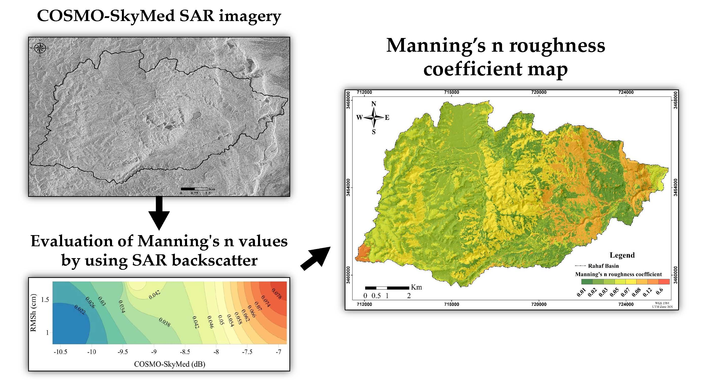
Evaluation of Manning’s n Roughness Coefficient in Arid Environments by Using SAR Backscatter

Abstract

1. Introduction
2. Methods
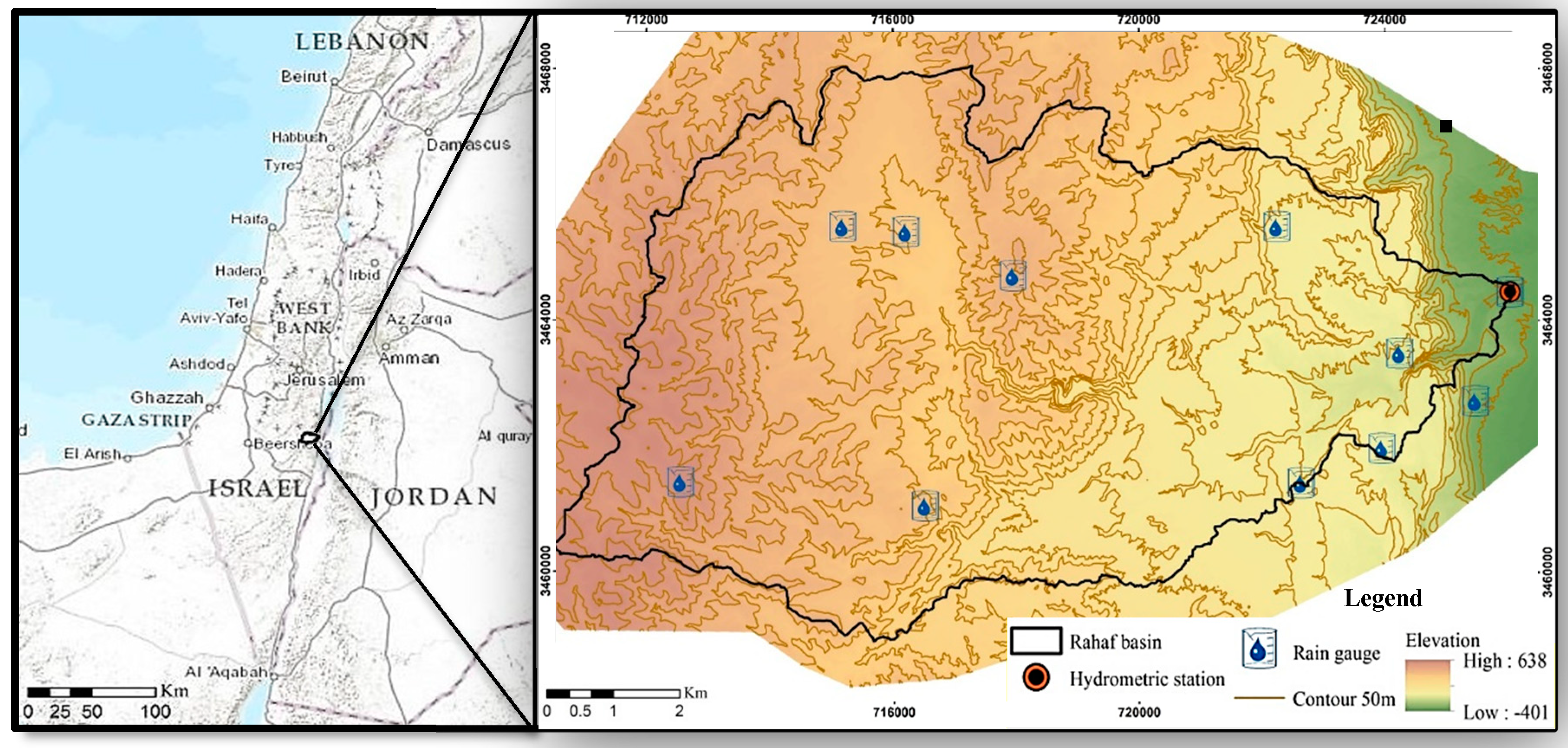
2.1. Study Area
2.2. SAR Data and Processing for Roughness Extraction
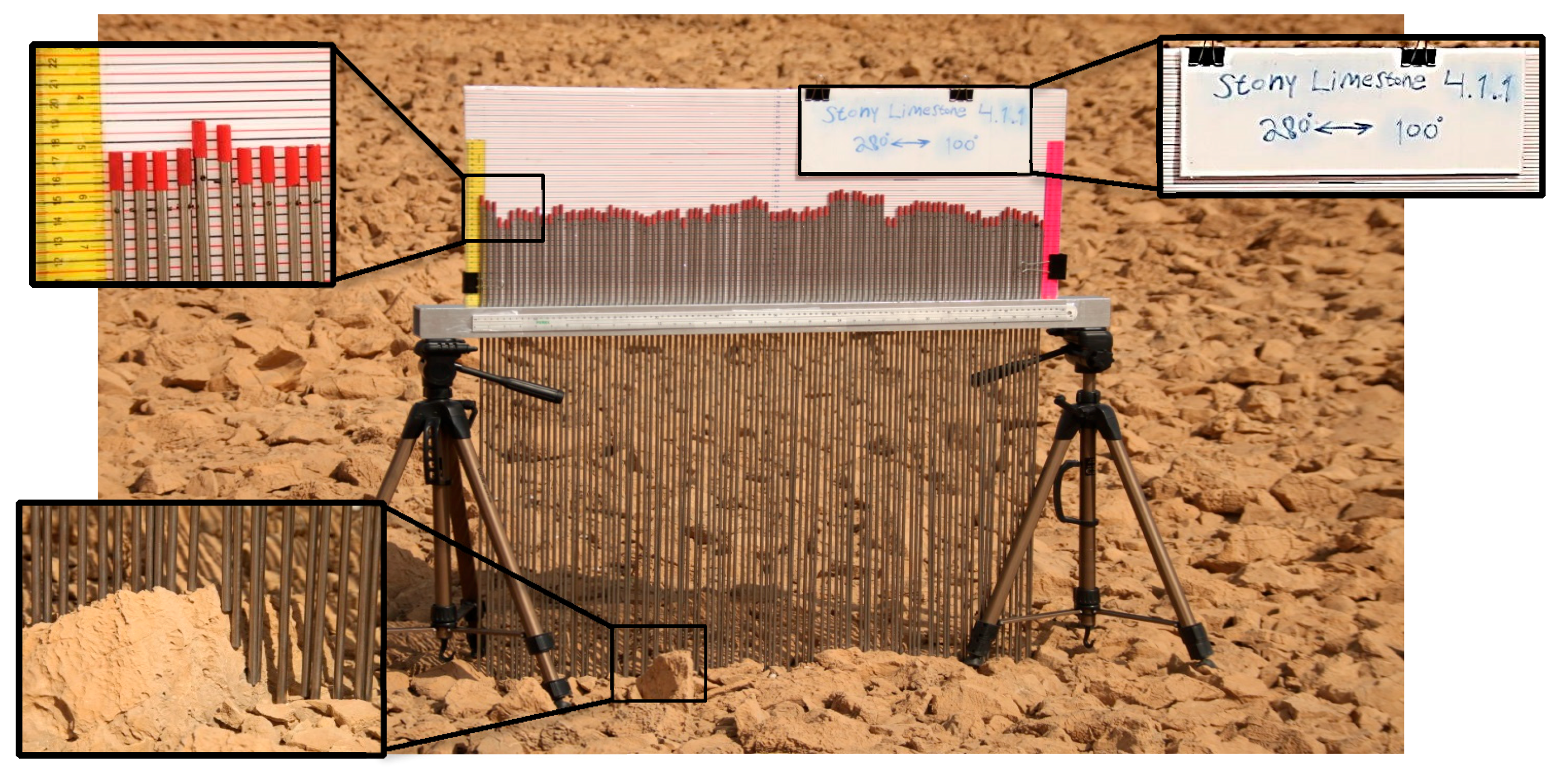
2.3. Field Roughness Measurements
3. Results
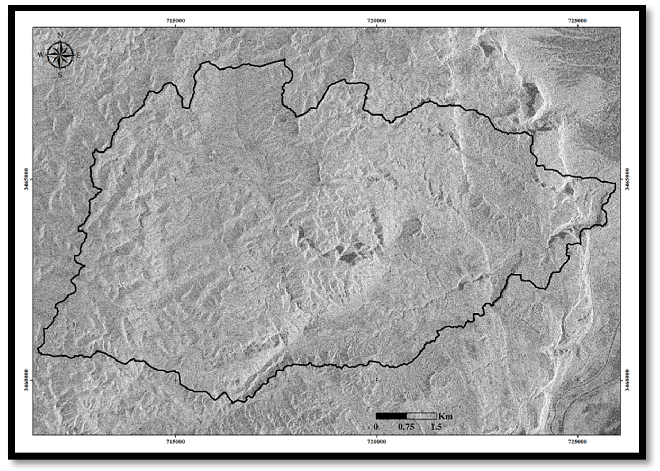
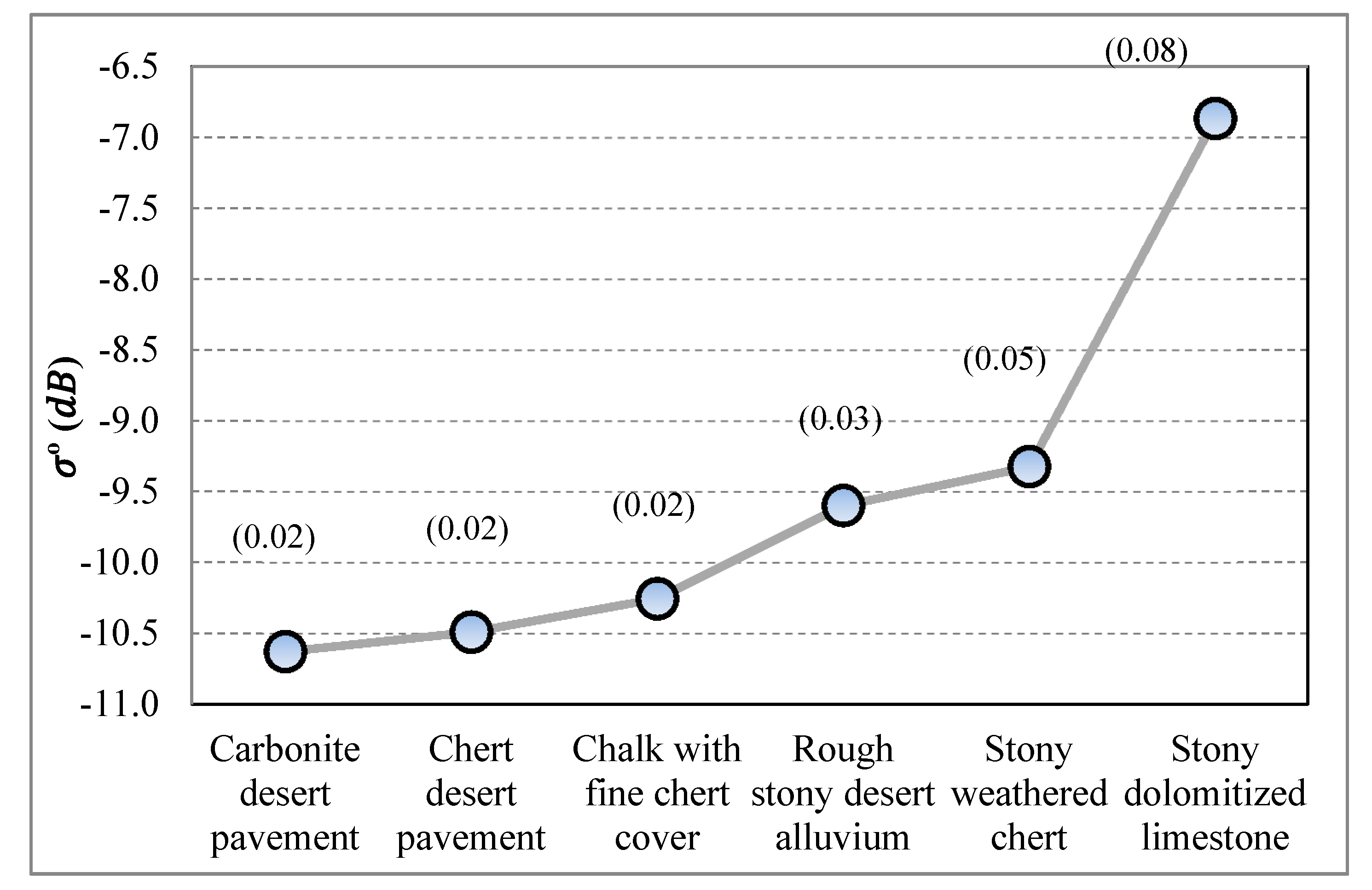
3.1. COSMO-SkyMed Imagery Analysis
3.2. Surface Roughness-Field Measurements
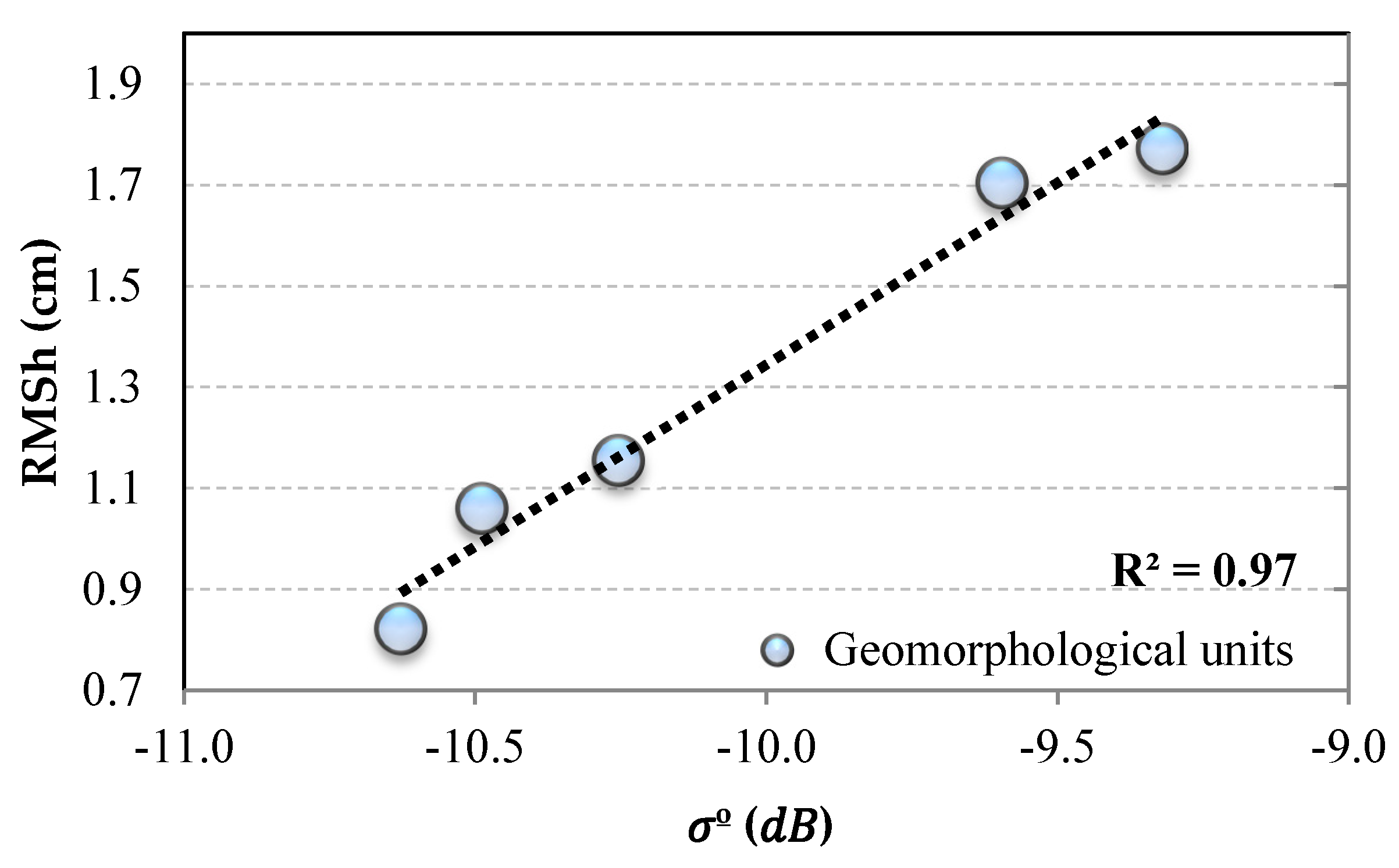
3.3. Correlation between the SAR Backscatter and Surface Roughness
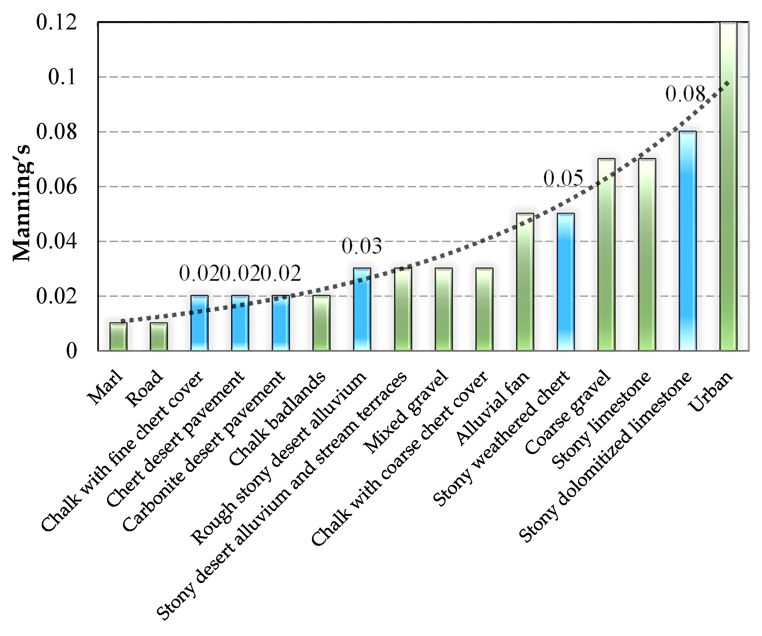
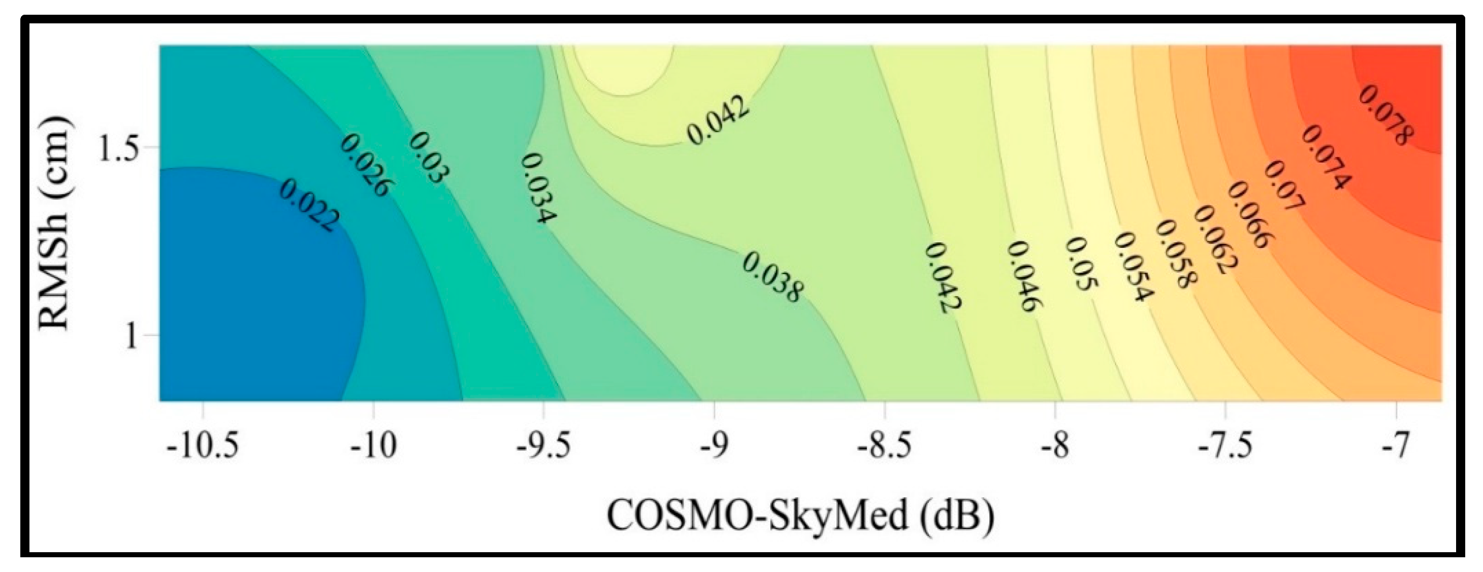
3.4. Using SAR Backscatter for the Evaluation of Manning’s n
4. Discussion
5. Conclusions
Author Contributions
Acknowledgments
Conflicts of Interest
References
- Hu, P.; Zhang, Q.; Shi, P.; Chen, B.; Fang, J. Flood-Induced Mortality Across the Globe: Spatiotemporal Pattern and Influencing Factors. Sci. Total Environ. 2018, 643, 171–182. [Google Scholar] [CrossRef] [PubMed]
- Paprotny, D.; Sebastian, A.; Morales-Nápoles, O.; Jonkman, S.N. Trends in Flood Losses in Europe over the Past 150 Years. Nat. Commun. 2018, 9, 1985. [Google Scholar] [CrossRef] [PubMed]
- Kundzewicz, Z.W.; Kanae, S.; Seneviratne, S.I.; Handmer, J.; Nicholls, N.; Peduzzi, P.; Mechler, R.; Bouwer, L.M.; Arnell, N.; Mach, K. Flood Risk and Climate Change: Global and Regional Perspectives. Hydrol. Sci. J. 2014, 59, 1–28. [Google Scholar] [CrossRef]
- Duan, W.; He, B.; Nover, D.; Fan, J.; Yang, G.; Chen, W.; Meng, H.; Liu, C. Floods and Associated Socioeconomic Damages in China Over the Last Century. Nat. Hazards 2016, 82, 401–413. [Google Scholar] [CrossRef]
- Yair, A.; Raz-Yassif, N. Hydrological Processes in a Small Arid Catchment: Scale Effects of Rainfall and Slope Length. Geomorphology 2004, 61, 155–169. [Google Scholar] [CrossRef]
- Singh, R. Real Time Flood Forecasting-Indian Experiences. In Hydrological Modelling in Arid and Semi-Arid Areas; Wheater, H., Sorooshian, S., Sharma, K., Eds.; Cambridge University Press: New York, NY, USA, 2008; pp. 139–156. [Google Scholar]
- Foody, G.M.; Ghoneim, E.M.; Arnell, N.W. Predicting Locations Sensitive to Flash Flooding in an Arid Environment. J. Hydrol. 2004, 292, 48–58. [Google Scholar] [CrossRef]
- Horton, R.E. Erosional Development of Streams and their Drainage Basins; Hydrophysical Approach to Quantitative Morphology. Geol. Soc. Am. Bull. 1945, 56, 275–370. [Google Scholar] [CrossRef]
- Michaud, J.; Sorooshian, S. Comparison of Simple versus Complex Distributed Runoff Models on a Midsized Semiarid Watershed. Water Resour. Res. 1994, 30, 593–605. [Google Scholar] [CrossRef]
- Engman, E.T. Roughness Coefficients for Routing Surface Runoff. J. Irrig. Drain. Eng. 1986, 112, 39–53. [Google Scholar] [CrossRef]
- Hernandez, M.; Miller, S.N.; Goodrich, D.C.; Goff, B.F.; Kepner, W.G.; Edmonds, C.M.; Jones, K.B. Modeling runoff response to land cover and rainfall spatial variability in semi-arid watersheds. In Monitoring Ecological Condition in the Western United States; Anonymous; Springer: Berlin, Germany, 2000; pp. 285–298. [Google Scholar]
- Greenbaum, N.; Margalit, A.; Schick, A.P.; Sharon, D.; Baker, V.R. A High Magnitude Storm and Flood in a Hyperarid Catchment, Nahal Zin, Negev Desert, Israel. Hydrol. Process. 1998, 12, 1–23. [Google Scholar] [CrossRef]
- Yair, A.; Kossovsky, A. Climate and Surface Properties: Hydrological Response of Small Arid and Semi-Arid Watersheds. Geomorphology 2002, 42, 43–57. [Google Scholar] [CrossRef]
- Lange, J. Dynamics of Transmission Losses in a Large Arid Stream Channel. J. Hydrol. 2005, 306, 112–126. [Google Scholar] [CrossRef]
- Cohen, H.; Laronne, J.B. High Rates of Sediment Transport by Flashfloods in the Southern Judean Desert, Israel. Hydrol. Process. 2005, 19, 1687–1702. [Google Scholar] [CrossRef]
- Vieux, B.E. Distributed Hydrologic Modeling Using GIS, 2nd ed.; Kluwer Academic: Dordrecht, The Netherlands, 2004. [Google Scholar]
- Forzieri, G.; Castelli, F.; Preti, F. Advances in Remote Sensing of Hydraulic Roughness. Int. J. Remote Sens. 2012, 33, 630–654. [Google Scholar] [CrossRef]
- Arcement, G.J.; Schneider, V.R. Guide for Selecting Manning’s Roughness Coefficients for Natural Channels and Flood Plains; United States Geological Survey Water-Supply Paper 2339; U.S. Geological Survey: Reston, VA, USA, 1989.
- El Bastawesy, M.; White, K.; Nasr, A. Integration of Remote Sensing and GIS for Modelling Flash Floods in Wadi Hudain Catchment, Egypt. Hydrol. Process. 2009, 23, 1359–1368. [Google Scholar] [CrossRef]
- Semmens, D.; Goodrich, D.; Unkrich, C.; Smith, R.; Woolhiser, D.; Miller, S. KINEROS2 and the AGWA modelling framework. In Hydrological Modelling in Arid and Semi-Arid Areas; Wheater, H., Sorooshian, S., Sharma, K., Eds.; Cambridge University Press: New York, NY, USA, 2008; pp. 49–68. [Google Scholar]
- Woolhiser, D.A.; Smith, R.; Goodrich, D.C. KINEROS: A Kinematic Runoff and Erosion Model; Documentation and User Manual; U.S. Department of Agriculture: Washington, DC, USA, 1990.
- Hagemann, M.; Gleason, C.; Durand, M. BAM: Bayesian AMHG-Manning Inference of Discharge using Remotely Sensed Stream Width, Slope, and Height. Water Resour. Res. 2017, 53, 9692–9707. [Google Scholar] [CrossRef]
- Pan, F.; Wang, C.; Xi, X. Constructing River Stage-Discharge Rating Curves using Remotely Sensed River Cross-Sectional Inundation Areas and River Bathymetry. J. Hydrol. 2016, 540, 670–687. [Google Scholar] [CrossRef]
- Thakur, P.K.; Aggarwal, S.; Aggarwal, S.; Jain, S. One-Dimensional Hydrodynamic Modeling of GLOF and Impact on Hydropower Projects in Dhauliganga River using Remote Sensing and GIS Applications. Nat. Hazards 2016, 83, 1057–1075. [Google Scholar] [CrossRef]
- Ullah, S.; Farooq, M.; Sarwar, T.; Tareen, M.J.; Wahid, M.A. Flood Modeling and Simulations using Hydrodynamic Model and ASTER DEM—A Case Study of Kalpani River. Arabian J. Geosci. 2016, 9, 439. [Google Scholar] [CrossRef]
- Wang, Y.; Yang, X. Sensitivity Analysis of the Surface Runoff Coefficient of HiPIMS in Simulating Flood Processes in a Large Basin. Water 2018, 10, 253. [Google Scholar] [CrossRef]
- Forzieri, G.; Degetto, M.; Righetti, M.; Castelli, F.; Preti, F. Satellite Multispectral Data for Improved Floodplain Roughness Modelling. J. Hydrol. 2011, 407, 41–57. [Google Scholar] [CrossRef]
- Rahman, M.; Moran, M.; Thoma, D.; Bryant, R.; Holifield Collins, C.; Jackson, T.; Orr, B.; Tischler, M. Mapping Surface Roughness and Soil Moisture using Multi-Angle Radar Imagery without Ancillary Data. Remote Sens. Environ. 2008, 112, 391–402. [Google Scholar] [CrossRef]
- Evans, D.L.; Farr, T.G.; Van Zyl, J.J. Estimates of Surface Roughness Derived from Synthetic Aperture Radar (SAR) Data. IEEE Trans. Geosci. Remote Sens. 1992, 30, 382–389. [Google Scholar] [CrossRef]
- Verhoest, N.E.; Lievens, H.; Wagner, W.; Álvarez-Mozos, J.; Moran, M.S.; Mattia, F. On the Soil Roughness Parameterization Problem in Soil Moisture Retrieval of Bare Surfaces from Synthetic Aperture Radar. Sensors 2008, 8, 4213–4248. [Google Scholar] [CrossRef] [PubMed]
- Marzahn, P.; Ludwig, R. On the Derivation of Soil Surface Roughness from Multi Parametric PolSAR Data and its Potential for Hydrological Modeling. Hydrol. Earth Syst. Sci. 2009, 13, 381. [Google Scholar] [CrossRef]
- Baghdadi, N.; Paillou, P.; Grandjean, G.; Dubois, P.; Davidson, M. Relationship between Profile Length and Roughness Variables for Natural Surfaces. Int. J. Remote Sens. 2000, 21, 3375–3381. [Google Scholar] [CrossRef]
- Hetz, G.; Mushkin, A.; Blumberg, D.G.; Baer, G.; Ginat, H. Estimating the Age of Desert Alluvial Surfaces with Spaceborne Radar Data. Remote Sens. Environ. 2016, 184, 288–301. [Google Scholar] [CrossRef]
- Abdelsalam, M.G.; Robinson, C.; El-Baz, F.; Stern, R.J. Applications of Orbital Imaging Radar for Geologic Studies in Arid Regions: The Saharan Testimony. Photogramm. Eng. Remote Sens. 2000, 66, 717–726. [Google Scholar]
- Blumberg, D.G.; Greeley, R. Field Studies of Aerodynamic Roughness Length. J. Arid Environ. 1993, 25, 39–48. [Google Scholar] [CrossRef]
- Xia, Z.; Henderson, F.M. Understanding the Relationships between Radar Response Patterns and the Bio-and Geophysical Parameters of Urban Areas. IEEE Trans. Geosci. Remote Sens. 1997, 35, 93–101. [Google Scholar]
- Blumberg, D.G.; Freilikher, V. Soil Water-Content and Surface Roughness Retrieval using ERS-2 SAR Data in the Negev Desert, Israel. J. Arid Environ. 2001, 49, 449–464. [Google Scholar] [CrossRef]
- Weeks, R.; Smith, M.; Pak, K.; Li, W.; Gillespie, A.; Gustafson, B. Surface Roughness, Radar Backscatter, and Visible and Near-Infrared Reflectance in Death Valley, California. J. Geophys. Res. 1996, 101, 23077–23090. [Google Scholar] [CrossRef]
- Weeks, R.; Smith, M.; Pak, K.; Gillespie, A. Inversions of SIR-C and AIRSAR Data for the Roughness of Geological Surfaces. Remote Sens. Environ. 1997, 59, 383–396. [Google Scholar] [CrossRef]
- Campbell, B.A.; Campbell, D.B. Analysis of Volcanic Surface Morphology on Venus from Comparison of Arecibo, Magellan, and Terrestrial Airborne Radar Data. J. Geophys. Res. Planets 1992, 97, 16293–16314. [Google Scholar] [CrossRef]
- Deroin, J.; Simonin, A. An Empirical Model for Interpreting the Relationship between Backscattering and Arid Land Surface Roughness as seen with the SAR. IEEE Trans. Geosci. Remote Sens. 1997, 35, 86–92. [Google Scholar] [CrossRef]
- Cohen, H. Floods and Sediment Transport in Dryland Rivers. Ph.D. Thesis, Ben-Gurion University of the Negev, Beersheba, Israel, 2005. [Google Scholar]
- Cohen, H.; Laronne, B.J. Rainfall-Runoff Relations in Arid Environment and Applications for Floods and Sediment Transport Forecast; Department of Geography and Environmental Development, Ben-Gurion University of the Negev: Beer-Sheva, Israel, 2011. [Google Scholar]
- Farr, T.G. Guide to Magellan Image Interpretation; Chapter 5: Radar Interactions with Geologic Surfaces; Jet Propulsion Laboratory, California Institute of Technology: La Cañada Flintridge, CA, USA, 1993. [Google Scholar]
- Wu, X.; Yu, D.; Chen, Z.; Wilby, R.L. An Evaluation of the Impacts of Land Surface Modification, Storm Sewer Development, and Rainfall Variation on Waterlogging Risk in Shanghai. Nat. Hazards 2012, 63, 305–323. [Google Scholar] [CrossRef]
- Bryant, R.; Moran, M.S.; Thoma, D.P.; Holifield Collins, C.D.; Skirvin, S.; Rahman, M.; Slocum, K.; Starks, P.; Bosch, D.; Gonzalez Dugo, M.P. Measuring Surface Roughness Height to Parameterize Radar Backscatter Models for Retrieval of Surface Soil Moisture. IEEE Geosci. Remote Sens. Lett. 2007, 4, 137–141. [Google Scholar] [CrossRef]
- Oh, Y.; Sarabandi, K.; Ulaby, F.T. An Empirical Model and an Inversion Technique for Radar Scattering from Bare Soil Surfaces. IEEE Trans. Geosci. Remote Sens. 1992, 30, 370–381. [Google Scholar] [CrossRef]
- Mushkin, A.; Sagy, A.; Trabelci, E.; Amit, R.; Porat, N. Measuring the Time and Scale-Dependency of Subaerial Rock Weathering Rates Over Geologic Time Scales with Ground-Based Lidar. Geology 2014, 42, 1063–1066. [Google Scholar] [CrossRef]
- Turner, R.; Panciera, R.; Tanase, M.A.; Lowell, K.; Hacker, J.M.; Walker, J.P. Estimation of Soil Surface Roughness of Agricultural Soils using Airborne LiDAR. Remote Sens. Environ. 2014, 140, 107–117. [Google Scholar] [CrossRef]
- Mattia, F.; Le Toan, T.; Souyris, J.; De Carolis, C.; Floury, N.; Posa, F.; Pasquariello, N. The Effect of Surface Roughness on Multifrequency Polarimetric SAR Data. IEEE Trans. Geosci. Remote Sens. 1997, 35, 954–966. [Google Scholar] [CrossRef]
- Alvarez-Mozos, J.; Gonzalez-Audicana, M.; Casali, J.; Larranaga, A. Effective Versus Measured Correlation Length for Radar-Based Surface Soil Moisture Retrieval. Int. J. Remote Sens. 2008, 29, 5397–5408. [Google Scholar] [CrossRef]
- Raz, E. The Geology of the Judean Desert. Master’s Thesis, The Hebrew University of Jerusalem, Jerusalem, Israel, 1983. [Google Scholar]
- Smith, M.; Asal, F.; Priestnall, G. The use of Photogrammetry and Lidar for Landscape Roughness Estimation in Hydrodynamic Studies. ISPRS XXXB Part B 2004, 3, 714–719. [Google Scholar]
- Horritt, M.; Di Baldassarre, G.; Bates, P.; Brath, A. Comparing the Performance of a 2-D Finite Element and a 2-D Finite Volume Model of Floodplain Inundation using Airborne SAR Imagery. Hydrol. Process. 2007, 21, 2745–2759. [Google Scholar] [CrossRef]
- Tarpanelli, A.; Brocca, L.; Melone, F.; Moramarco, T. Hydraulic Modelling Calibration in Small Rivers by using Coarse Resolution Synthetic Aperture Radar Imagery. Hydrol. Process. 2013, 27, 1321–1330. [Google Scholar] [CrossRef]
- Mtamba, J.; van der Velde, R.; Ndomba, P.; Zoltán, V.; Mtalo, F. Use of Radarsat-2 and Landsat TM Images for Spatial Parameterization of Manning’s Roughness Coefficient in Hydraulic Modeling. Remote Sens. 2015, 7, 836–864. [Google Scholar] [CrossRef]
- Simoes, N.E.d.C. Urban Pluvial Flood Forecasting. Ph.D. Thesis, Imperial College London, London, UK, 2012. [Google Scholar]
- Houston, D.; Werrity, A.; Bassett, D.; Geddes, A.; Hoolachan, A.; McMillan, M. Pluvial (Rain-Related) Flooding in Urban Areas: The Invisible Hazard; Joseph Rowntree Foundation: York, UK, 2011. [Google Scholar]
- Jiang, Y.; Zevenbergen, C.; Ma, Y. Urban Pluvial Flooding and Stormwater Management: A Contemporary Review of China’s Challenges and “sponge Cities” Strategy. Environ. Sci. Policy 2018, 80, 132–143. [Google Scholar] [CrossRef]
- Acosta-Coll, M.; Ballester-Merelo, F.; Martinez-Peiro, M.; De la Hoz-Franco, E. Real-Time Early Warning System Design for Pluvial Flash Floods-A Review. Sensors 2018, 18, 2255. [Google Scholar] [CrossRef] [PubMed]


© 2018 by the authors. Licensee MDPI, Basel, Switzerland. This article is an open access article distributed under the terms and conditions of the Creative Commons Attribution (CC BY) license (http://creativecommons.org/licenses/by/4.0/).
Share and Cite
Sadeh, Y.; Cohen, H.; Maman, S.; Blumberg, D.G. Evaluation of Manning’s n Roughness Coefficient in Arid Environments by Using SAR Backscatter. Remote Sens. 2018, 10, 1505. https://doi.org/10.3390/rs10101505
Sadeh Y, Cohen H, Maman S, Blumberg DG. Evaluation of Manning’s n Roughness Coefficient in Arid Environments by Using SAR Backscatter. Remote Sensing. 2018; 10(10):1505. https://doi.org/10.3390/rs10101505
Chicago/Turabian StyleSadeh, Yuval, Hai Cohen, Shimrit Maman, and Dan G. Blumberg. 2018. "Evaluation of Manning’s n Roughness Coefficient in Arid Environments by Using SAR Backscatter" Remote Sensing 10, no. 10: 1505. https://doi.org/10.3390/rs10101505
APA StyleSadeh, Y., Cohen, H., Maman, S., & Blumberg, D. G. (2018). Evaluation of Manning’s n Roughness Coefficient in Arid Environments by Using SAR Backscatter. Remote Sensing, 10(10), 1505. https://doi.org/10.3390/rs10101505