Spectral Invariant Provides a Practical Modeling Approach for Future Biophysical Variable Estimations

Abstract

This paper presents a simple radiative transfer model based on spectral invariant properties (SIP). The canopy structure parameters, including the leaf angle distribution and multi-angular clumping index, are explicitly described in the SIP model. The SIP model has been evaluated on its bidirectional reflectance factor (BRF) in the angular space at the radiation transfer model intercomparison platform, and in the spectrum space by the PROSPECT+SAIL (PROSAIL) model. The simulations of BRF by SIP agreed well with the reference values in both the angular space and spectrum space, with a root-mean-square-error (RMSE) of 0.006. When compared with the widely-used Soil-Canopy Observation of Photochemistry and Energy fluxes (SCOPE) model on fPAR, the RMSE was 0.006 and the R² was 0.99, which shows a high accuracy. This study also suggests the newly proposed vegetation index, the near-infrared (NIR) reflectance of vegetation (NIRv), was a good linear approximation of the canopy structure parameter, the directional area scattering factor (DASF), with an R² of 0.99. NIRv was not influenced much by the soil background contribution, but was sensitive to the leaf inclination angle. The sensitivity of NIRv to canopy structure and the robustness of NIRv to the soil background suggest NIRv is a promising index in future biophysical variable estimations with the support of the SIP model, especially for the Deep Space Climate Observatory (DSCOVR) Earth Polychromatic Imaging Camera (EPIC) observations near the hot spot directions.

1. Introduction

Canopy reflectance models have been widely used as the forward model for biophysical variable estimations, e.g., leaf area index (LAI), fractional vegetation cover (FVC) and the fraction of absorbed photosynthetically active radiation (fPAR) [1,2,3,4,5]. However, there are a large variety of models to be selected, depending on the complexity of the canopy structure [6,7,8]. For horizontally homogeneous canopies, e.g., cropland and grassland, there are 1D radiative transfer (RT) models, such as the PROSPECT+SAIL (PROSAIL) model and the two-layer Markov chain canopy reflectance (ACRM) model [9,10]; for discontinuous canopies, e.g., sparse forest, there are geometric–optical (GO)-based or hybrid models, such as the five-scale model, FRT model and SRTE model [11,12,13]. There is a lack of a simple unified RT model that is suitable for both continuous and discontinuous canopies with different heterogeneities [14,15]. The newly launched Deep Space Climate Observatory (DSCOVR) with the sensor Earth Polychromatic Imaging Camera (EPIC) provides unique near hot spot observations with a sub-hourly temporal frequency, which requires accurate RT forwarding modeling near the hot spot region for biophysical variable estimations [16].

Spectral invariant theory simplifies the radiative transfer process by decoupling the canopy structure and leaf optics [17]. There are three key spectral invariant parameters to describe the canopy structure: the canopy interceptance $i_0$, recollision probability $p$ and escape probability $\rho$ [18,19,20]. The canopy interceptance $i_0$ is the fraction of photons that are intercepted by leaves in the canopy; the recollision probability $p$ is defined as the probability that a photon scattered from a leaf in a canopy will interact within the canopy again; the escape probability $\rho$ is defined as the probability that a scattered photon will escape the canopy. By the three wavelength-independent parameters, it is no longer necessary to use the successive orders of scattering approximation (SOSA) method for the multiple scattering calculation, which is usually iteration-based and time-consuming [21]. The spectral invariant has recently been used in the remotely sensed albedo [22], fPAR [23] and sunlit LAI estimations [22,23,24]. However, there are still several aspects of the spectral invariant that need to be improved for future biophysical variable estimations.

The first aspect is how to explicitly describe the spectral invariant by canopy structure parameters, including the leaf angle distribution (LAD) and clumping index (CI) [25,26]. Only by linking the canopy structure parameters with the abstract spectral invariant can we estimate the canopy structure parameters from remotely sensed observations. Stenberg [27] found a simple analytical formula for the relationship between LAI and recollision probability, while LAD and CI are still important to explicitly account for. In fact, LAD is one of the key parameters that determine the angular distribution of the reflected photons. It is common to assume the LAD as spherical distribution or a given type for each biome [17], while canopy-level studies have shown that such an assumption can result in as much as a 47% underestimation in LAI if the true LAD distribution is better characterized as planophile [28]. Besides this, accounting for the clumping effects is the key to making the 1D RT model applicable to discontinuous canopies. CI measurements are primarily recorded as hemispherically integrated CI [29], despite the fact that CI strongly varies with the view zenith angle [30,31,32]. The angular variation effect of CI is still important to describe in the RT process.

The second challenge is how to explicitly account for the hot spot effect in the RT process by the spectral invariant, which is due to the finite size of the leaf element [33]. The hot spot effect is that the reflectance reaches the local maximum when the view and solar direction coincide, because there is no shadow in view. Thus, the single scattering contribution by the first-order escape probability needs to be treated separately. The simple semi-physical parameterization (PARAS) model, which is forest spectral invariant-based, does not include the hot spot effect yet [34]. Recently Yang, et al. [24] began to incorporate the hot spot phenomenon by separating the escape probability of sunlit leaves and shaded leaves. Up to now, as far as we know, the spectral invariant-based bidirectional reflectance factor (BRF) models still have not been validated at the radiation transfer model intercomparison (RAMI) online model checker (ROMC) platform [35].

The last aspect is how to describe the multiple scattering between vegetation and soil and reduce the soil contamination in the biophysical variable estimations. The multiple scattering between vegetation and soil can still make a considerable contribution to the BRF when the LAI is low and the soil is bright, e.g., sparse forest with snow background, while this effect still has not been accounted for in the PARAS model [34]. Besides this, the direct extraction of recollision probability and directional area scattering factor (DASF) by the BRF-fitting approach assumes soil background effects are negligible (black soil problem) [18,36]. If not, a full RT model by stochastic radiative transfer equation (SRTE), would be used to remove the soil contribution (soil problem), which reduces the simplicity of the spectral invariant approach [13,24]. In fact, DASF is a canopy structure parameter and is equal to the canopy BRF when there is no soil background contribution and the leaves have no absorption (leaf albedo w = 1). Thus, it is important to find a simple index that can be directly extracted from BRF observations, and at the same time is robust to soil brightness in the biophysical variable estimations, e.g., the newly developed vegetation index, the near-infrared (NIR) reflectance of vegetation (NIRv) [37]. NIRv is the product of the total NIR reflectance and the normalized difference vegetation index (NDVI), and has been shown to be insensitive to soil background contribution [37]. By NIRv, we do not need to account for the single scattering contribution of the soil and the photon interactions between vegetation and soil, and this is therefore promising for future biophysical estimations.

To address the above three challenges, we develop a simple RT model based on spectral invariant properties (SIP) which explicitly describes the leaf angle distribution (LAD) and clumping index (CI) and treats the single scattering contribution separately. Then, we evaluate the SIP model of BRF by the RAMI platform in the angular space [35], compare the SIP model with the PROSAIL model in the spectrum space [10], and evaluate the SIP model of fPAR by the Soil-Canopy Observation of Photochemistry and Energy fluxes (SCOPE) model [38], a widely accepted model that can directly simulate fPAR as the output. The input parameters are varied at different canopy structures, solar angles, and soil backgrounds. Then, the impact of the soil effect on DASF calculation has been evaluated by the proposed SIP model. Finally, the impact of LAD on BRF and NIRv has been evaluated.

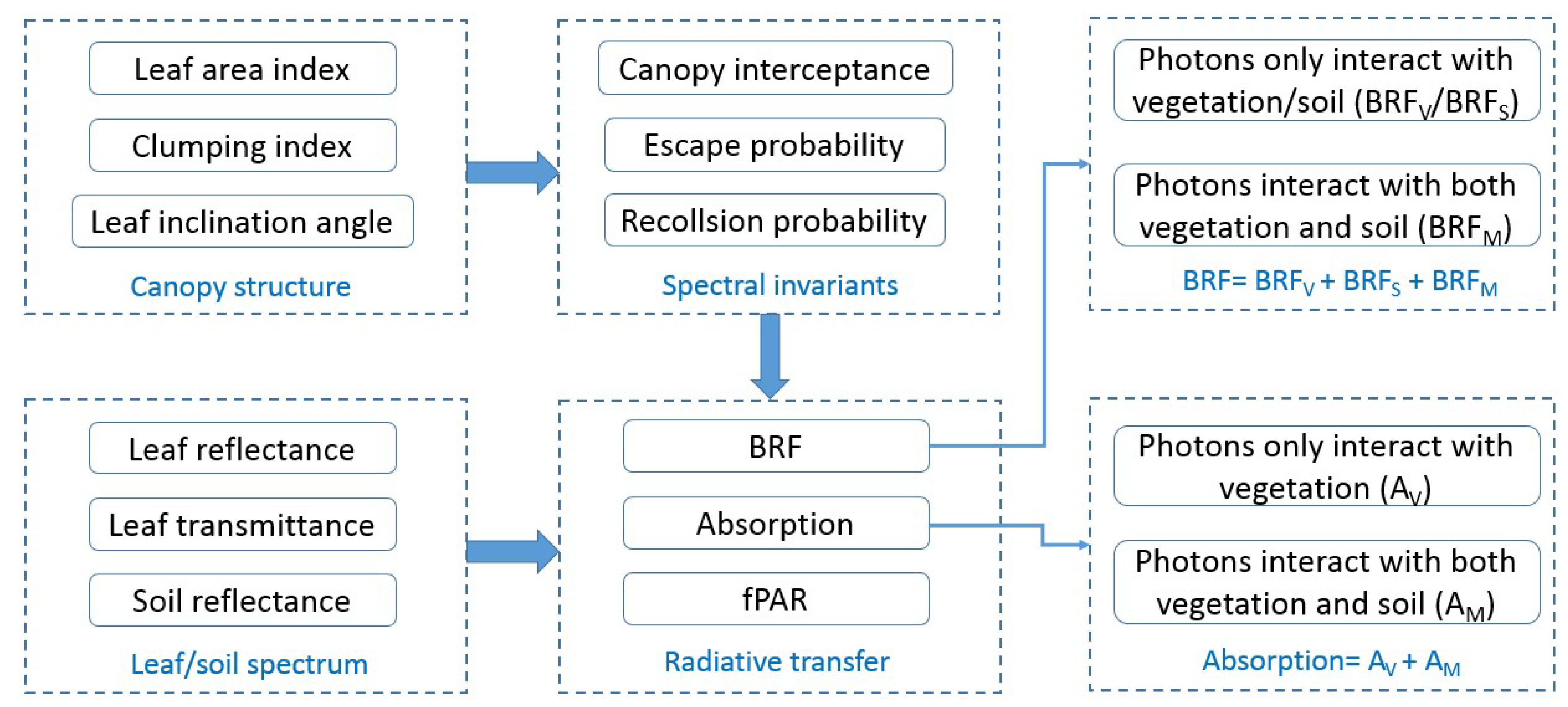
2. Model Description

Accounting for the fact that the first-order escape probability has a stronger anisotropic effect than high-order ones [24], the SIP model proposed in this study adopts the method of calculating the single scattering contribution from the PROSAIL model [10], but meanwhile explicitly describes the clumping effects and the leaf angle distribution. The multiple scattering within the canopy, and the interactions between the canopy and the soil, are calculated in the framework of the spectral invariant, which has the advantage of simplicity compared with the SOSA method [21]. The framework of the SIP model is in Figure 1, and detailed descriptions of each item are in Section 2 as follows.

2.1. BRF of the Vegetation-Soil System

The BRF of the vegetation–soil system at the wavelength of $\lambda$ and at the solar-sensor geometry $\mathsf{\Omega }$ contains three components:

$$BRF\left(\lambda ,\mathsf{\Omega }\right) = BR{F}_V\left(\lambda ,\mathsf{\Omega }\right)+BR{F}_S\left(\lambda ,\mathsf{\Omega }\right)+BR{F}_M\left(\lambda ,\mathsf{\Omega }\right)$$

(1)

where $BR{F}_V$ is the contribution of the photons from vegetation with no interaction with the soil background, $BR{F}_S$ is the single scattering contribution of the photons from soil background with no interaction with the vegetation, and $BR{F}_M$ is the multiple scattering contribution of the photons between the vegetation and soil. The solar-sensor geometry $\mathsf{\Omega }$ contains the solar-target geometry and target-sensor geometry, and both of them can be described by the zenith angle and azimuth angle.

(1) Photons which only interact with the vegetation ($BR{F}_V$)

$BR{F}_V$ comprises the single scattering of the vegetation ($BR{F}_{V1}$) and multiple scattering within the vegetation with no interaction with the soil ($BR{F}_{VM}$):

$$BR{F}_V\left(\lambda ,\mathsf{\Omega }\right) = BR{F}_{V1}\left(\lambda ,\mathsf{\Omega }\right)+BR{F}_{VM}\left(\lambda ,\mathsf{\Omega }\right)$$

(2)

where $BR{F}_{V1}$ can be derived as

$$BR{F}_{V1}\left(\lambda ,\mathsf{\Omega }\right)=\overline{w_{so}\left(\lambda ,\mathsf{\Omega },{\theta }_l\right)}·{\int }_0^H{u}_L\left(z\right)·P_{so}\left(\mathsf{\Omega },z\right)dz$$

(3)

$w_{so}$ is the average bidirectional scattering coefficient in the PROSAIL model integrated over all the leaf inclination angles from 0° to 90° [10], which is a function of leaf reflectance/transmittance at the wavelength of $\lambda$, leaf inclination angle ${\theta }_l$, and the solar-sensor geometry $\mathsf{\Omega }$. $u_L$ is the leaf area density $(m^2/m^3)$, $H$ is the canopy height, and $P_{so}\left(\mathsf{\Omega },z\right)$ is the bidirectional gap fraction at height z, which is a function of the directional gap fraction at height z with the solar zenith angle ${\theta }_s$ ($P_s$) and the view zenith angle ${\theta }_o$($P_o$.), and the hot spot correction function $C_{HS}=C_{HS}\left(\xi ,s,s^{\prime }\right)=\exp \left[\sqrt{\tau s{\tau }^{\prime }{s}^{\prime }}\frac{1-\exp \left(-k_l{S}_{AB}\right)}{k_l{S}_{AB}}\right]$ at height z with a phase angle $\xi$ of the solar-sensor direction [33]. Here $\tau$ and ${\tau }^{\prime }$ are the extinction coefficients in the solar and view directions, respectively; $s$ and $s^{\prime }$ are the optical lengths intersected the vegetated component in the solar and view directions, respectively; and $\xi$ is the scattering phase angle between the solar and view directions. $k_l=1/s_L$, and $s_L$ is the characteristic linear dimension of the leaves [33]. $S_{AB}$ is the distance between the two points A and B where the solar and the observation rays penetrate into the canopy [15], and $S_{AB}$ can be computed as $S_{AB}=\sqrt{s^2+{s^{\prime }}^2-2s{s}^{\prime }cos\xi }$, where $\xi$ can be calculated from the solar/view zenith angle ${\theta }_s$ and ${\theta }_o$, respectively, and the solar/view azimuth angle ${\phi }_s$ and ${\phi }_o$, respectively, as $cos\xi =cos{\theta }_{s}cos{\theta }_o+sin{\theta }_{s}sin{\theta }_o\cos \left({\phi }_s-{\phi }_o\right)$ [15,33].

$$P_{so}\left(\mathsf{\Omega },z\right) = P_s\left({\theta }_s,z\right)·P_o\left({\theta }_o,z\right)·C_{HS}\left(\xi ,z\right)$$

(4)

The directional gap fraction $P_s\left({\theta }_s,z\right)$ at height z with the solar zenith angle ${\theta }_s$ can be described as

$$P_s\left({\theta }_s,z\right) = \exp [-\frac{G\left({\theta }_s\right)}{{\mu }_s}·LAI\left(z\right)·CI\left({\theta }_s\right)]$$

(5)

where $G\left({\theta }_s\right)$ is the leaf projection function at the solar direction and is a function of the leaf inclination angle ${\theta }_l$, ${\mu }_s = cos{\theta }_s$, $LAI\left(z\right)$ is the culmulative LAI at height z from the top, $LAI\left(H\right)$ is the canopy LAI, and $CI\left({\theta }_s\right)$ is the clumping index at the solar zenith angle ${\theta }_s$. When we replace the solar zenith angle ${\theta }_s$ in Equation (5) by the view zenith angle ${\theta }_o$, we can get the directional gap fraction $P_o\left({\theta }_o,z\right)$ at height z with the view zenith angle ${\theta }_o$. By Equations (3) and (5), the leaf inclination angle and multi-angular clumping index have been explicitly accounted for in the SIP model.

The multiple scattering within the vegetation $BR{F}_{VM}$ can be derived by the spectral invariant as

$$\begin{gathered} BR{F}_{VM}\left(\lambda ,\mathsf{\Omega }\right) = i_0·\omega \left(\lambda \right)·\left[p\omega \left(\lambda \right)·\rho \left(\mathsf{\Omega }\right)+p\omega \left(\lambda \right)·p\omega \left(\lambda \right)·\rho \left(\mathsf{\Omega }\right)+\cdots \right] \\ =i_0\omega \left(\lambda \right)\frac{p\omega \left(\lambda \right)\rho \left(\mathsf{\Omega }\right)}{1-p\omega \left(\lambda \right)} \end{gathered}$$

(6)

where $\omega \left(\lambda \right)$ is the leaf albedo, and the method for linking the canopy structure parameters with the canopy directional interceptance $i_0$, the directional escape probability $\rho \left(\mathsf{\Omega }\right)$ and recollision probability $p$ will be described in Section 2.4.

(2) Photons which only interact with the soil ($BR{F}_S$)

In fact, $BR{F}_S$ is the contribution of the sunlit soil, and can be described as

$$BR{F}_S\left(\lambda ,\mathsf{\Omega }\right) = K_g·{\rho }_G\left(\lambda \right)$$

(7)

where ${\rho }_G\left(\lambda \right)$ is the soil reflectance, and $K_g$ is the fraction of visible sunlit soil in view, which is equal to the bidirectional gap fraction at the bottom of the canopy $P_{so}\left(\mathsf{\Omega },H\right)$ in Equation (4).

(3) Photons which interact with the both the vegetation and soil ($BR{F}_M$)

$BR{F}_M$ is the multiple scattering between vegetation and soil, and can be described as

$$BR{F}_M\left(\lambda ,\mathsf{\Omega }\right) = \frac{{\rho }_G\left(\lambda \right)}{1-{\rho }_G\left(\lambda \right)·R_{dn}\left(\lambda \right)}·T_{dn}\left(\lambda \right)·T_{up}\left(\lambda ,\mathsf{\Omega }\right)-t_0·{\rho }_G\left(\lambda \right)·t_0^{dif}\left(\mathsf{\Omega }\right)$$

(8)

where $T_{dn}$ and $T_{up}$ are the canopy downwelling and upward transmittance which will be described in Section 2.3, $R_{dn}\left(\lambda \right)$ is the albedo in the downward direction under isotropic diffuse illumination from the bottom of the canopy, $t_0 = 1-i_0$, and $t_0^{dif}$ is the canopy directional transmittance under diffuse radiation illumination.

2.2. Absorption of the Vegetation and fPAR

The total photons absorbed by the vegetation comprise two components:

$$A\left(\lambda \right) = A_V\left(\lambda \right)+A_M\left(\lambda \right)$$

(9)

$A_V\left(\lambda \right)$ represents the absorbed photons that only interact with the vegetation [17]:

$$A_V\left(\lambda \right) = i_0\frac{1-\omega \left(\lambda \right)}{1-p\omega \left(\lambda \right)}$$

(10)

$A_M\left(\lambda \right)$ represents the photons that interact with both the vegetation and the soil, but are finally absorbed by the vegetation:

$$A_M\left(\lambda \right) = \frac{{\rho }_G\left(\lambda \right)}{1-{\rho }_G\left(\lambda \right)·R_{dn}\left(\lambda \right)}·T_{dn}\left(\lambda \right)·A_{up}\left(\lambda \right)$$

(11)

where $R_{dn}\left(\lambda \right)$ is the albedo in the downward direction under isotropic diffuse illumination from the bottom of the canopy, and $A_{up}\left(\lambda \right)$ is the corresponding absorption by vegetation. The two terms will be described in Section 2.3.

Finally, fPAR is the integration of the vegetation absorption $A\left(\lambda \right)$ and the incoming solar irradiance $R_{in}\left(\lambda \right)$ across the range 400 nm–700 nm:

$$fPAR = \frac{{\int }_{400nm}^{700nm}{R}_{in}\left(\lambda \right)·A\left(\lambda \right)}{{\int }_{400nm}^{700nm}{R}_{in}\left(\lambda \right)}$$

(12)

2.3. Canopy Radiation Transfer Terms by Spectral Invariant

The canopy level radiation transfer terms in Equations (8) and (11) will be described by the spectral invariant in this section. The canopy downwelling transmittance with black soil background in Equation (8) can be described as

$$\begin{gathered} T_{dn}\left(\lambda \right) = t_0+i_0·\omega \left(\lambda \right)·\left[{\tau }^{hemi}+p\omega \left(\lambda \right)·{\tau }^{hemi}+\cdots \right] \\ =t_0+i_0\omega \left(\lambda \right)\frac{{\tau }^{hemi}}{1-p\omega \left(\lambda \right)} \end{gathered}$$

(13)

where ${\tau }^{hemi}$ is the hemispherical escape probability in the downward direction, that will be described in Section 2.4. The canopy upward transmittance under isotropic illumination from the bottom of the canopy, but with black soil background in Equation (8), can be described as

$$\begin{gathered} T_{up}\left(\lambda ,\mathsf{\Omega }\right) = t_0^{dif}\left(\mathsf{\Omega }\right)+i_D·\omega \left(\lambda \right)·\left[\tau \left(\mathsf{\Omega }\right)+p\omega \left(\lambda \right)·\tau \left(\mathsf{\Omega }\right)+\cdots \right] \\ =t_0^{dif}\left(\mathsf{\Omega }\right)+i_D\omega \left(\lambda \right)\frac{\tau \left(\mathsf{\Omega }\right)}{1-p\omega \left(\lambda \right)} \end{gathered}$$

(14)

where $t_0^{dif}$ is the canopy directional transmittance under diffuse radiation illumination, and $i_D$ is the hemispherical canopy interceptance under diffuse radiation illumination, which will be described in Section 2.4.

The albedo in the downward direction under isotropic diffuse illumination from the bottom of the canopy, but with black soil background in Equation (11), can be described as

$$\begin{gathered} R_{dn}\left(\lambda \right) = i_D·\omega \left(\lambda \right)· \left[{\rho }^{hemi}+p\omega \left(\lambda \right)·{\rho }^{hemi}+\cdots \right] \\ = i_D\omega \left(\lambda \right)\frac{{\rho }^{hemi}}{1-p\omega \left(\lambda \right)} \end{gathered}$$

(15)

where ${\rho }^{hemi}$ is the hemispherical escape probability in the upward direction that will be described in Section 2.4. Similar to Equation (10), the absorption by vegetation under isotropic diffuse illumination from the bottom of the canopy, but with black soil background in Equation (11), can be described as

$$A_{up}\left(\lambda \right) = i_D\frac{1-\omega \left(\lambda \right)}{1-p\omega \left(\lambda \right)}$$

(16)

2.4. Analytical Formula of Spectral Invariant by Canopy Structure

(1) Canopy interceptance

The directional canopy interceptance at solar direction $i_0 = 1-\exp \left(-\frac{G\left({\theta }_s\right)}{{\mu }_s}·LAI·CI\left({\theta }_s\right)\right)$, where ${\theta }_s$ is the solar zenith angle, ${\mu }_s = cos{\theta }_s$, and $CI\left({\theta }_s\right)$ is the clumping index at the solar direction.

The hemispherical canopy interceptance under diffuse radiation illumination $i_D = 2\underset{0}{\overset{\pi /2}{\int }}i\left(\theta \right)·cos\theta ·sin\theta d\theta$, which can be achieved by Gaussian integral.

The directional canopy interceptance at any direction $i\left(\theta \right) = 1-P\left(\theta \right)$, and $P\left(\theta \right)$ is the gap fraction in Equation (5).

(2) Escape probability

The directional escape probability for diffuse radiation, or high order (>1) directional escape probability for direct radiation, can be described by directional interceptance $i\left(\theta \right)$:

$$\rho \left(\mathsf{\Omega }\right) = \frac{i\left(\theta \right)}{2·LAI}$$

(17)

Similarly, the hemispherical escape probability for diffuse radiation, or high order (>1) hemispherical escape probability for direct radiation, can be described by hemispherical interceptance $i_D$

$${\rho }^{hemi} = \frac{i_D}{2·LAI}$$

(18)

Here, the high order (>1) upward and downward escape probability have the derivation as $\rho \left(\mathsf{\Omega }\right) = \tau \left(\mathsf{\Omega }\right)$, and ${\rho }^{hemi} = {\tau }^{hemi}$.

(3) Recollision probability

The recollision probability for both direct and diffuse radiation can be derived by hemispherical interceptance $i_D$ [27]

$$p=1-\frac{i_D}{LAI}$$

(19)

3. Materials and Methods

First, we evaluate the SIP model by the RAMI platform (http://romc.jrc.ec.europa.eu/) in the angular space [35]. RAMI has been developed since the 1990s and is the most comprehensive benchmark for the validation of radiation transfer models so far [39]. The RAMI online model checker provides a web-based platform for model developers to autonomously evaluate the performance of the canopy radiation transfer models, and the “surrogate truth” for the evaluation is generated by the means of credible 3-D models, including Discrete Anisotropic Radiative Transfer (DART), librat, raytran and rayspread [35]. The “validate” mode of the canopy scenario in RAMI platform is in

Table 1. Canopy structural and leaf optical parameters of the “validate” mode in the RAMI platform (http://romc.jrc.ec.europa.eu/).

	Variables	Values/Types
Canopy structure	Leaf area index	1
	Leaf angle distribution	Erectophile
Solar-sensor geometry	Solar zenith angle	[0°, 30°, 60°]
	View zenith angle	0°–75°
	Relative azimuth angle	[0°, 90°, 180°, 270°]
Leaf optics	Leaf reflectance	0.02 (Red), 0.50 (NIR)
	Leaf transmittance	0.01 (Red), 0.45 (NIR)
Soil background	Soil spectrum	0.15 (Red), 0.20 (NIR)

, and the leaves with finite size are randomly distributed in space.

As the RAMI was designed for the validation of the multi-angular and multispectral simulations, we compare the SIP model with the PROSAIL model in the spectrum space, because the PROSAIL model has been widely used to simulate the hyperspectral observations at the canopy scale [10]. The fPAR estimation by SIP at different canopy structures, solar angles, and soil background has been evaluated by the SCOPE model [38]. For canopy structure, we varied the FVC, LAI and LAD. Different soil brightnesses have also been accounted for in the fPAR evaluation. The list of variables and their ranges are listed in

Table 2. Parameters varied in SIP and Soil-Canopy Observation of Photochemistry and Energy fluxes (SCOPE) simulations for the fraction of absorbed photosynthetically active radiation (fPAR) estimation.

	Variables	Values/Types
	Fractional vegetation cover	[0.1–1]
Canopy structure	Leaf area index	[0.5, 1, 3, 5]
	Leaf angle distribution	Spherical, planophile, erectophile
Solar geometry	Solar zenith angle	[20°, 30°, 40°, 50°, 60°]
Soil background	Soil spectra	Four SCOPE spectra

. Then, the impact of the soil effect on DASF calculation has been evaluated. DASF was calculated by the standard method from the fitting of the hyperspectral BRF simulations (BRF/$\omega$ vs. BRF, where $\omega$ is the leaf albedo) within the wavelength range of 710–790 nm [18]. Finally, the impact of LAD on BRF and NIRv has also been evaluated [37].

4. Results and Analysis

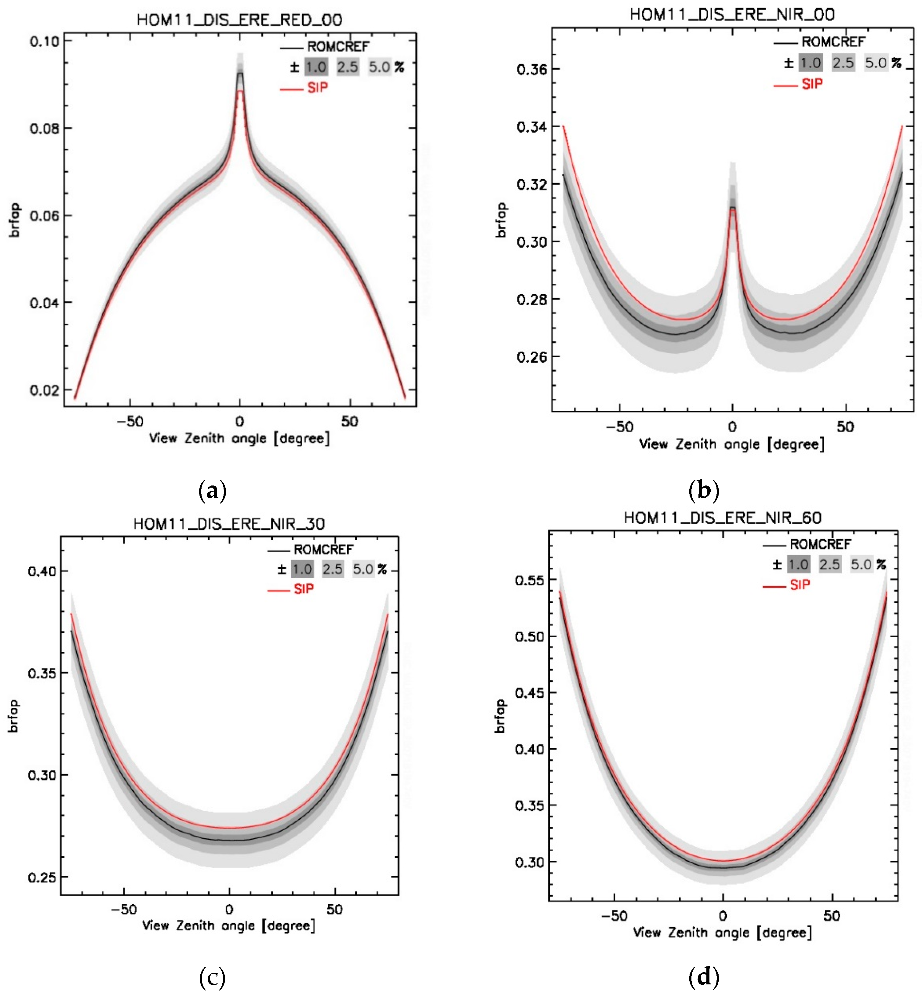
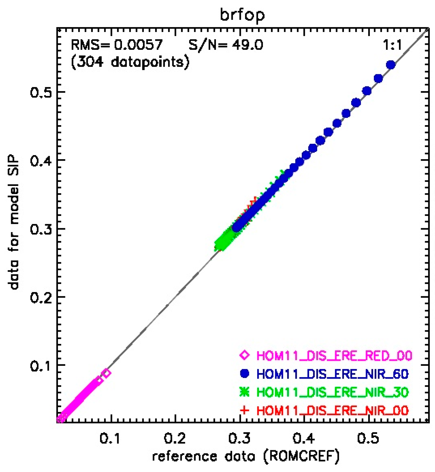
4.1. Evaluation in the RAMI Platform in Angular Space

The evaluation of the SIP model the by the RAMI platform is shown in Figure 2. The simulations of the SIP model at red and NIR bands agreed well with the reference “surrogate truth” by the RAMI On-line Model Checker (ROMC) reference dataset (ROMCREF). The simulation error of SIP at red and NIR bands can be within the $\pm$5.0% bias region, and most of the simulation errors were within the $\pm$2.5% bias region. The scatter plot is shown in Figure 3, which suggests the simulations of the SIP model closely followed the 1:1 line. The root-mean-square (RMS) error of the SIP model was 0.0057, which was less than 0.01. The signal-to-noise ratio (S/R) of the SIP model was 49.0, which was significantly larger than 1. There was a slight underestimation of BRF in the red band and a slight overestimation in the NIR band away from the hot spot direction, while this was more accurate at the hot spot direction, which might be due to the effect of the hot spot function. This can be affected by the leaf size, leaf shape and numerical singularities in the calculation. The hot spot effect has been considered in the first order scattering in both the red and NIR bands. In total, the evaluation results by the RAMI platform show that the high accuracy of the SIP model can meet the accuracy requirement of the BRF simulations in the angular space, especially at the hot spot direction.

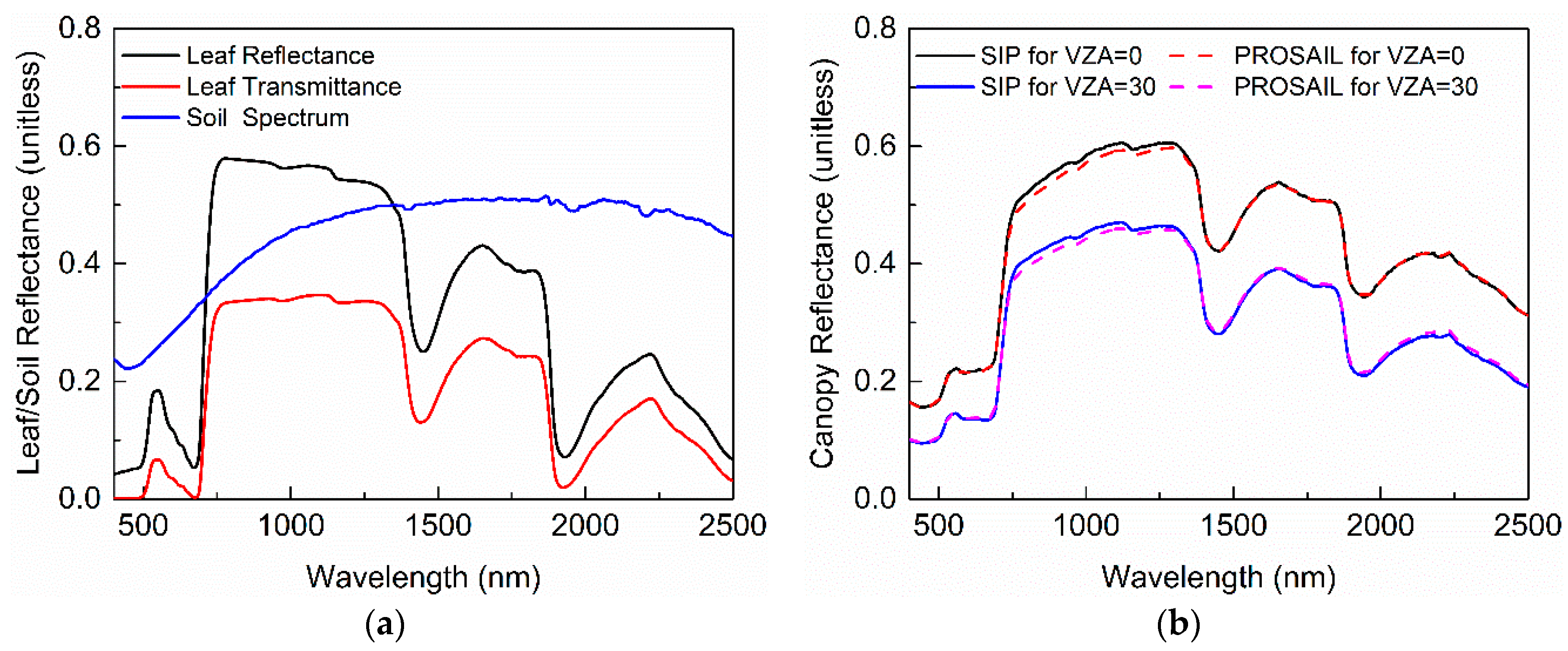
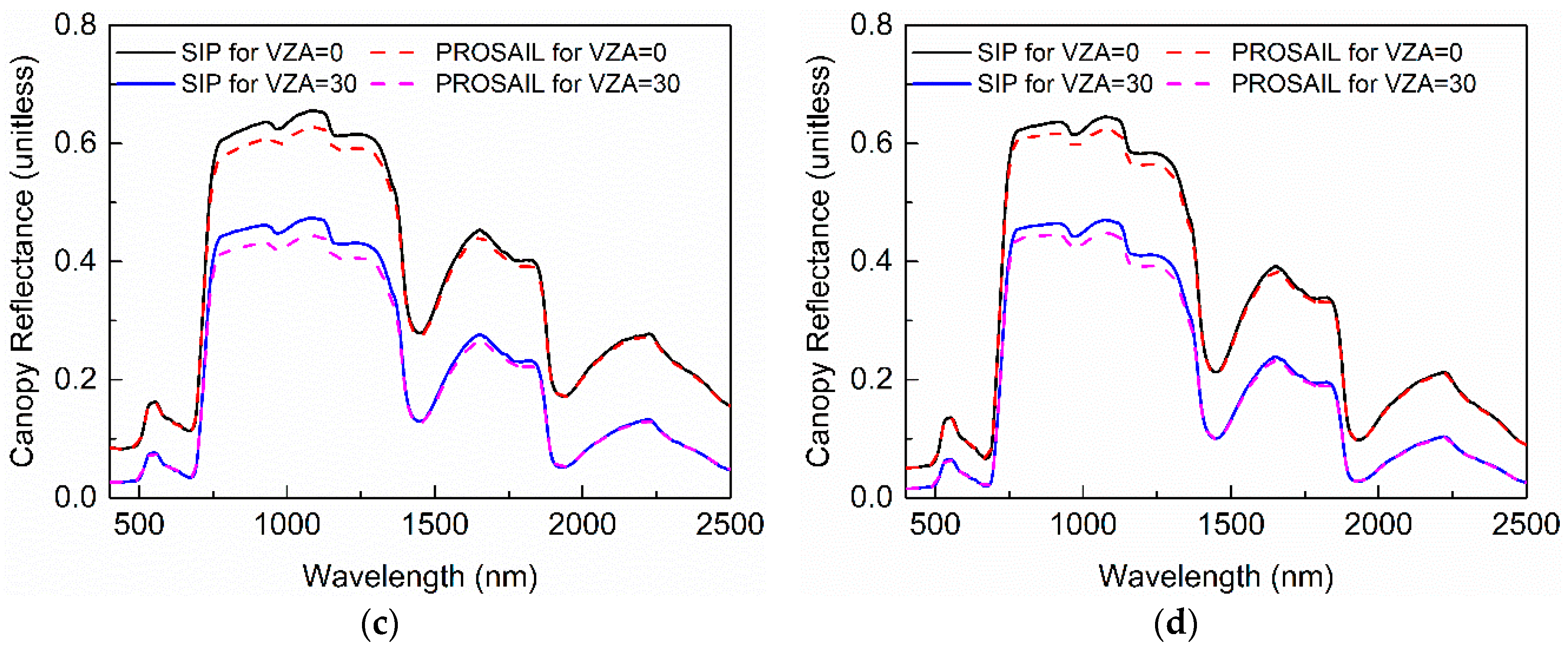
4.2. Evaluation by the PROSAIL Model in Hyperspectral Space

The evaluation of the SIP model by the PROSAIL model in hyperspectral space is shown in Figure 4. The simulations by SIP agreed well with that by PROSAIL across all the wavelengths from 400 nm–2500 nm. The valley in the red band at the canopy scale (Figure 4b) was not as significant as the leaf scale (Figure 4a), which was due to the soil background contribution at low LAI (LAI = 1). The canopy scale simulations by SIP were more accurate at low leaf reflectance (red) than at high leaf reflectance (NIR), which means there was smaller uncertainties in the single scattering calculations by SIP, compared with the multiple scattering calculations. In total, the evaluation result by the PROSAIL model shows the high accuracy of the SIP model when the LAI was 1, 3 and 5, respectively.

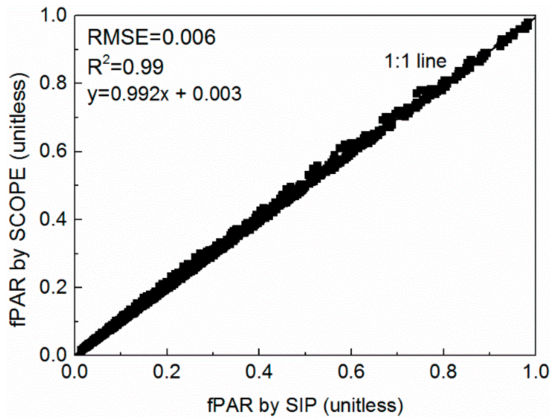
4.3. Evaluation the fPAR by the SCOPE Model

The fPAR estimation by SIP at different canopy structures (e.g., FVC, LAI and LAD), solar angles, and soil backgrounds was evaluated by the widely-used SCOPE model (Figure 5). The fPAR estimated by SIP agreed well with the estimations by SCOPE, and they were almost on the 1:1 line. The R² was 0.99, and the RMSE was 0.006, which show the high accuracy of the fPAR estimation by SIP. It is also obvious that there was no systematic error on the fPAR estimation by SIP. This was in accordance with the high accuracy of the BRF simulation in red band in Figure 2.

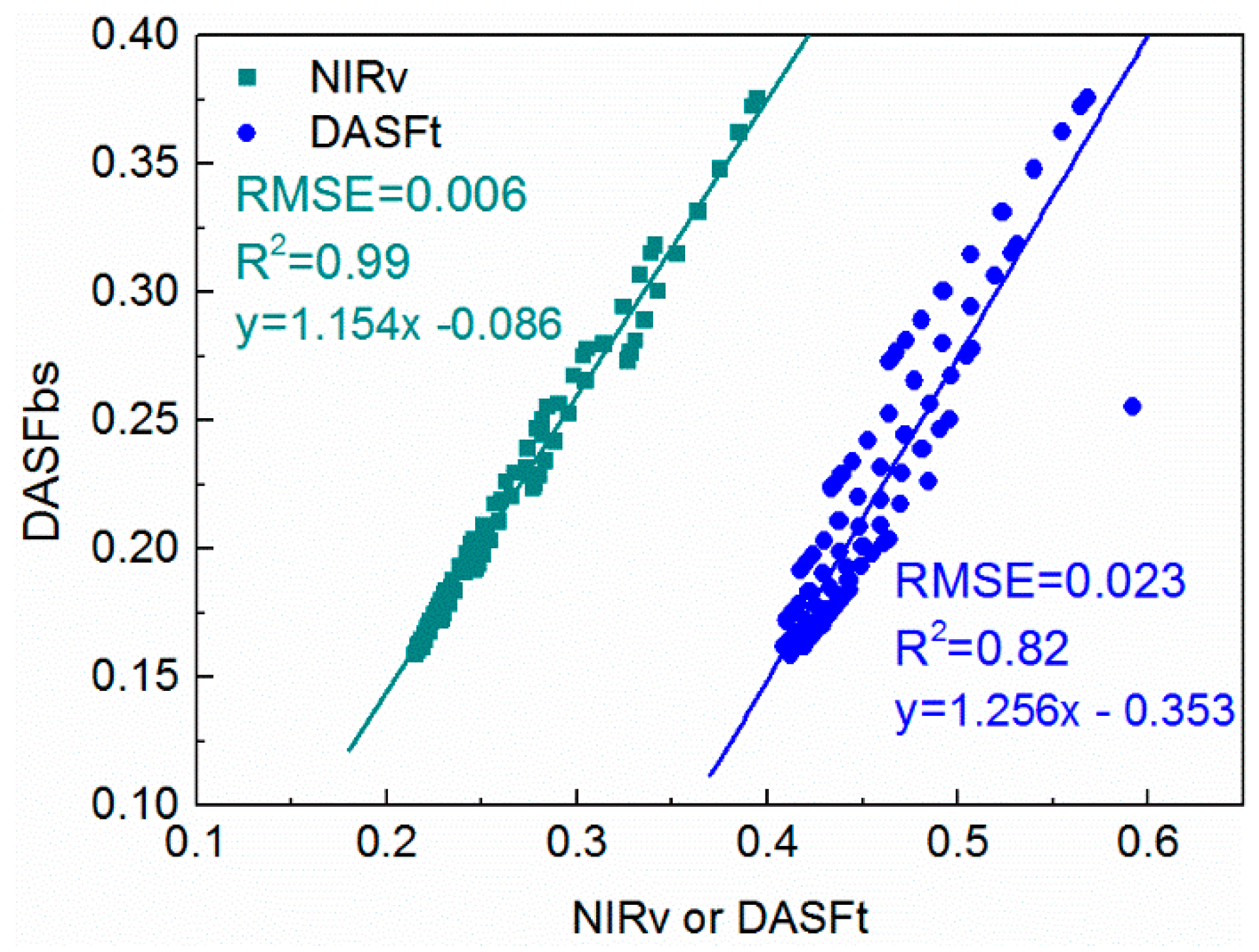
4.4. Impact of Soil Effect on DASF Calculation

Figure 6 shows the polar map of NIRv and DASF calculated directly from the total BRF of the soil-canopy system (DASF_t), and DASF calculated after the removal of the soil contribution as the black soil condition (DASF_bs). The corresponding scatter plots are shown in Figure 7. Figure 6 suggests the hot spot directions were more easily influenced by the soil due to the larger sunlit soil contribution. In the angular space, NIRv had a similar shape to DASF_bs, while DASF_t shows a different trend, especially the obvious high values around the hot spot directions. In Figure 7, NIRv was more linearly related with DASF_bs, with an R² of 0.99 and RMSE of 0.006, while DASF_t had a worse relationship with DASF_bs, with an R² of 0.82 and RMSE of 0.023. It is obvious to see the outlier for DASF_t at the hot spot direction in Figure 7. This suggests the simple index NIRv was promising as a good linear approximation of the important canopy structure parameter DASF_bs, without the use of a full radiative transfer model to eliminate the soil contribution.

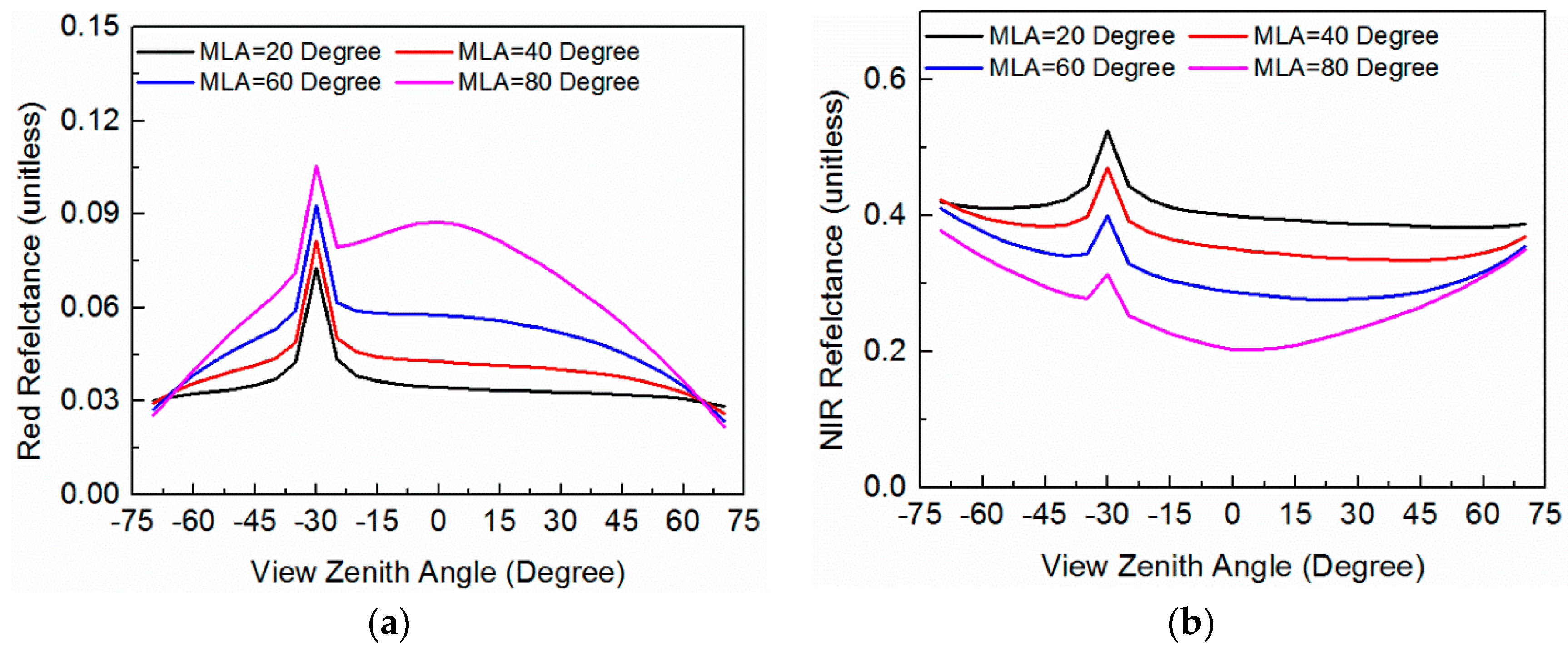
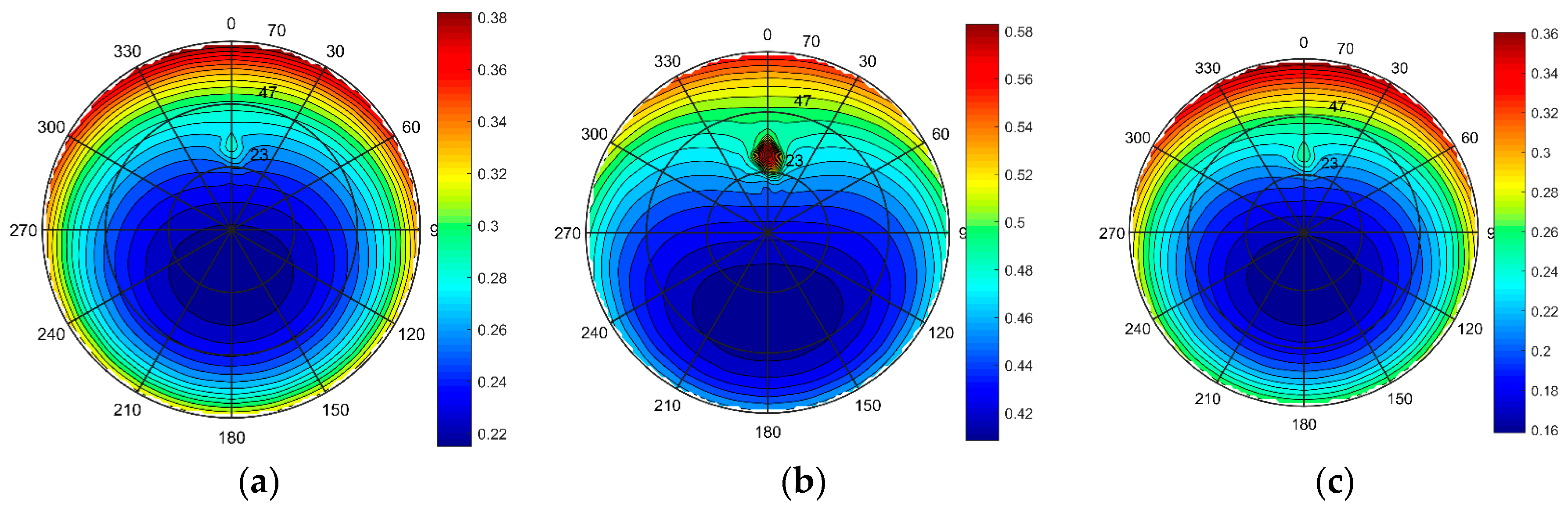
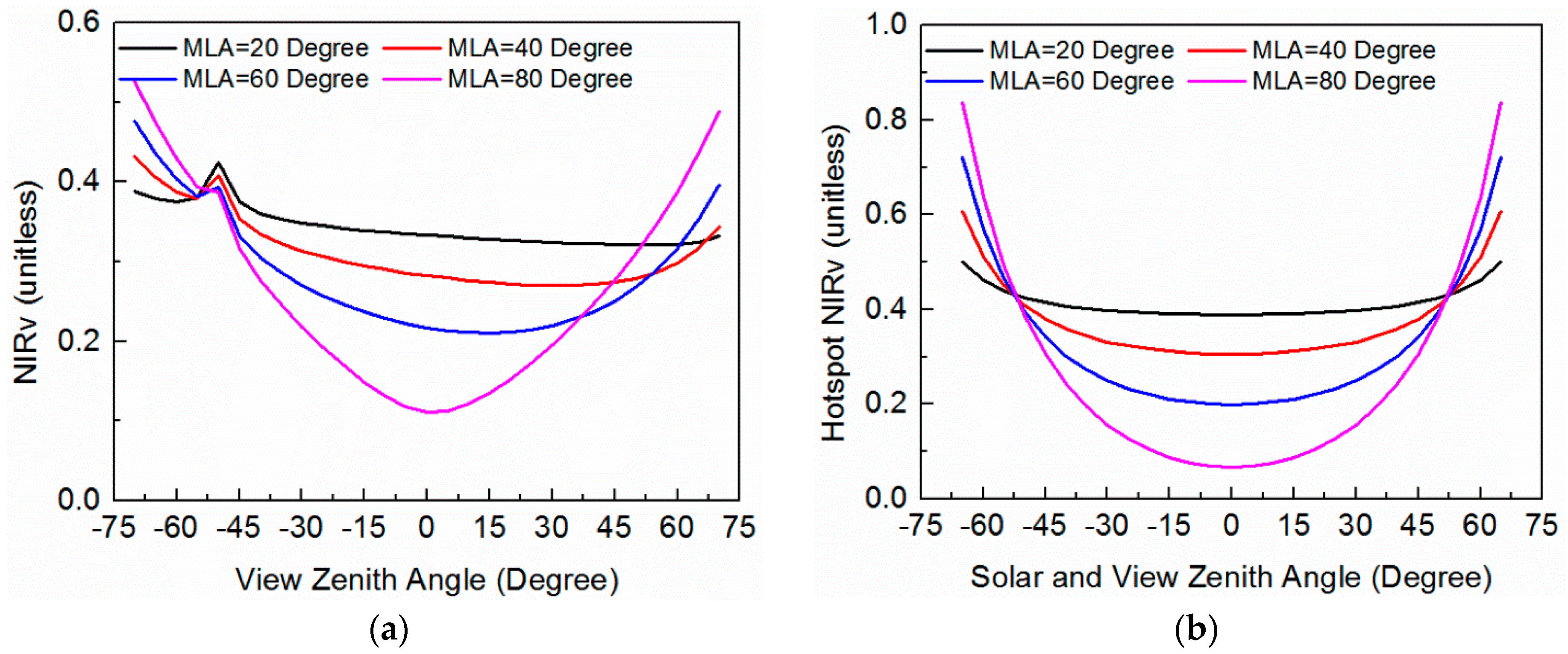
4.5. Impact of the Mean Leaf Inclination Angle on BRF and NIRv

The impact of LAD on BRF has been evaluated by SIP at different mean leaf inclination angles (MLA) by the ellipsoidal distribution function adopted in the PROSAIL model [10]. Figure 8 suggests that, even when the other parameters were the same as, e.g., LAI, only the difference in LAD can lead to significant BRF variations in both the red band and NIR band. This also suggests it was important to have the LAD information in biophysical parameter estimations, or a large inversion error may be introduced.

Figure 9 shows the NIRv angular variation in the principal plane when the solar zenith angle was 50° and in the hot spot direction. This suggests a different LAD can lead to different NIRv angular variation, especially for the hot spot NIRv. The more erect the leaves are, the larger the angular variation of hot spot NIRv. It is interesting to find that all the NIRv curves converged when the view zenith angle was about 57° (Figure 9b), and this is because at 57° the leaf projection G-function gives almost the same values regardless of the leaf inclination angle. This also suggests theoretically that, by using only two angular NIRv measurements (one was at 57° view zenith angle), it would be possible to extract the mean leaf inclination angle. Of course, more angular samplings of NIRv at the hot spot direction would be possible to achieve more robust mean leaf inclination angle estimations.

5. Discussion

The SIP model proposed in this study separates the first-order escape probability by the bidirectional gap fraction, which keeps the simplicity of the spectral invariant, and meanwhile explicitly describes the clumping effects and the leaf angle distribution. The SIP model shows high accuracy of BRF in the angular space and spectral space. The simplicity and high accuracy show that it is promising for application in future reflection-based biophysical variable estimations.

The SIP model is especially accurate at the hotspot direction, which has potential for biophysical variable estimation with the newly launched DSCOVR EPIC [16]. At the hot spot direction, the bidirectional gap fraction $P_{so}$ in Equation (4) would be reduced to the directional gap fraction $P_s$ or $P_o$ because the $P_o·C_{HS}$ or $P_s·C_{HS}$ is equal to 1. This greatly simplifies the radiative transfer process, and would largely reduce the uncertainties in the hot spot correction function $C_{HS}$ in Equation (4). The angular distribution of NIRv especially in the hot spot directions shows the sensitivity of NIRv to the mean leaf inclination angle (Figure 9), which suggests that it is promising for estimating the mean leaf inclination angle by NIRv from multi-angular EPIC observations and the proposed SIP model. Usually, the effects of the leaf inclination angle and multi-angular clumping index are coupled, while their retrievals can still be constrained by their angular features, e.g., the NIRv would converge when the view zenith angle was about 57° for any leaf inclination angle (Figure 9), and the results of Kucharik et al. [32] show that the clumping index with a zenith angle between 20°–60° obeys an exponential or even linear function. Due to the sub-hourly high temporal frequency, the EPIC can almost always acquire two observations with a solar-sensor zenith angle of about 57° each day, which shows the feasibility of retrievals.

Besides this, the estimation of biophysical variables requires the elimination of the soil background contribution. The simple vegetation index, NIRv, was shown to give a good linear approximation of the canopy structure parameter DASF (Figure 7) and was not influenced much by the soil background effect (Figure 6). Thus, it is worth trying NIRv for the cost function of biophysical variable retrievals, in contrast to the independent use of the red and NIR band in the look-up-table [17]. By using NIRv, we do not need to account for the single scattering contribution of the soil ($BR{F}_S$ in Equation (7)) and the photon interactions between vegetation and soil ($BR{F}_M$ in Equation (8)), and thus we only need to calculate the $BR{F}_V$ in Equation (1), which would further simplify the radiative transfer process. The high accuracy of the proposed SIP model across the whole wavelength (400 nm–2500 nm) in Figure 4 also shows it would be promising to retrieve the canopy structure and leaf optics at the same time by the joint use of hyperspectral and multi-angular observations. To improve the retrieval accuracy, the recent progress in the field of RT forwarding modeling, inversion and validation should be accounted for, such as the mixed pixel effect [40,41], the variation of the vegetation density [42,43,44], the topography effect [45,46,47,48], and the spatial–temporal constraints [49,50,51].

6. Conclusions

We develop a simple radiative transfer model based on spectral invariant properties (SIP). The SIP model adopts the method of calculate the single scattering contribution from the PROSAIL model, but explicitly describes the clumping effects and the leaf angle distribution. The multiple scattering within the canopy, and the interactions between the canopy and the soil, are calculated in the framework of the spectral invariant, which has the advantage of simplicity compared with the SOSA method [21].The SIP model agreed well with the reference values on BRF and fPAR from the RAMI platform, the PROSAIL model and the SCOPE model, with an R² of 0.99 and an RMSE of 0.006. We also found that NIRv gave a good linear approximation of the canopy structure parameter, DASF. NIRv was robust to the soil background contribution, but was sensitive to the leaf inclination angle. Results suggest NIRv is a promising index for future biophysical variable estimations by the proposed SIP model, especially for the joint use of the hyperspectral and multi-angular observations.

References

1. Zhao, J.; Li, J.; Liu, Q.; Fan, W.; Zhong, B.; Wu, S.; Yang, L.; Zeng, Y.; Xu, B.; Yin, G. Leaf Area Index Retrieval Combining HJ1/CCD and Landsat8/OLI Data in the Heihe River Basin, China. Remote Sens. 2015, 7, 6862–6885. [Google Scholar] [CrossRef] [Green Version]
2. Yin, G.; Li, A.; Jin, H.; Zhao, W.; Bian, J.; Qu, Y.; Zeng, Y.; Xu, B. Derivation of temporally continuous LAI reference maps through combining the LAINet observation system with CACAO. Agric. For. Meteorol. 2017, 233, 209–221. [Google Scholar] [CrossRef]
3. Mu, X.; Hu, R.; Zeng, Y.; McVicar, T.R.; Ren, H.; Song, W.; Wang, Y.; Casa, R.; Qi, J.; Xie, D. Estimating structural parameters of agricultural crops from ground-based multi-angular digital images with a fractional model of sun and shade components. Agric. For. Meteorol. 2017, 246, 162–177. [Google Scholar] [CrossRef]
4. Yan, K.; Park, T.; Chen, C.; Xu, B.; Song, W.; Yang, B.; Zeng, Y.; Liu, Z.; Yan, G.; Knyazikhin, Y. Generating Global Products of LAI and FPAR From SNPP-VIIRS Data: Theoretical Background and Implementation. IEEE Trans. Geosci. Remote Sens. 2018, 56, 2119–2137. [Google Scholar] [CrossRef]
5. Xu, B.; Park, T.; Yan, K.; Chen, C.; Zeng, Y.; Song, W.; Yin, G.; Li, J.; Liu, Q.; Knyazikhin, Y. Analysis of Global LAI/FPAR Products from VIIRS and MODIS Sensors for Spatio-Temporal Consistency and Uncertainty from 2012–2016. Forests 2018, 9, 73. [Google Scholar] [CrossRef]
6. Yin, G.; Li, J.; Liu, Q.; Fan, W.; Xu, B.; Zeng, Y.; Zhao, J. Regional Leaf Area Index Retrieval Based on Remote Sensing: The Role of Radiative Transfer Model Selection. Remote Sens. 2015, 7, 4604–4625. [Google Scholar] [CrossRef] [Green Version]
7. Yin, G.; Li, J.; Liu, Q.; Li, L.; Zeng, Y.; Xu, B.; Yang, L.; Zhao, J. Improving Leaf Area Index Retrieval over Heterogeneous Surface by Integrating Textural and Contextual Information: A Case Study in the Heihe River Basin. IEEE Geosci. Remote Sens. Lett. 2015, 12, 359–363. [Google Scholar]
8. Zeng, Y.; Li, J.; Liu, Q.; Hu, R.; Mu, X.; Fan, W.; Xu, B.; Yin, G.; Wu, S. Extracting Leaf Area Index by Sunlit Foliage Component from Downward-Looking Digital Photography under Clear-Sky Conditions. Remote Sens. 2015, 7, 13410–13435. [Google Scholar] [CrossRef] [Green Version]
9. Kuusk, A. A two-layer canopy reflectance model. J. Quant. Spectrosc. Radiat. Transf. 2001, 71, 1–9. [Google Scholar] [CrossRef]
10. Verhoef, W. Light scattering by leaf layers with application to canopy reflectance modeling: The SAIL model. Remote Sens. Environ. 1984, 16, 125–141. [Google Scholar] [CrossRef] [Green Version]
11. Kuusk, A.; Nilson, T. A directional multispectral forest reflectance model. Remote Sens. Environ. 2000, 72, 244–252. [Google Scholar] [CrossRef]
12. Chen, J.M.; Leblanc, S.G. A four-scale bidirectional reflectance model based on canopy architecture. IEEE Trans. Geosci. Remote Sens. 1997, 35, 1316–1337. [Google Scholar] [CrossRef] [Green Version]
13. Huang, D.; Knyazikhin, Y.; Wang, W.; Deering, D.W.; Stenberg, P.; Shabanov, N.; Tan, B.; Myneni, R.B. Stochastic transport theory for investigating the three-dimensional canopy structure from space measurements. Remote Sens. Environ. 2008, 112, 35–50. [Google Scholar] [CrossRef]
14. Zeng, Y.; Li, J.; Liu, Q.; Yin, G.; Xu, B.; Fan, W.; Zhao, J. A canopy radiative transfer model suitable for heterogeneous Agro-Forestry scenes. In Proceedings of the IEEE International of Geoscience and Remote Sensing Symposium (IGARSS), Beijing, China, 10–15 July 2016; pp. 3648–3651. [Google Scholar]
15. Zeng, Y.; Li, J.; Liu, Q.; Huete, A.R.; Yin, G.; Xu, B.; Fan, W.; Zhao, J.; Yan, K.; Mu, X. A Radiative Transfer Model for Heterogeneous Agro-Forestry Scenarios. IEEE Trans. Geosci. Remote Sens. 2016, 54, 4613–4628. [Google Scholar] [CrossRef]
16. Marshak, A.; Knyazikhin, Y. The spectral invariant approximation within canopy radiative transfer to support the use of the EPIC/DSCOVR oxygen B-band for monitoring vegetation. J. Quant. Spectrosc. Radiat. Transf. 2017, 191, 7–12. [Google Scholar] [CrossRef] [PubMed] [Green Version]
17. Knyazikhin, Y.; Martonchik, J.; Myneni, R.B.; Diner, D.; Running, S.W. Synergistic algorithm for estimating vegetation canopy leaf area index and fraction of absorbed photosynthetically active radiation from MODIS and MISR data. J. Geophys. Res. Atmos. 1998, 103, 32257–32275. [Google Scholar] [CrossRef] [Green Version]
18. Knyazikhin, Y.; Schull, M.A.; Stenberg, P.; Mõttus, M.; Rautiainen, M.; Yang, Y.; Marshak, A.; Carmona, P.L.; Kaufmann, R.K.; Lewis, P. Hyperspectral remote sensing of foliar nitrogen content. Proc. Natl. Acad. Sci. USA 2013, 110, E185–E192. [Google Scholar] [CrossRef] [PubMed]
19. Stenberg, P.; Mõttus, M.; Rautiainen, M. Photon recollision probability in modelling the radiation regime of canopies—A review. Remote Sens. Environ. 2016, 183, 98–108. [Google Scholar] [CrossRef]
20. Huang, D.; Knyazikhin, Y.; Dickinson, R.E.; Rautiainen, M.; Stenberg, P.; Disney, M.; Lewis, P.; Cescatti, A.; Tian, Y.; Verhoef, W. Canopy spectral invariants for remote sensing and model applications. Remote Sens. Environ. 2007, 106, 106–122. [Google Scholar] [CrossRef] [Green Version]
21. Myneni, R.; Asrar, G.; Kanemasu, E. Light scattering in plant canopies: The method of successive orders of scattering approximations (SOSA). Agric. For. Meteorol. 1987, 39, 1–12. [Google Scholar] [CrossRef]
22. Stenberg, P.; Lukeš, P.; Rautiainen, M.; Manninen, T. A new approach for simulating forest albedo based on spectral invariants. Remote Sens. Environ. 2013, 137, 12–16. [Google Scholar] [CrossRef]
23. Majasalmi, T.; Rautiainen, M.; Stenberg, P. Modeled and measured fPAR in a boreal forest: Validation and application of a new model. Agric. For. Meteorol. 2014, 189, 118–124. [Google Scholar] [CrossRef]
24. Yang, B.; Knyazikhin, Y.; Mõttus, M.; Rautiainen, M.; Stenberg, P.; Yan, L.; Chen, C.; Yan, K.; Choi, S.; Park, T. Estimation of leaf area index and its sunlit portion from DSCOVR EPIC data: Theoretical basis. Remote Sens. Environ. 2017, 198, 69–84. [Google Scholar] [CrossRef] [PubMed] [Green Version]
25. Chen, J.M. Optically-based methods for measuring seasonal variation of leaf area index in boreal conifer stands. Agric. For. Meteorol. 1996, 80, 135–163. [Google Scholar] [CrossRef]
26. Mõttus, M. Photon recollision probability in discrete crown canopies. Remote Sens. Environ. 2007, 110, 176–185. [Google Scholar] [CrossRef]
27. Stenberg, P. Simple analytical formula for calculating average photon recollision probability in vegetation canopies. Remote Sens. Environ. 2007, 109, 221–224. [Google Scholar] [CrossRef]
28. Pisek, J.; Sonnentag, O.; Richardson, A.D.; Mõttus, M. Is the spherical leaf inclination angle distribution a valid assumption for temperate and boreal broadleaf tree species? Agric. For. Meteorol. 2013, 169, 186–194. [Google Scholar] [CrossRef]
29. Chen, J.M.; Menges, C.H.; Leblanc, S.G. Global mapping of foliage clumping index using multi-angular satellite data. Remote Sens. Environ. 2005, 97, 447–457. [Google Scholar] [CrossRef]
30. Ryu, Y.; Sonnentag, O.; Nilson, T.; Vargas, R.; Kobayashi, H.; Wenk, R.; Baldocchi, D.D. How to quantify tree leaf area index in an open savanna ecosystem: A multi-instrument and multi-model approach. Agric. For. Meteorol. 2010, 150, 63–76. [Google Scholar] [CrossRef]
31. Fang, H.; Liu, W.; Li, W.; Wei, S. Estimation of the directional and whole apparent clumping index (ACI) from indirect optical measurements. ISPRS J. Photogramm. Remote Sens. 2018, 144, 1–13. [Google Scholar] [CrossRef]
32. Kucharik, C.J.; Norman, J.M.; Gower, S.T. Characterization of radiation regimes in nonrandom forest canopies: Theory, measurements, and a simplified modeling approach. Tree Physiol. 1999, 19, 695–706. [Google Scholar] [CrossRef] [PubMed]
33. Marshak, A. The effect of the hot spot on the transport equation in plant canopies. J. Quant. Spectrosc. Radiat. Transf. 1989, 42, 615–630. [Google Scholar] [CrossRef]
34. Rautiainen, M.; Stenberg, P. Application of photon recollision probability in coniferous canopy reflectance simulations. Remote Sens. Environ. 2005, 96, 98–107. [Google Scholar] [CrossRef]
35. Widlowski, J.-L.; Robustelli, M.; Disney, M.; Gastellu-Etchegorry, J.-P.; Lavergne, T.; Lewis, P.; North, P.; Pinty, B.; Thompson, R.; Verstraete, M. The RAMI On-line Model Checker (ROMC): A web-based benchmarking facility for canopy reflectance models. Remote Sens. Environ. 2008, 112, 1144–1150. [Google Scholar] [CrossRef] [Green Version]
36. Schull, M.A.; Knyazikhin, Y.; Xu, L.; Samanta, A.; Carmona, P.L.; Lepine, L.; Jenkins, J.; Ganguly, S.; Myneni, R.B. Canopy spectral invariants, Part 2: Application to classification of forest types from hyperspectral data. J. Quant. Spectrosc. Radiat. Transf. 2011, 112, 736–750. [Google Scholar] [CrossRef] [Green Version]
37. Badgley, G.; Field, C.B.; Berry, J.A. Canopy near-infrared reflectance and terrestrial photosynthesis. Sci. Adv. 2017, 3, e1602244. [Google Scholar] [CrossRef] [PubMed] [Green Version]
38. Van der Tol, C.; Verhoef, W.; Timmermans, J.; Verhoef, A.; Su, Z. An integrated model of soil-canopy spectral radiances, photosynthesis, fluorescence, temperature and energy balance. Biogeosciences 2009, 6, 3109–3129. [Google Scholar] [CrossRef] [Green Version]
39. Widlowski, J.L.; Mio, C.; Disney, M.; Adams, J.; Andredakis, I.; Atzberger, C.; Brennan, J.; Busetto, L.; Chelle, M.; Ceccherini, G.; et al. The fourth phase of the radiative transfer model intercomparison (RAMI) exercise: Actual canopy scenarios and conformity testing. Remote Sens. Environ. 2015, 169, 418–437. [Google Scholar] [CrossRef] [Green Version]
40. Zeng, Y.; Li, J.; Liu, Q.; Li, L.; Xu, B.; Yin, G.; Peng, J. A sampling strategy for remotely sensed LAI product validation over heterogeneous land surfaces. IEEE J. Sel. Top. Appl. Earth Obs. Remote Sens. 2014, 7, 3128–3142. [Google Scholar] [CrossRef]
41. Yu, W.; Li, J.; Liu, Q.; Zeng, Y.; Zhao, J.; Xu, B.; Yin, G. Global Land Cover Heterogeneity Characteristics at Moderate Resolution for Mixed Pixel Modeling and Inversion. Remote Sens. 2018, 10, 856. [Google Scholar] [CrossRef]
42. Xu, B.; Li, J.; Liu, Q.; Huete, A.R.; Yu, Q.; Zeng, Y.; Yin, G.; Zhao, J.; Yang, L. Evaluating Spatial Representativeness of Station Observations for Remotely Sensed Leaf Area Index Products. IEEE J. Sel. Top. Appl. Earth Obs. Remote Sens. 2016, 9, 3267–3282. [Google Scholar] [CrossRef]
43. Xu, B.; Li, J.; Liu, Q.; Zeng, Y.; Yin, G.; Fan, W.; Zhao, J. A method for spatial upscaling of ground LAI measurements to the remotely sensed product pixel grid. In Proceedings of the IEEE International Geoscience and Remote Sensing Symposium (IGARSS), Beijing, China, 10–15 July 2016; pp. 3528–3531. [Google Scholar]
44. Dou, B.; Wen, J.; Li, X.; Liu, Q.; Peng, J.; Xiao, Q.; Zhang, Z.; Tang, Y.; Wu, X.; Lin, X. Wireless sensor network of typical land surface parameters and its preliminary applications for coarse-resolution remote sensing pixel. Int. J. Distrib. Sens. Netw. 2016, 12, 9639021. [Google Scholar] [CrossRef]
45. Yin, G.; Li, A.; Wu, S.; Fan, W.; Zeng, Y.; Yan, K.; Xu, B.; Li, J.; Liu, Q. PLC: A simple and semi-physical topographic correction method for vegetation canopies based on path length correction. Remote Sens. Environ. 2018, 215, 184–198. [Google Scholar] [CrossRef]
46. Fan, W.; Li, J.; Liu, Q.; Zhang, Q.; Yin, G.; Li, A.; Zeng, Y.; Xu, B.; Xu, X.; Zhou, G. Topographic Correction of Forest Image Data Based on the Canopy Reflectance Model for Sloping Terrains in Multiple Forward Mode. Remote Sens. 2018, 10, 717. [Google Scholar] [CrossRef]
47. Yan, G.; Tong, Y.; Yan, K.; Mu, X.; Chu, Q.; Zhou, Y.; Liu, Y.; Qi, J.; Li, L.; Zeng, Y. Temporal Extrapolation of Daily Downward Shortwave Radiation Over Cloud-Free Rugged Terrains. Part 1: Analysis of Topographic Effects. IEEE Trans. Geosci. Remote Sens. 2018, PP, 1–20. [Google Scholar] [CrossRef]
48. Yin, G.; Li, A.; Zeng, Y.; Xu, B.; Zhao, W.; Nan, X.; Jin, H.; Bian, J. A cost-constrained sampling strategy in support of LAI product validation in mountainous areas. Remote Sens. 2016, 8, 704. [Google Scholar] [CrossRef]
49. Zeng, Y.; Li, J.; Liu, Q.; Qu, Y.; Huete, A.R.; Xu, B.; Yin, G.; Zhao, J. An Optimal Sampling Design for Observing and Validating Long-Term Leaf Area Index with Temporal Variations in Spatial Heterogeneities. Remote Sens. 2015, 7, 1300–1319. [Google Scholar] [CrossRef] [Green Version]
50. Zeng, Y.; Li, J.; Liu, Q.; Huete, A.R.; Xu, B.; Yin, G.; Zhao, J.; Yang, L.; Fan, W.; Wu, S. An Iterative BRDF/NDVI Inversion Algorithm Based on A Posteriori Variance Estimation of Observation Errors. IEEE Trans. Geosci. Remote Sens. 2016, 54, 6481–6496. [Google Scholar] [CrossRef]
51. Xu, B.; Li, J.; Park, T.; Liu, Q.; Zeng, Y.; Yin, G.; Zhao, J.; Fan, W.; Yang, L.; Knyazikhin, Y. An integrated method for validating long-term leaf area index products using global networks of site-based measurements. Remote Sens. Environ. 2018, 209, 134–151. [Google Scholar] [CrossRef]
Figure 1. The framework of the spectral invariant properties (SIP) model on how to describe the radiative transfer process from spectral invariants, which are derived bfromcanopy structure parameters. Detailed descriptions of each item are in Section 2.
Remotesensing 10 01508 g001
Figure 2. The bidirectional reflectance factor (BRF) of the SIP model in the red (a) and near infra-red (NIR) bands with the solar zenith angle at 0° (b), 30° (c), 60° (d) in the orthogonal plane evaluated by the RAMI On-line Model Checker (ROMC) reference dataset (ROMCREF). “HOM11” is the number of the standard RAMI scene, “DIS” represents the discrete medium of the leaves, “ERE” represents the erectophile leaf angle distribution (LAD) type, and “OP” means the orthogonal plane.
Remotesensing 10 01508 g002
Figure 3. The scatter plots between the BRF of the SIP simulations and the RAMI reference values (ROMCREF) in the red and NIR bands in the orthogonal plane at the RAMI platform in Figure 2. The root mean square (RMS) error and signal-to-noise (S/N) were directly calculated with the RAMI platform (http://romc.jrc.ec.europa.eu/).
Remotesensing 10 01508 g003
Figure 4. The input leaf/soil spectrum (a) and canopy-scale spectrum simulations by SIP and PROSAIL (bd). VZA represents the view zenith angle. The leaf area index (LAI) is 1 (b), 3 (c) or 5 (d), respectively, LAD is erectophile, and the solar zenith angle is 0°. The other input parameters are the same as Table 1.
Remotesensing 10 01508 g004aRemotesensing 10 01508 g004b
Figure 5. The evaluation of the SIP model by the widely-used SCOPE model at different canopy structures, solar angles, and soil backgrounds. The list of variables and their ranges are in Table 2.
Remotesensing 10 01508 g005
Figure 6. The polar map of NIRv, (a) the directional area scattering factor (DASF) calculated without the removal of the soil (b), and DASF calculated after the removal of the soil (c). The LAI is 1, LAD is erectophile, and the solar zenith angle is 30°. The other input parameters are the same as Table 1.
Remotesensing 10 01508 g006
Figure 7. The scatter plot between NIRv or DASF calculated from total scene BRF without the removal of the soil (DASFt), with DASF calculated at the black soil condition (DASFbs). The LAI is 1, and the solar zenith angle is 30°. The other input parameters are the same as Table 1 or Figure 5.
Remotesensing 10 01508 g007
Figure 8. The reflectance simulated by the SIP model in the red band (a) and NIR band (b) at different mean leaf inclination angles (MLA) in the principal plane. The LAI is 1, and the solar zenith angle is 30°. The other input parameters are the same as Table 1.
Remotesensing 10 01508 g008
Figure 9. The NIRv simulated by the SIP model when the solar zenith angle is 50° (a), and when the solar direction coincides with the view direction for hot spot observation (b). MLA represents the mean leaf inclination angle. The LAI is 1, and other input parameters are the same as Table 1.
Remotesensing 10 01508 g009