Calibrating the SAR SSH of Sentinel-3A and CryoSat-2 over the Corsica Facilities

 ,
, 
Abstract
:
1. Introduction
2. Data and Methodology
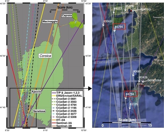
2.1. Data
Sentinel-3A:
- Data sources: S3-PDGS (payload data ground segment) reprocessing 2017, Non-Time Critical (NTC) products: cycle 5–19, processing baseline 2.15 [10]. The processing baseline (PB) 2.15 consists of the following processors: SRAL L1 IPF V6.11, MWR L1 IPF V6.04, SRAL L2 IPF V6.07.
- Sentinel-3A SRAL (Ku/C Radar Altimeter) processing for SAR and Pseudo LRM (PLRM) and applied corrections
- ○
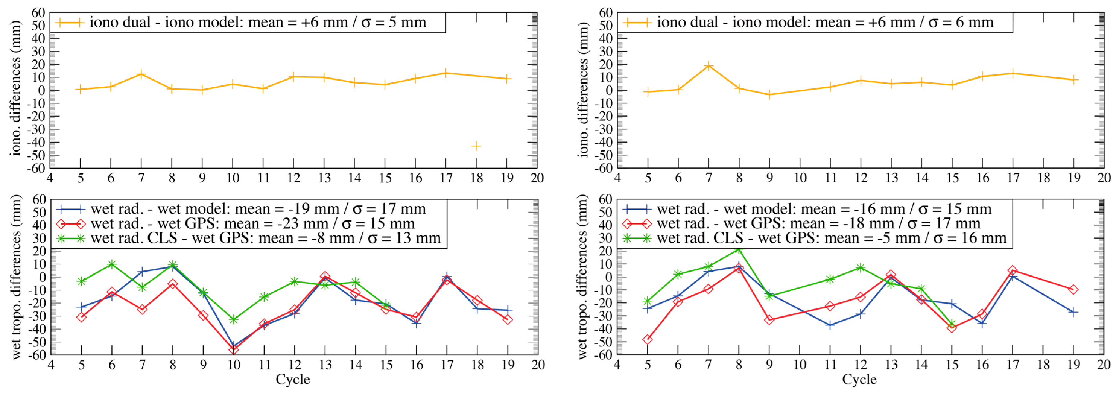
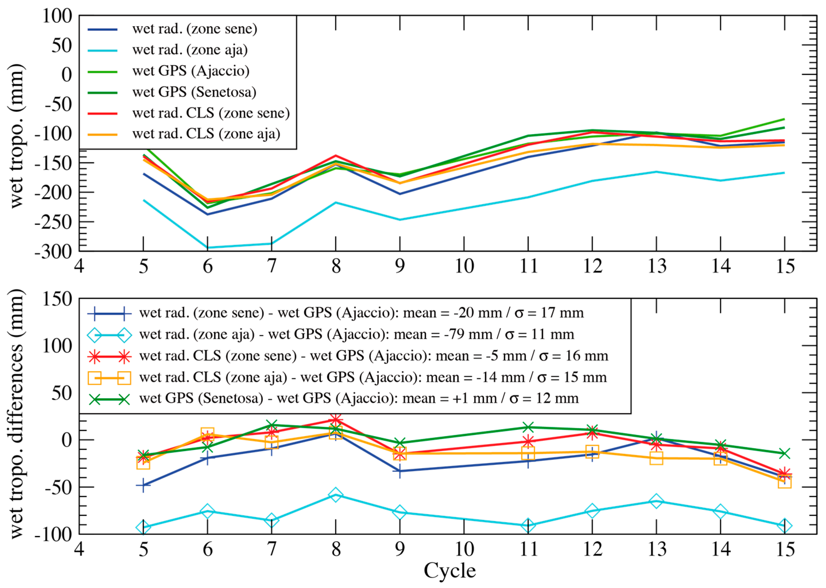
- Standard processing: dual-frequency ionosphere measurement and wet troposphere radiometry. In this study, we also compared the dual frequency ionosphere measurements with the global ionosphere maps model (GIM), together with a comparison of the wet troposphere radiometer measurements with the wet troposphere model from European Centre for Medium-Range Weather Forecasts (ECMWF)). The chosen wet correction for the model corresponds to the field that is computed at sea level (MOD_WET_TROPO_COR_ZERO_ALTITUDE)
- ○
- Dry troposphere
- ○
- Sea state bias (SSB)
- ○
- Solid, loading and pole tides
- In situ data
- ○
- Ajaccio: Service Hydrographique et Océanographique de la Marine (SHOM) radar tide gauge data in real time
- ○
- Senetosa: pressure tide gauges (data retrieved end of July 2017)
CryoSat-2:
- Data sources: from SARvatore service at ESA G-POD (https://gpod.eo.esa.int/services/CRYOSAT_SAR/) using baseline B products with two different retrackers. It is important to note that this product does not correspond to the current baseline C products processed by the CryoSat-2 payload data ground segment (PDGS), the main difference being the correction of a known range bias of 673 mm:
- ○
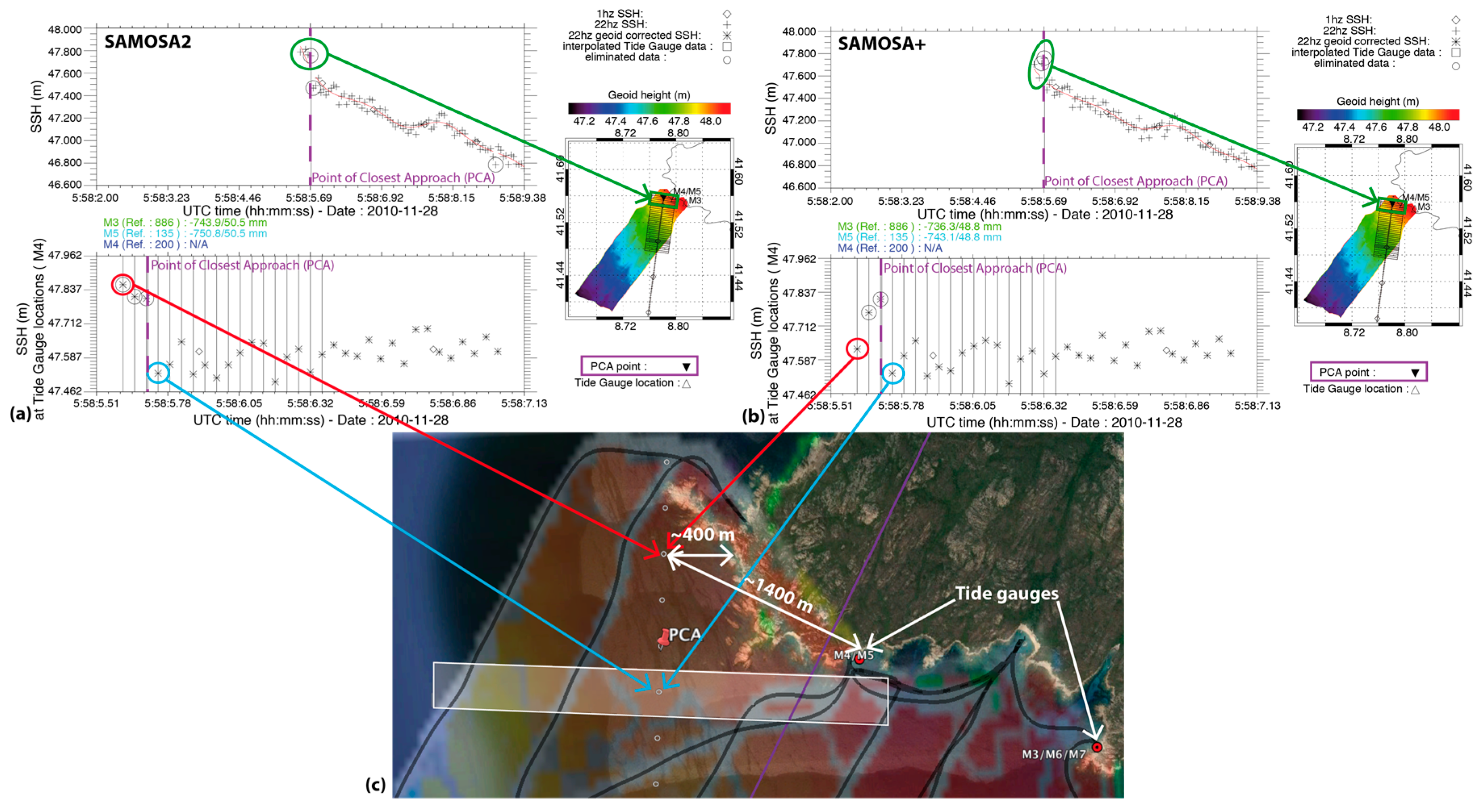
- SAMOSA2 retracker (default): The SAMOSA (SAR Altimetry MOde Studies and Applications) model [11] has been implemented in its first-order formulation (SAMOSA2) in a retracker as in [12]. This retracker uses a look-up table to mitigate the effect of the model’s approximation of the squared PTR (point target response) with a Gaussian curve, it implements a stack masking for the Doppler beams padded to zero and has in principle no enhancement in the coastal zone.
- ○
- SAMOSA+ retracker (the SAMOSA2 model tailored for inland water, sea ice and the coastal zone domain): in the case of SAMOSA+, the open ocean SAMOSA [11] model and retracker [13] has been implemented in the retracking scheme with two significant additions [12]: The first one concerns the selection of the first-guess epoch. This is not selected as the position of the waveform peak but as the position of the moving correlation peak in 20 consecutive waveforms (after aligning them for tracker shift). The rationale behind this choice is to attempt to mitigate the typical off-ranging effect in coastal data. The second concerns the treatment of land-contaminated waveforms. In case waveforms are not contaminated by land, the SAMOSA model was used with the mean square slope set to zero, i.e., as in [13], whereas in the case of land contaminated waveforms, we used a dual step retracking: in the first step, the SWH is still estimated as in [13], while in the second step, the SWH was set to zero and the third free parameter in the retracking becomes the mean square slope. The output of this second step is the range and the amplitude Pu (retracked waveform amplitude, see Equation (22) in [12]).
- Cryosat-2 SIRAL (synthetic aperture interferometric radar altimeter) data processing for SAR and applied corrections
- ○
- Dry troposphere
- ○
- Wet troposphere from ECMWF model
- ○
- Ionosphere from GIM
- ○
- Sea state bias = 3.5% of SWH
- ○
- Solid, loading and pole tides
- In situ data
- ○
- Ajaccio: SHOM radar tide gauge data in real time
- ○
- Senetosa: pressure tide gauges (data retrieved end of July 2017)
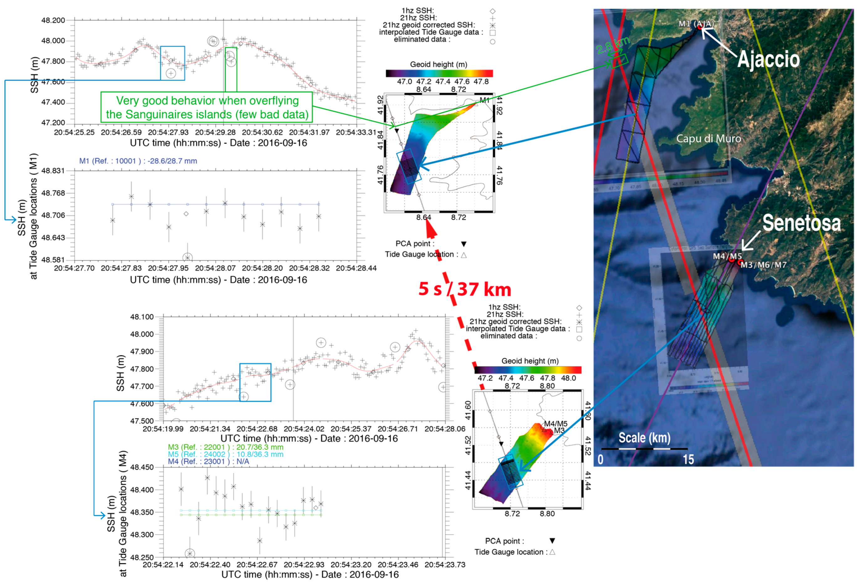
2.2. Methodology
3. Results
3.1. Solving the Vertical Offset in the Ajaccio Tide-Gauge-Derived SSH
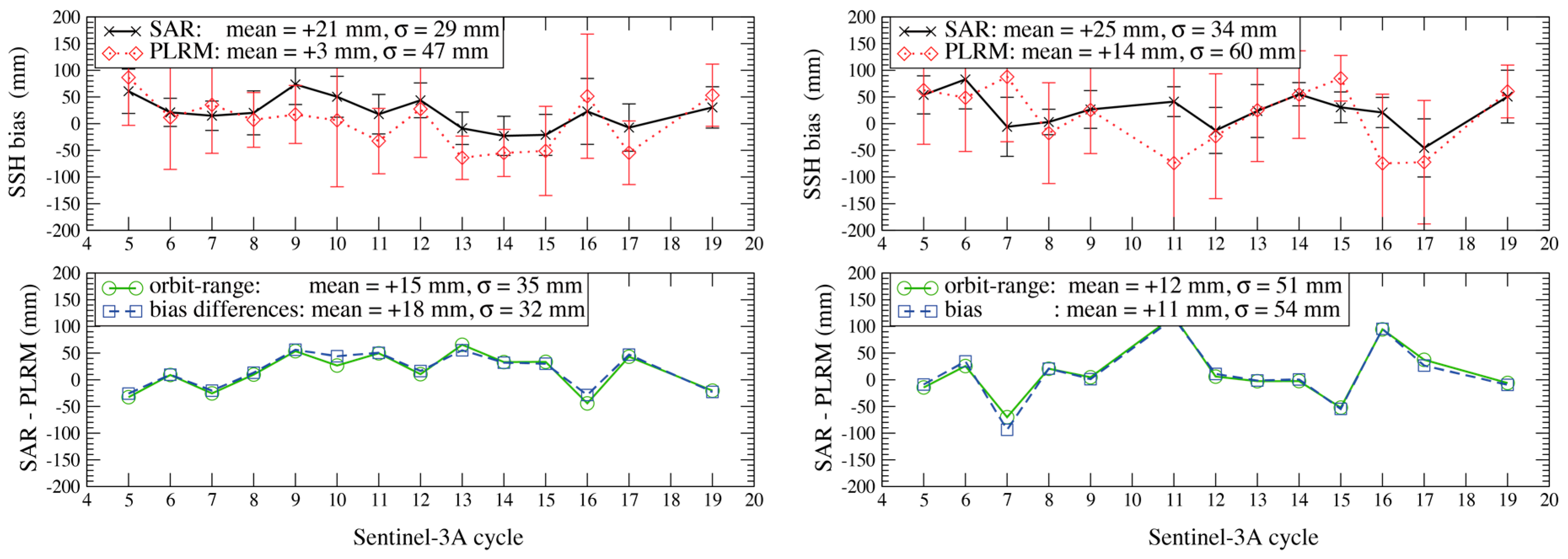
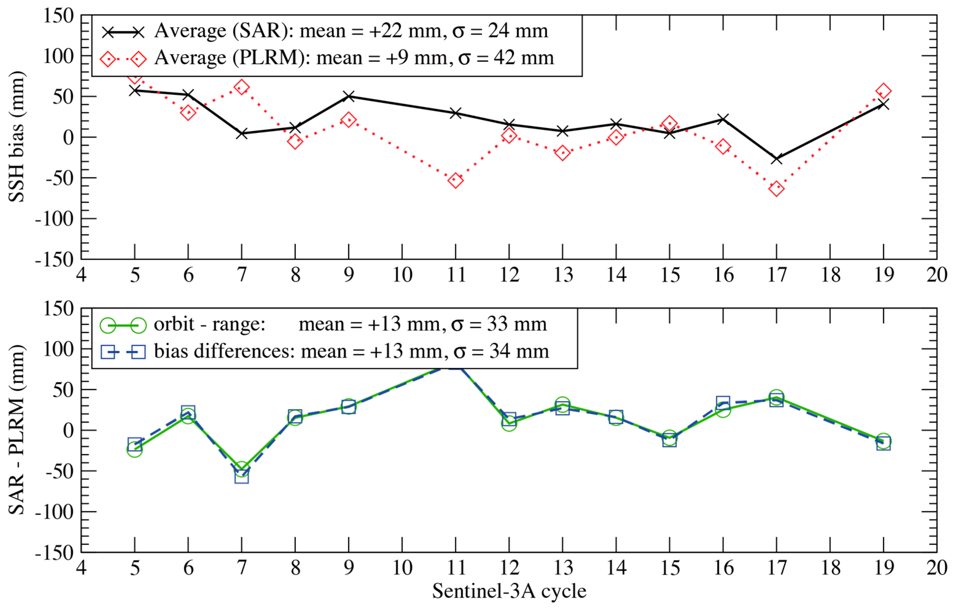
3.2. Sentinel-3A SSH Calibration and Corrections Validation
- -
- Sentinel-3A SAR: +22 ± 7 mm
- -
- Sentinel-3A PLRM: +9 ± 12 mm
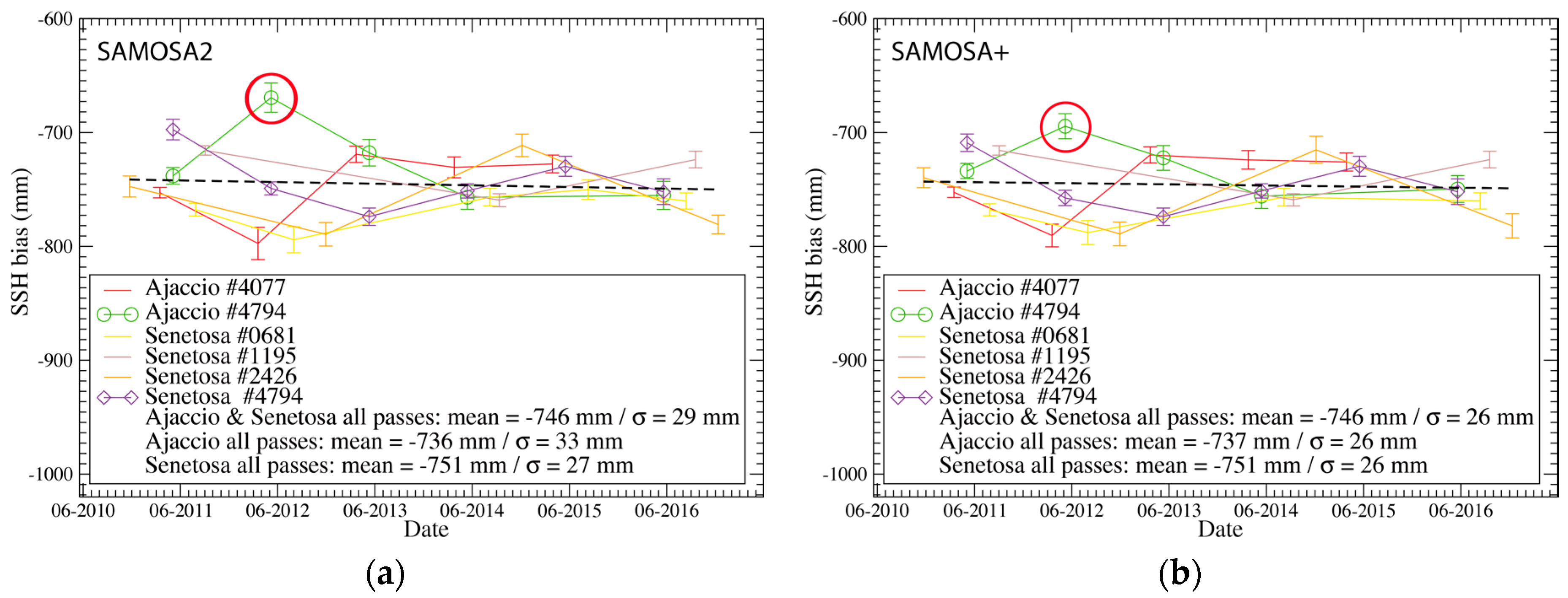
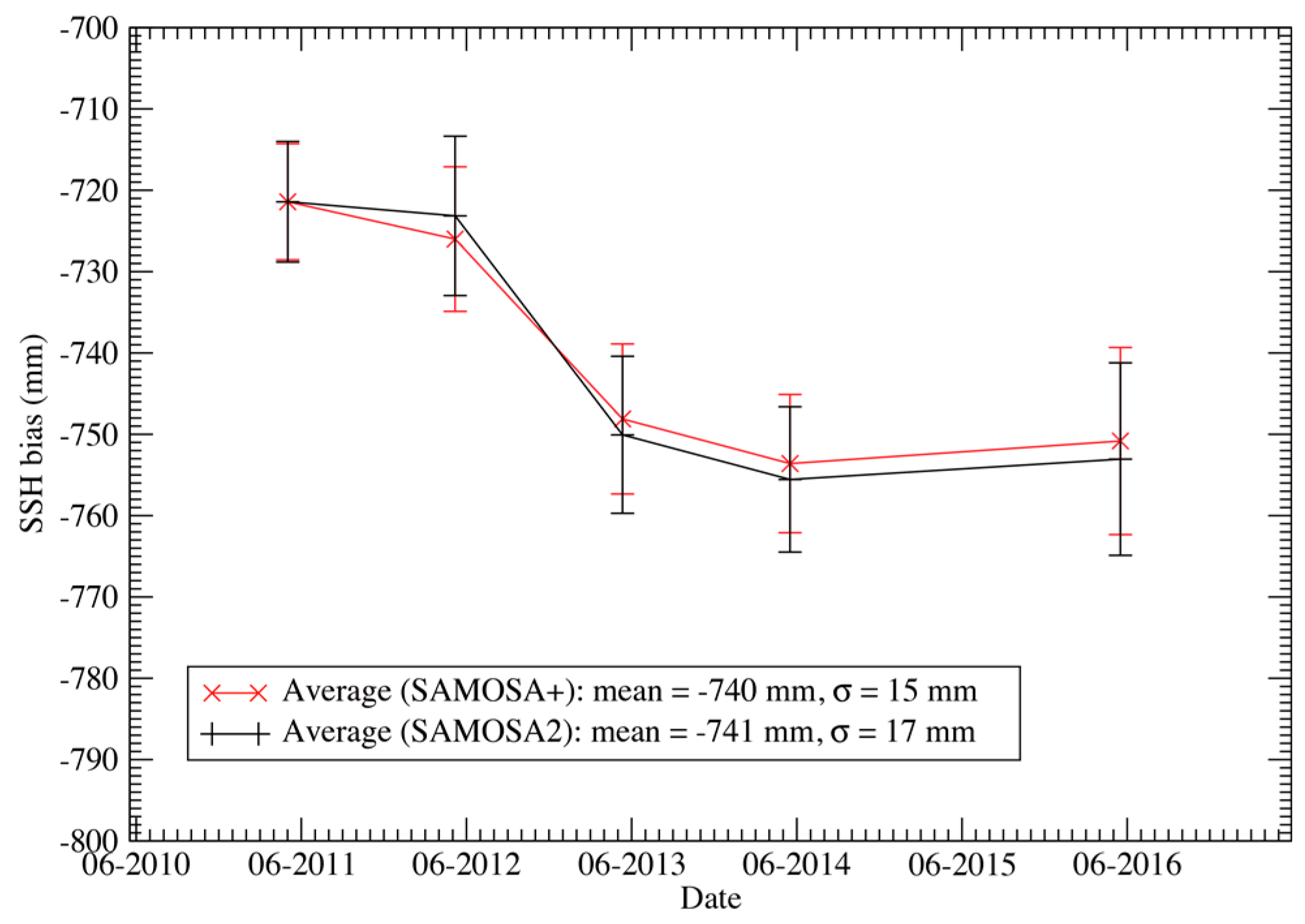
3.3. CryoSat-2 SSH Calibration
- -
- CryoSat-2 SAMOSA2: −746 ± 5.5 mm (−73 ± 5.5 mm for baseline C)
- -
- CryoSat-2 SAMOSA+: −746 ± 5.0 mm (−73 ± 5.0 mm for baseline C)
4. Discussion and Conclusions
Acknowledgments
Author Contributions
Conflicts of Interest
References
- Bonnefond, P.; Exertier, P.; Laurain, O.; Menard, Y.; Orsoni, A.; Jan, G.; Jeansou, E. Absolute Calibration of Jason-1 and TOPEX/Poseidon Altimeters in Corsica Special Issue on Jason-1 Calibration/Validation. Mar. Geod. 2003, 26, 261–284. [Google Scholar] [CrossRef]
- Bonnefond, P.; Exertier, P.; Laurain, O.; Jan, G. Absolute Calibration of Jason-1 and Jason-2 Altimeters in Corsica during the Formation Flight Phase. Mar. Geodesy 2010, 33, 80–90. [Google Scholar] [CrossRef]
- Bonnefond, P.; Laurain, O.; Exertier, P.; Guillot, A.; Picot, N.; Cancet, M.; Lyard, F. SARAL/AltiKa absolute calibration from the multi-mission Corsica facilities. Mar. Geodesy 2015, 38, 171–192. [Google Scholar] [CrossRef]
- Bonnefond, P.; Haines, B.; Watson, C. In Situ Calibration and Validation: A Link from Coastal to Open-ocean altimetry, chapter 11. In Coastal Altimetry; Vignudelli, S., Kostianoy, A., Cipollini, P., Benveniste, J., Eds.; Springer: Berlin/Heidelberg, Germany, 2011; pp. 259–296. ISBN 978-3-642-12795-3. [Google Scholar]
- Bonnefond, P.; Exertier, P.; Laurain, O.; Menard, Y.; Orsoni, A.; Jeansou, E.; Haines, B.; Kubitschek, D.; Born, G. Leveling Sea Surface using a GPS catamaran. Mar. Geodesy 2003, 26, 319–334. [Google Scholar] [CrossRef]
- Bonnefond, P.; Exertier, P.; Laurain, O.; Lyard, F.; Bijac, S.; Cancet, M.; Chimot, J.; Féménias, P. Corsica: An experiment for long-term Altimeter calibration and sea level monitoring. In Proceedings of the ESA Living Planet Symposium, Bergen, Norway, 28 June–2 July 2010. [Google Scholar]
- Bonnefond, P.; Verron, J.; Babu, K.N.; Bergé-Nguyen, M.; Cancet, M.; Chaudhary, A.; Crétaux, J.F.; Frappart, F.; Haines, B.J.; Laurain, O.; et al. The Benefits of the Ka-Band as Evidenced from the SARAL/AltiKa Altimetric Mission: Quality Assessment and Unique Characteristics of AltiKa Data. Remote Sens. 2017, 10, 83. [Google Scholar] [CrossRef]
- Donlon, C.; Berruti, B.; Buongiorno, A.; Ferreira, M.-H.; Féménias, P.; Frericka, J.; Goryl, P.; Kleina, U.; Laur, H.; Mavrocordatos, C.; et al. The Global Monitoring for Environment and Security (GMES) Sentinel-3 mission. Remote Sens. Environ. 2012, 120, 37–57. [Google Scholar] [CrossRef]
- Bouffard, J.; Webb, E.; Scagliola, M.; Garcia-Mondéjar, A.; Baker, S.; Brockley, D.; Gaudelli, J.; Muir, A.; Hall, A.; Mannan, R.; et al. CryoSat Instrument Performance and Ice Product Quality Status. Adv. Space Res. 2017. [Google Scholar] [CrossRef]
- Sentinel-3A SRAL Reprocessed Dataset Available on CODA from 16 October. Available online: https://www.eumetsat.int/website/home/News/DAT_3648215.html (accessed on 6 November 2017).
- Ray, C.; Martin-Puig, C.; Clarizia, M.P.; Ruffini, G.; Dinardo, S.; Gommenginger, C.; Benveniste, J. SAR altimeter backscattered waveform model. IEEE Trans. Geosci. Remote Sens. 2015, 53, 911–919. [Google Scholar] [CrossRef]
- Dinardo, S.; Fenoglio-Marc, L.; Buchhaupt, C.; Becker, M.; Scharroo, R.; Fernandez, J.M.; Benveniste, J. Coastal SAR and PLRM Altimetry in German Bight and West Baltic Sea. Adv. Space Res. 2017, in press. [Google Scholar] [CrossRef]
- Fenoglio-Marc, L.; Dinardo, S.; Scharroo, R.; Roland, A.; Dutour Sikiric, M.; Lucas, B.; Becker, M.; Benveniste, J.; Weiss, R. The German Bight: A validation of CryoSat-2 altimeter data in SAR mode. Adv. Space Res. 2015, 55, 2641–2656. [Google Scholar] [CrossRef]
- Chelton, D.B.; Walsh, E.J.; MacArthur, J.L. Pulse compression and sea level tracking in satellite altimetry. J. Atmos. Ocean. Technol. 1989, 6, 407–428. [Google Scholar] [CrossRef]
- King, R.; Bock, Y. Documentation for the GAMIT GPS Analysis Software. Release 10, Massachusetts Institute of Technology, Cambridge. 2000. Available online: http://www-gpsg.mit.edu/~simon/gtgk/GAMIT.pdf (accessed on 5 October 2017).
- Picard, B.; Fréry, M.; Pardé, M.; Bonnefond, P.; Laurain, O.; Crétaux, J.-F. A Wet Tropospheric Correction Dedicated to Hydrological and Coastal Applications. In Proceedings of the Ocean Surface Topography Science Team Meeting, Miami, FL, USA, 23–27 October 2017; Available online: https://meetings.aviso.altimetry.fr/fileadmin/user_upload/tx_ausyclsseminar/files/OSTST-2017_PICARD_NewCoastalNN_POSTER.pdf (accessed on 6 November 2017).
- Mertikas, S.; Donlon, C.; Mavrocordatos, C.; Féménias, P.; Galanakis, D.; Tziavos, I.; Boy, F.; Vergos, G.; Andersen, O.; Frantzis, X.; et al. Multi-mission calibrations results at the Permanent Facility for Altimetry Calibration in west Crete, Greece attaining Fiducial Reference Measurement Standards. In Proceedings of the Ocean Surface Topography Science Team Meeting, Miami, FL, USA, 23–27 October 2017; Available online: https://meetings.aviso.altimetry.fr/fileadmin/user_upload/tx_ausyclsseminar/files/OSTST_CalVal_20_Oct_2017_Mertikas_AAA.pdf (accessed on 6 November 2017).
- Garcia-Mondejar, A.; Mertikas, S.; Galanakis, D.; Labroue, S.; Bruniquel, J.; Quartly, G.; Féménias, P.; Mavrocordatos, C.; Wood, J.; Garcia, G.; et al. Sentinel-3 Transponder Calibration Results. In Proceedings of the Ocean Surface Topography Science Team Meeting, Miami, FL, USA, 23–27 October 2017; Available online: https://meetings.aviso.altimetry.fr/fileadmin/user_upload/tx_ausyclsseminar/files/S3_OSTST_Poster_20171012_V8.pdf (accessed on 6 November 2017).
- Dinardo, S. Guidelines for the SAR (Delay-Doppler) L1b Processing. 2013. Available online: http://wiki.services.eoportal.org/tiki-download_wiki_attachment.php?attId=2540 (accessed on 5 October 2017).
- Garcia-Mondejar, A.; Fornari, M.; Bouffard, J.; Féménias, P.; Roca, M. CryoSat-2: Range, Datation and Interferometer Calibration with Svalbard Transponder. Adv. Space Res. 2017. under review. [Google Scholar]


| Year | Reference Used | AJAC-G | Number of Days |
|---|---|---|---|
| 2005 | 50.0188 ± 0.0100 | ||
| 2013 | 50.0386 ± 0.0011 | 2 | |
| 2014 | 50.0360 ± 0.0010 | 3 | |
| 2015 | 50.0370 ± 0.0002 | 7 | |
| Average | 50.0371 ± 0.0004 |
| Radiometer-GPS | ||
|---|---|---|
| Mean | σ | |
| Senetosa | ||
| Standard product | −23 | 16 |
| CLS | −8 | 13 |
| Ajaccio | ||
| Standard product | −20 | 17 |
| CLS | −5 | 16 |
| Passes | SAMOSA2 | SAMOSA+ | Comment | ||||
|---|---|---|---|---|---|---|---|
| Mean (mm) | σ (mm) | Number of Cycles | Mean (mm) | σ (mm) | Number of Cycles | ||
| Ajaccio | |||||||
| 3563 | NA | NA | NA | NA | NA | NA | Coastal * |
| 4077 | −746 | 32 | 5 | −743 | 30 | 5 | Coastal * |
| 4794 | −727 | 36 | 5 | −731 | 24 | 5 | Coastal * |
| 5308 | NA | NA | NA | NA | NA | NA | Coastal * |
| Average | −736 | 33 | 10 | −737 | 26 | 10 | |
| Senetosa | |||||||
| 0681 | −766 | 17 | 5 | −768 | 14 | 4 | d > 3 km |
| 1195 | −733 | 23 | 3 | −733 | 23 | 3 | d > 8 km |
| 2426 | −757 | 36 | 4 | −756 | 35 | 4 | Coastal * |
| 4794 | −742 | 26 | 6 | −746 | 23 | 6 | d > 13 km |
| Average | −751 | 27 | 18 | −751 | 26 | 17 | |
| Total | −746 | 29 | 28 | −746 | 26 | 27 | |
© 2018 by the authors. Licensee MDPI, Basel, Switzerland. This article is an open access article distributed under the terms and conditions of the Creative Commons Attribution (CC BY) license (http://creativecommons.org/licenses/by/4.0/).
Share and Cite
Bonnefond, P.; Laurain, O.; Exertier, P.; Boy, F.; Guinle, T.; Picot, N.; Labroue, S.; Raynal, M.; Donlon, C.; Féménias, P.; et al. Calibrating the SAR SSH of Sentinel-3A and CryoSat-2 over the Corsica Facilities. Remote Sens. 2018, 10, 92. https://doi.org/10.3390/rs10010092
Bonnefond P, Laurain O, Exertier P, Boy F, Guinle T, Picot N, Labroue S, Raynal M, Donlon C, Féménias P, et al. Calibrating the SAR SSH of Sentinel-3A and CryoSat-2 over the Corsica Facilities. Remote Sensing. 2018; 10(1):92. https://doi.org/10.3390/rs10010092
Chicago/Turabian StyleBonnefond, Pascal, Olivier Laurain, Pierre Exertier, François Boy, Thierry Guinle, Nicolas Picot, Sylvie Labroue, Matthias Raynal, Craig Donlon, Pierre Féménias, and et al. 2018. "Calibrating the SAR SSH of Sentinel-3A and CryoSat-2 over the Corsica Facilities" Remote Sensing 10, no. 1: 92. https://doi.org/10.3390/rs10010092
APA StyleBonnefond, P., Laurain, O., Exertier, P., Boy, F., Guinle, T., Picot, N., Labroue, S., Raynal, M., Donlon, C., Féménias, P., Parrinello, T., & Dinardo, S. (2018). Calibrating the SAR SSH of Sentinel-3A and CryoSat-2 over the Corsica Facilities. Remote Sensing, 10(1), 92. https://doi.org/10.3390/rs10010092