Multi-Satellite Altimeter Validation along the French Atlantic Coast in the Southern Bay of Biscay from ERS-2 to SARAL


 , ,
, , 
Abstract
1. Introduction
2. Datasets and Study Area
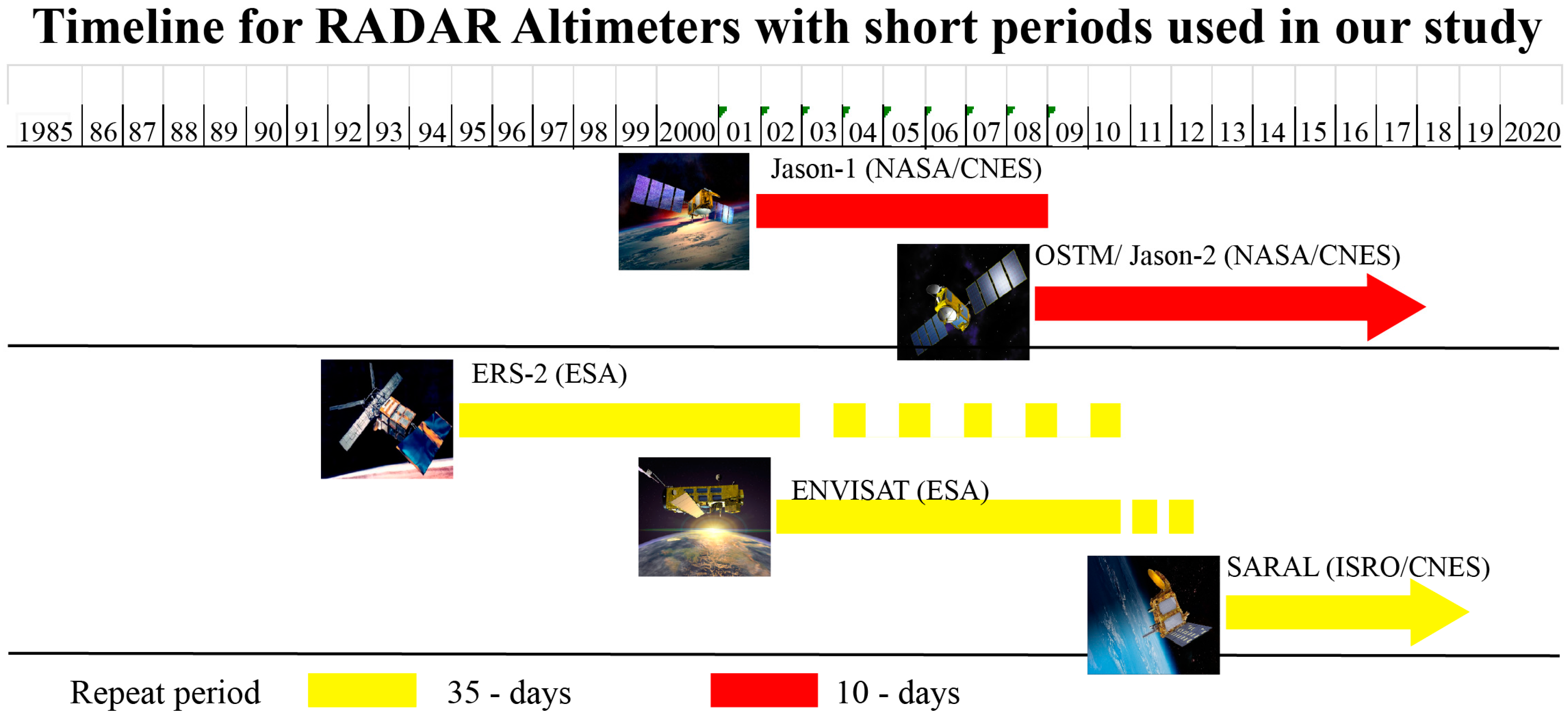
2.1. Radar Altimetry Data
2.1.1. Jason-1
2.1.2. Jason-2
2.1.3. ERS-2
2.1.4. Envisat
2.1.5. SARAL/AltiKa
2.2. Tide Gauge Records
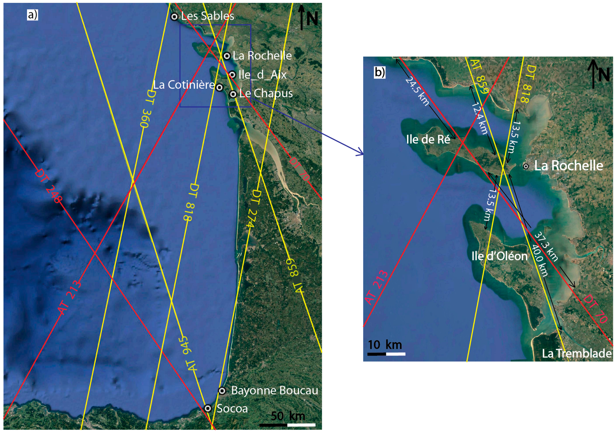
2.3. Study Area
3. Methods
3.1. SSH from Altimetry
3.2. SSH Processing and Editing
3.3. Comparisons between Altimetry-Based and In Situ-Based SSH
3.4. Comparisons of the Atmosphere Delays over the Open Ocean
4. Results
4.1. Multi-Missions Comparisons over the French Southern Part of the Bay of Biscay
4.2. Multi-Mission Comparisons at La Rochelle Tide Gauge
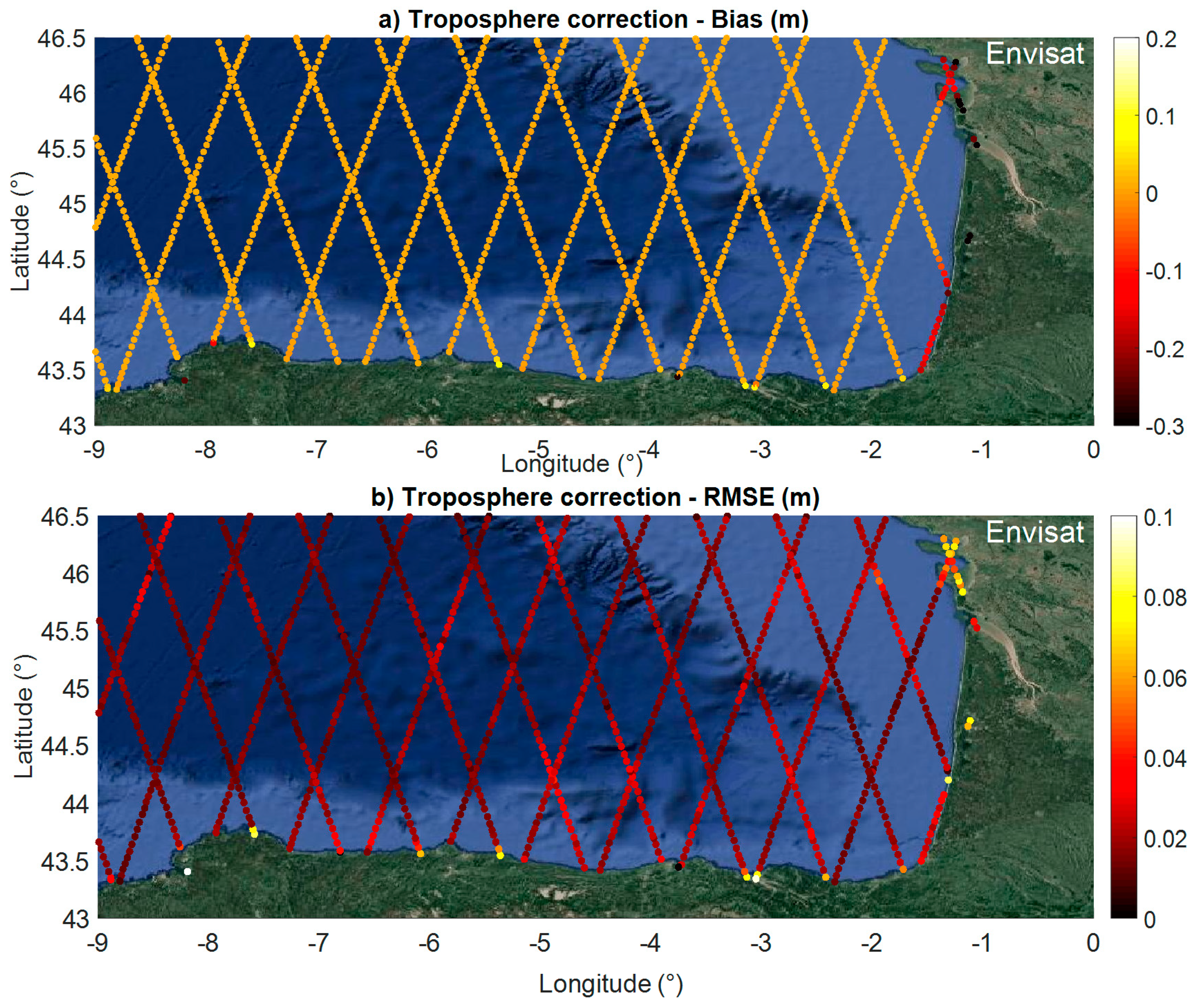
4.3. Comparisons of Atmosphere Corrections over the Open Ocean
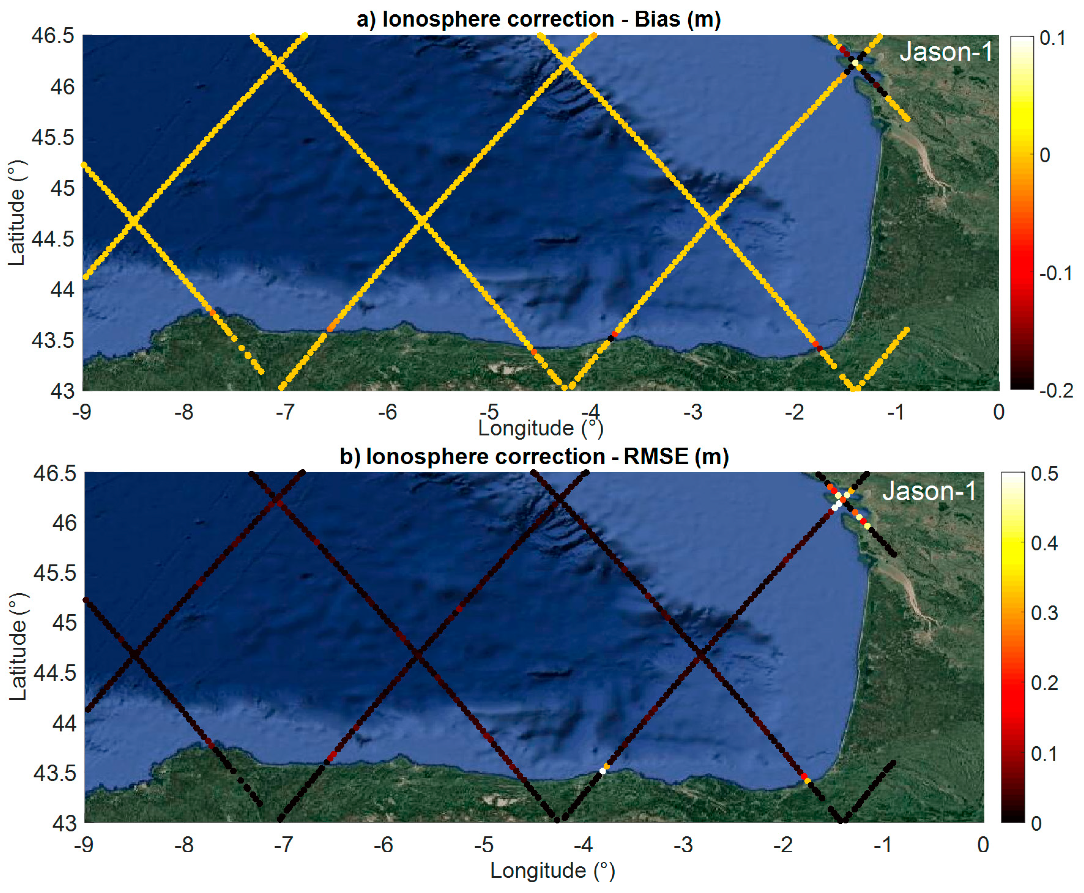
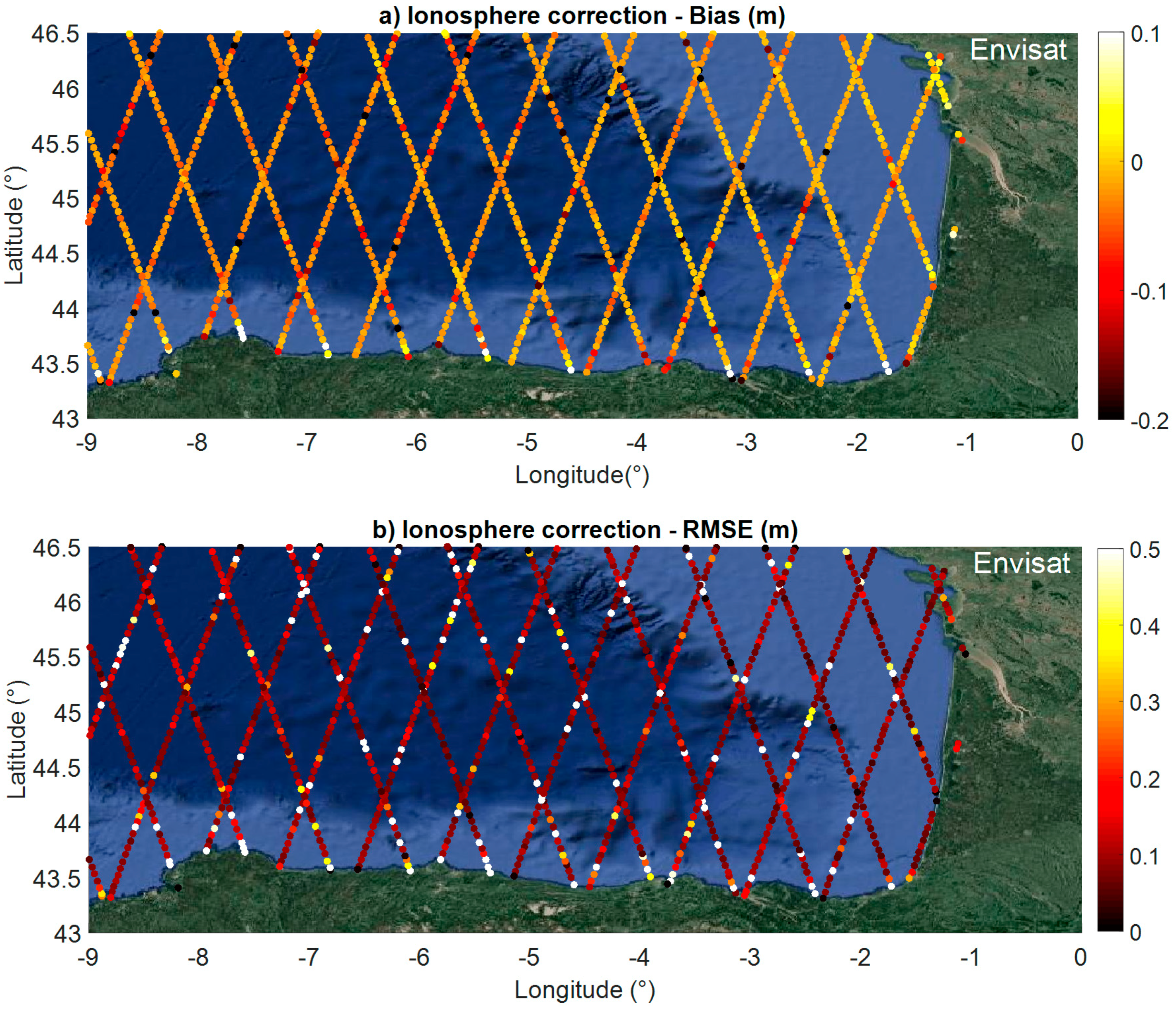
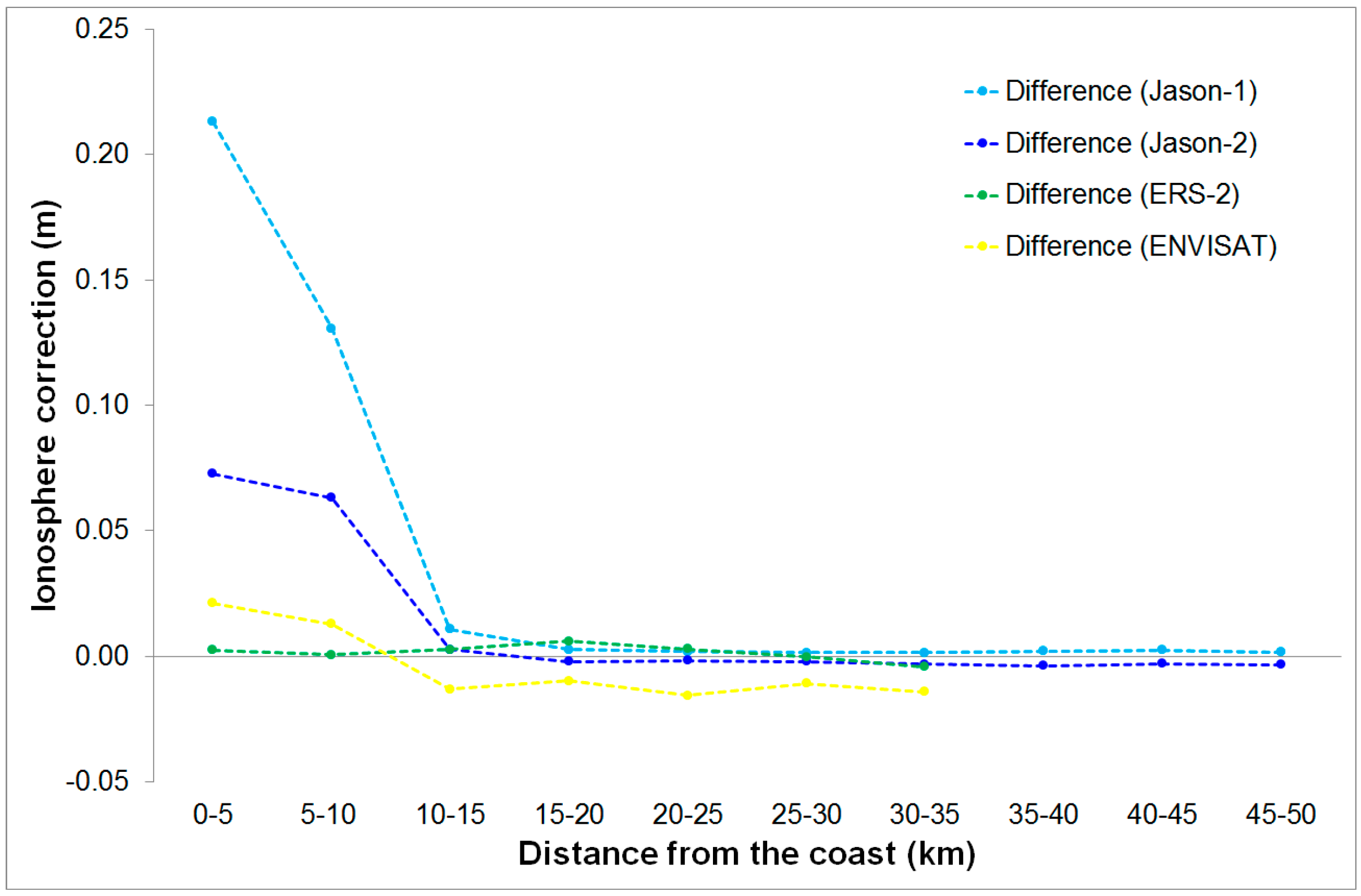
4.3.1. Comparisons of Bi-Frequency and Model-Based Ionospheric Corrections
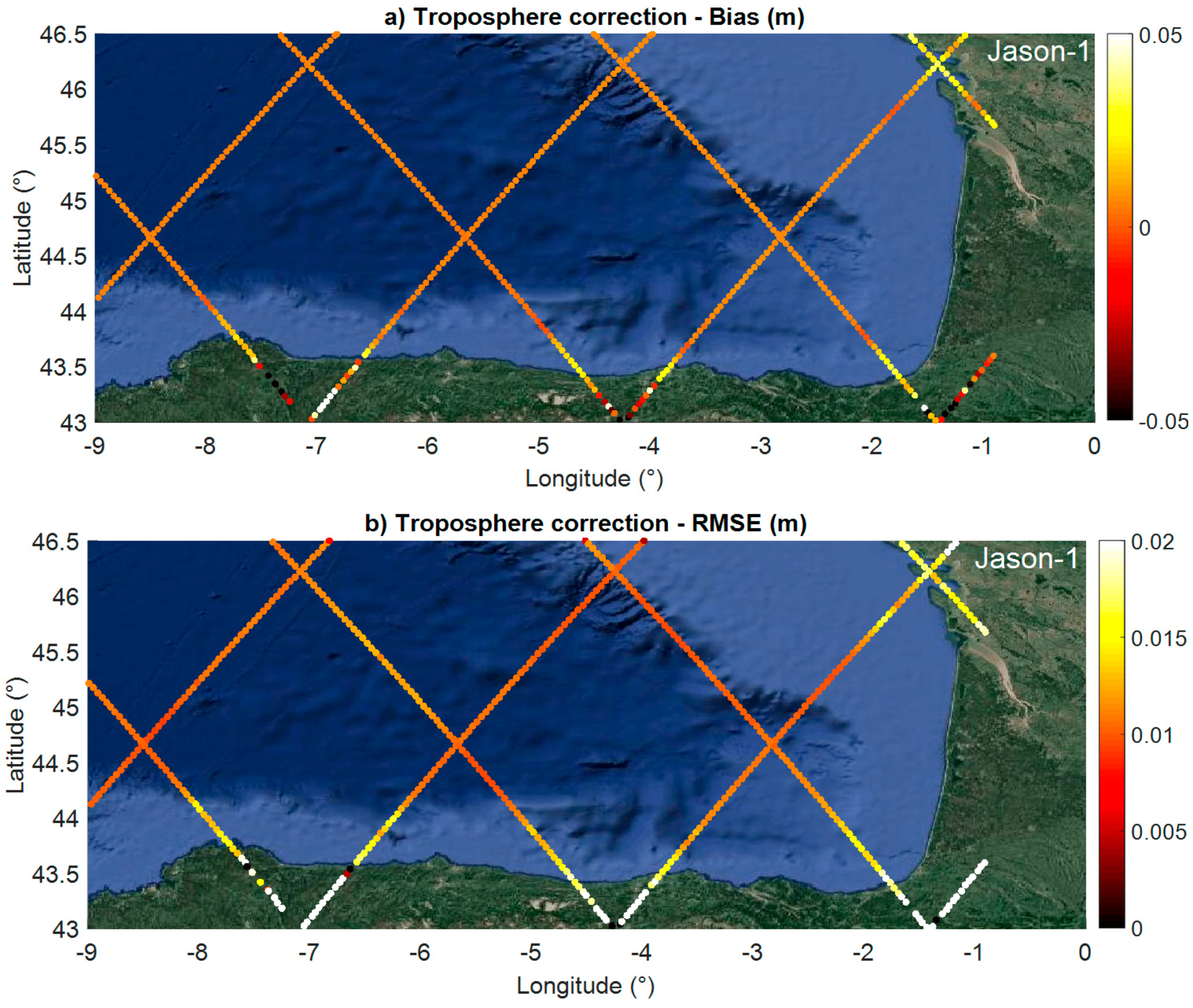
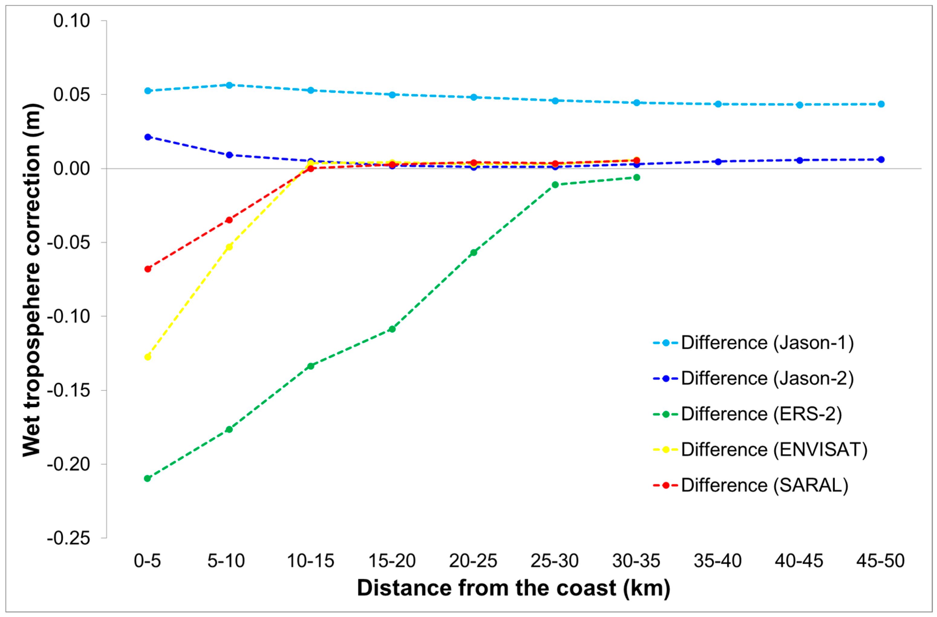
4.3.2. Wet Tropospheric Correction Comparison between Radiometers and ECMWF Model
5. Discussion
6. Conclusions
Supplementary Materials
Acknowledgments
Author Contributions
Conflicts of Interest
References
- Fu, L.L.; Cazenave, A. Satellite Altimetry and Earth Sciences: A Handbook of Techniques and Applications; International Geophysics Series; Academic Press: San Diego, CA, USA, 2001; Volume 69, 463p. [Google Scholar]
- Frappart, F.; Blumstein, D.; Cazenave, A.; Ramillien, G.; Birol, F.; Morrow, R.; Rémy, F. Satellite Altimetry: Principles and Applications in Earth Sciences. In Wiley Encyclopedia of Electrical and Electronics Engineering; Webster, J., Ed.; John Wiley & Sons: Hoboken, NJ, USA, 2017; pp. 1–25. [Google Scholar]
- Deng, X.; Featherstone, W.E.; Hwang, C.; Berry, P.A.M. Estimation of contamination of ERS-2 and POSEIDON satellite radar altimetry close to the coasts of Australia. Mar. Geodesy 2002, 25, 249–271. [Google Scholar] [CrossRef]
- Deng, X.; Featherstone, W.E. A coastal retracking system for satellite radar altimeter waveforms: Application to ERS-2 around Australia. J. Geophys. Res. 2006, 111. [Google Scholar] [CrossRef]
- Gommenginger, C.; Thibaut, P.; Fenoglio-Marc, L.; Qyartly, G.; Deng, X.; Gomez-Enri, J.; Challenor, P.; Gao, Y. Retracking altimeter waveforms near the coasts: A review of retracking methods and some applications to coastal waveforms. In Coastal Altimetry; Vignudelli, S., Kostianoy, A., Cipollini, P., Benveniste, J., Eds.; Springer: Berlin/Heidelberg, Germany, 2011; pp. 61–101. [Google Scholar]
- Bonnefond, P.; Exertier, P.; Laurain, O.; Thibaut, P.; Mercier, F. GPS-based sea level measurements to help the characterization of land contamination in coastal areas. Adv. Space Res. 2013, 51, 1383–1399. [Google Scholar] [CrossRef]
- Andersen, O.B.; Scharroo, R. Range and geophysical corrections in coastal regions: And implications for mean sea surface determination. In Coastal Altimetry; Vignudelli, S., Kostianoy, A., Cipollini, P., Benveniste, J., Eds.; Springer: Berlin/Heidelberg, Germany, 2011; pp. 103–146. [Google Scholar]
- Robinson, A.R.; Brink, K.H. The Global Coastal Ocean: Multiscale Interdisciplinary Processes. In The Sea; Harvard University Press: Cambrige, UK, 2005; Volume 13, p. 1062. [Google Scholar]
- Verron, J.; Sengenes, P.; Lambin, J.; Noubel, J.; Steunou, N.; Guillot, A.; Picot, N.; Coutin-Faye, S.; Gairola, R.; Raghava Murthy, D.V.A.; et al. The SARAL/AltiKa altimetry satellite mission. Mar. Geodesy 2015, 38, 2–21. [Google Scholar] [CrossRef]
- Wingham, D.J.; Francis, C.R.; Baker, S.; Bouzinac, C.; Brockley, D.; Cullen, R.; de Chateau-Thierry, P.; Laxon, S.W.; Mallow, U.; Mavrocordatos, C.; et al. CryoSat: A mission to determine the fluctuations in Earth’s land and marine ice fields. Adv. Space Res. 2006, 37, 841–871. [Google Scholar] [CrossRef]
- Obligis, E.; Desportes, C.; Eymard, L.; Fernandes, M.J.; Lázaro, C.; Nunes, A. Tropospheric Corrections for Coastal Altimetry. In Coastal Altimetry; Vignudelli, S., Kostianoy, A., Cipollini, P., Benveniste, J., Eds.; Springer: Berlin/Heidelberg, Germany, 2011; pp. 147–176. [Google Scholar]
- Passaro, M.; Cipollini, P.; Vignudelli, S.; Quartly, G.D.; Snaith, H.M. ALES: A multi-mission subwaveform retracker for coastal and open ocean altimetry. Remote Sens. Environ. 2014, 145, 173–189. [Google Scholar] [CrossRef]
- Fernandes, M.J.; Lázaro, C.; Nunes, A.L.; Scharroo, R. Atmospheric Corrections for Altimetry Studies over Inland Water. Remote Sens. 2014, 6, 4952–4997. [Google Scholar] [CrossRef]
- Birol, F.; Fuller, N.; Lyard, F.; Cancet, M.; Niño, F.; Delebecque, C.; Fleury, S.; Toublanc, F.; Melet, A.; Saraceno, M. Coastal applications from nadir altimetry: Example of the X-TRACK regional products. Adv. Space Res. 2017, 59, 936–953. [Google Scholar] [CrossRef]
- Bonnefond, P.; Exertier, P.; Laurain, O.; Ménard, Y.; Orsoni, A.; Jan, G.; Jeansou, E. Absolute Calibration of Jason-1 and TOPEX/Poseidon Altimeters in Corsica. Mar. Geodesy 2003, 26, 261–284. [Google Scholar] [CrossRef]
- Haines, B.J.; Desai, S.D.; Born, G.H. The Harvest experiment of the climate data record from TOPEX/Poseidon, Jason-1 and the ocean surface topography mission. Mar. Geodesy 2010, 33, 91–113. [Google Scholar] [CrossRef]
- Mertikas, S.P.; Ioannides, R.T.; Tziavos, I.N.; Vergos, G.S.; Hausleitner, W.; Frantzis, X.; Tripolitsiotis, A.; Partsinevelos, P.; Andrikopoulos, D. Statistical models and latest results in the determination of the absolute bias for the radar altimeters of Jason satellites using the Gavdos facility. Mar. Geodesy 2010, 33, 114–149. [Google Scholar] [CrossRef]
- Watson, C.S.; White, N.C.; Church, J.A.; Burgette, R.J.; Tregoning, P.; Coleman, R. Absolute calibration in Bass Strait, Australia: TOPEX, Jason-1 and OSTM/Jason-2. Mar. Geodesy 2011, 34, 242–260. [Google Scholar] [CrossRef]
- Pingree, R.D.; Mardell, G.T.; New, A.L. Propagation of internal tides from the upper slopes of the Bay of Biscay. Nature 1986, 321, 154–158. [Google Scholar] [CrossRef]
- New, A.L. Internal tidal mixing in the Bay of Biscay. Deep Sea Res. Part A Oceanogr. Res. Pap. 1988, 35, 691–709. [Google Scholar] [CrossRef]
- Pairaud, I.L.; Lyard, F.; Auclair, F.; Letellier, T.; Marsaleix, P. Dynamics of the semi-diurnal and quarter-diurnal internal tides in the Bay of Biscay. Part 1: Barotropic tides. Cont. Shelf Res. 2008, 28, 1294–1315. [Google Scholar] [CrossRef]
- Iijima, B.A.; Harris, I.L.; Ho, C.M.; Lindqwister, U.J.; Mannucci, A.J.; Pi, X.; Reyes, M.J.; Sparks, L.C.; Wilson, B.D. Automated daily process for global ionospheric total electron content maps and satellite ocean altimeter ionospheric calibration based on Global Positioning System data. J. Atmos. Sol.-Terr. Phys. 1999, 61, 1205–1218. [Google Scholar] [CrossRef]
- Scharroo, R.; Smith, W.H.F. Global positioning system-based climatology for the total electron content in the ionosphere. J. Geophys. Res. 2010, 115. [Google Scholar] [CrossRef]
- CTOH: Centre for Topographic Studies of the Oceans and Hydrosphere. Available online: http://ctoh.legos.obs-mip.fr (accessed on 4 December 2017).
- United States Department of Agriculture. Available online: https://ipad.fas.usda.gov/cropexplorer/global_reservoir (accessed on 4 December 2017).
- Carayon, G.; Steunou, N.; Courrière, J.; Thibaut, P. Poseidon-2 radar altimeter design and results of in-flight performances. Mar. Geodesy 2003, 26, 159–165. [Google Scholar] [CrossRef]
- Desjonquères, J.-D.; Carayon, G.; Steunou, N.; Lambin, J. Poseidon-3 Radar Altimeter: New Modes and In-Flight Performances. Mar. Geodesy 2010, 33, 53–79. [Google Scholar] [CrossRef]
- Zelli, C. ENVISAT RA-2 advanced radar altimeter: Instrument design and prelaunch performance assessment review. Acta Astronaut. 1999, 44, 323–333. [Google Scholar] [CrossRef]
- Service Hydrographique et Océanographique de la Marine. Available online: http://data.shom.fr/donnes/refmar (accessed on 4 December 2017).
- Besser, G. Marées; Service Hydrographique et Océanographique de la Marine: Paris, France, 1985. [Google Scholar]
- Charria, G.; Lazure, P.; le Cann, B.; Serpette, A.; Reverdin, G.; Louazel, S.; Batifoulier, F.; Dumas, F.; Pichon, A.; Morele, Y. Surface layer circulation derived from Lagrangian drifters in the Bay of Biscay. J. Mar. Syst. 2013, 109, 60–76. [Google Scholar] [CrossRef]
- Frouin, R.; Fiúza, A.F.G.; Ambar, I.; Boyd, T.J. Observations of a Poleward Surface Current off the Coasts of Portugal and Spain During Winter. J. Geophys. Res. 1990, 95, 679–691. [Google Scholar] [CrossRef]
- Le Cann, B.; Pingree, R.D. Structure, strength, and seasonality of the slope current in the Bay of Biscay region. J. Mar. Biol. Assoc. 1990, 70, 857–885. [Google Scholar]
- Lazune, P.; Jegou, A.-M.; Kerdreux, M. Analysis of salinity measurements near islands on the French continental shelf of the Bay of Biscay. Sci. Mar. 2006, 70, 7–14. [Google Scholar]
- Pichon, A.; Correard, S. Internal tides modelling in the Bay of Biscay. Comparisons with observations. Sci. Mar. 2006, 70, 65–88. [Google Scholar] [CrossRef]
- Ménard, Y.; Jeansou, E.; Vincent, P. Calibration of the TOPEX/POSEIDON Altimeters Additional Results at Harvest. J. Geophys. Res. 1994, 99, 24487–24504. [Google Scholar] [CrossRef]
- Chelton, D.B.; Ries, J.C.; Haines, B.J.; Fu, L.-L.; Callahan, P.S. Satellite Altimetry. In Satellite Altimetry and Earth Sciences; Fu, L.-L., Cazenave, A., Eds.; Academic Press: San Diego, CA, USA, 2001; pp. 1–131. [Google Scholar]
- Frappart, F.; Papa, F.; Marieu, V.; Malbéteau, Y.; Jordy, F.; Calmant, S.; Durand, F.; Bala, S. Preliminary assessment of SARAL/AltiKa observations over the Ganges-Brahmaputra and Irrawaddy Rivers. Mar. Geodesy 2015, 38, 568–580. [Google Scholar] [CrossRef]
- Frappart, F.; Roussel, N.; Biancale, R.; Martinez Benjamin, J.J.; Mercier, F.; Pérosanz, F.; Garate Pasquin, J.; Martin Davila, J.; Perez Gomez, B.; Gracia Gomez, C.; et al. The 2013 Ibiza calibration campaign of Jason-2 and SARAL altimeters. Mar. Geodesy 2015, 38, 219–232. [Google Scholar] [CrossRef]
- Frappart, F.; Legrésy, B.; Niño, F.; Blarel, F.; Fuller, N.; Fleury, S.; Birol, F.; Calmant, S. An ERS-2 altimetry reprocessing compatible with ENVISAT for long-term land and ice sheets studies. Remote Sens. Environ. 2016, 184, 558–581. [Google Scholar] [CrossRef]
- Biancamaria, S.; Frappart, F.; Leleu, A.S.; Marieu, V.; Blumstein, D.; Boy, F.; Sottolichio, A.; Valle-Levinson, A. Satellite radar altimetry water elevations performance over a hundred meter wide river: Evaluation over the Garonne River. Adv. Space Res. 2017, 59, 128–146. [Google Scholar] [CrossRef]
- Amarouche, L.; Thibaut, P.; Zanife, O.Z.; Dumont, J.-P.; Vincent, P.; Steunou, N. Improving the Jason-1 ground retracking to better account for attitude effects. Mar. Geodesy 2004, 27, 171–197. [Google Scholar] [CrossRef]
- Rodríguez, E. Altimetry for non-Gaussian oceans: Height biases and estimation of parameters. J. Geophys. Res. 1988, 93, 14107–14120. [Google Scholar] [CrossRef]
- Brown, G. The average impulse response of a rough surface and its applications. IEEE Trans. Antennas Propag. 1977, 25, 67–74. [Google Scholar] [CrossRef]
- Astudillo, O.; Dewitte, B.; Mallet, M.; Frappart, F.; Rutllant, J.; Ramos, M.; Bravo, L.; Goubanova, K.; Illig, S. Surface winds off Peru-Chile: Observing closer to the coast from radar altimetry. Remote Sens. Environ. 2017, 191, 179–196. [Google Scholar] [CrossRef]
- Blarel, F.; Frappart, F.; Legrésy, B.; Blumstein, D.; Rémy, F.; Fatras, C.; Mougin, E.; Papa, F.; Prigent, C.; Niño, F.; et al. Altimetry backscattering signatures at Ku and S bands over land and ice sheets. In Remote Sensing for Agriculture, Ecosystems, and Hydrology XVII; Neale, C.M.U., Maltese, A., Eds.; Society of Photo-Optical Instrumentation Engineers (SPIE): Bellingham, WA, USA, 2015. [Google Scholar]
- Martin-Puig, C.; Leuliette, E.; Lillibridge, J.; Roca, M. Evaluating the Performance of Jason-2 Open-Loop and Closed-Loop Tracker Modes. Am. Meteorol. Soc. 2016. [Google Scholar] [CrossRef]
- Vignudelli, S.; Kostianoy, A.G.; Cipollini, P.; Benveniste, J. Coastal Altimetry; Springer-Verlag: Berlin/Heidelberg, Germany, 2011; p. 578. [Google Scholar]
- Brown, S. A Novel Near-Land Radiometer Wet Path-Delay Retrieval Algorithm: Application to the Jason-2/OSTM Advanced Microwave Radiometer. Geosci. Remote Sens. 2010, 48, 1986–1992. [Google Scholar] [CrossRef]
- Bonnefond, P.; Verron, J.; Aublanc, J.; Babu, K.N.; Bergé-Nguyen, M.; Cancet, M.; Chaudhary, A.; Crétaux, J.-F.; Frappart, F.; Haines, B.J.; et al. The Benefits of the Ka-Band as Evidenced from the SARAL/AltiKa Altimetric Mission: Quality Assessment and Unique Characteristics of AltiKa Data. Remote Sens. 2018, 10, 83. [Google Scholar] [CrossRef]
- Liu, Y.; Kerkering, H.; Weisberg, R.H. Coastal Ocean Observing Systems; Elsevier: Amsterdam, The Netherlands, 2015; p. 461. ISBN 978-0-12-802022-7. [Google Scholar]


| Tide Gauge Station | Longitude (°) | Latitude (°) | Validation Period | ZH/GRS80 (m) | Jason-1 and 2 | ERS-2, Envisat, SARAL | ||
|---|---|---|---|---|---|---|---|---|
| Track | Distance (km) | Track | Distance (km) | |||||
| Bayonne Boucau | 43.5273 | −1.5148 | 1999–2015 | 46.41 | 248 | 24.3 | 274, 945 | 3.0, 18.6 |
| Bourceranc le Chapus | 45.8534 | −1.1778 | 2012–2013 | 43.49 | 70 | 7.0 | 818, 859 | 17.8, <1 |
| Ile d’Aix | 46.0074 | −1.1743 | 2011–2015 | 43.49 | 70, 213 | 2.88, 29.0 | 818, 859 | 13.7, 4.7 |
| La Rochelle la Pallice | 46.1585 | −1.2206 | 1996–2015 | 43.46 | 70, 213 | 8.8, 16.8 | 818, 859 | 5.8, 5.4 |
| Les Sables d’Olonne | 46.4974 | −1.7935 | 1995–2015 | 44.54 | 70 | 7.0 | 360 | 6.6 |
| La Cotinière | 45.9136 | −1.3278 | 2006–2015 | 43.45 | 213 | 24.8 | 818 | 4.7 |
| Saint Jean de Luz Socoa | 43.3952 | −1.6816 | 2002–2015 | 46.64 | 248 | 5.4 | 274, 945 | 6.2, 2.1 |
| Altimetry Mission | Period | Format | Ocean Retracking Algorithm | Corrections to the Range | |||
|---|---|---|---|---|---|---|---|
| Ionosphere | Dry Troposphere | Wet Troposphere | Sea State Bias | ||||
| ERS-2 | Cycle 1 (May 1995) to cycle 085 (July 2003) | REAPER GDR | MLE-3 | NIC 09 GIM | ECMWF | Radiometer ECMWF | Empirical |
| Jason-1 | Cycle 001 (January 2002) to cycle 259 (January 2009) | GDR E | MLE-3 | Bi-frequency (C-Ku) GIM model | ECMWF model derived | Jason-1 radiometer (JMR) and ECMWF model | Empirical model derived |
| Envisat | Cycle 006 (May 2002) to cycle 094 (October 2010) | GDR C v2.1 | MLE-3 | Bi-frequency (C-Ku) GIM model | ECMWF model derived | Microwave Radiometer (MWR) and ECMWF model | Empirical model derived |
| Jason-2 | Cycle 001 (July 2008) to cycle 250 (April 2015) | GDR D | MLE-4 MLE-3 | Bi-frequency (C-Ku) and GIM model | ECMWF atmospheric pressures | Jason-2 radiometer (AMR) and ECMWF model | Empirical model derived from Jason-2 data |
| SARAL | Cycle 001 (March 2013) to cycle 028 (November 2015) | GDR T | MLE-4 | GIM- derived | ECMWF model derived | Radiometer and ECMWF model | Empirical model derived |
| Altimeter | Station | Altimetry Track | Distance Alt/Gauge (km) | N | Bias (m) | RMSE (m) | SD (m) | R |
|---|---|---|---|---|---|---|---|---|
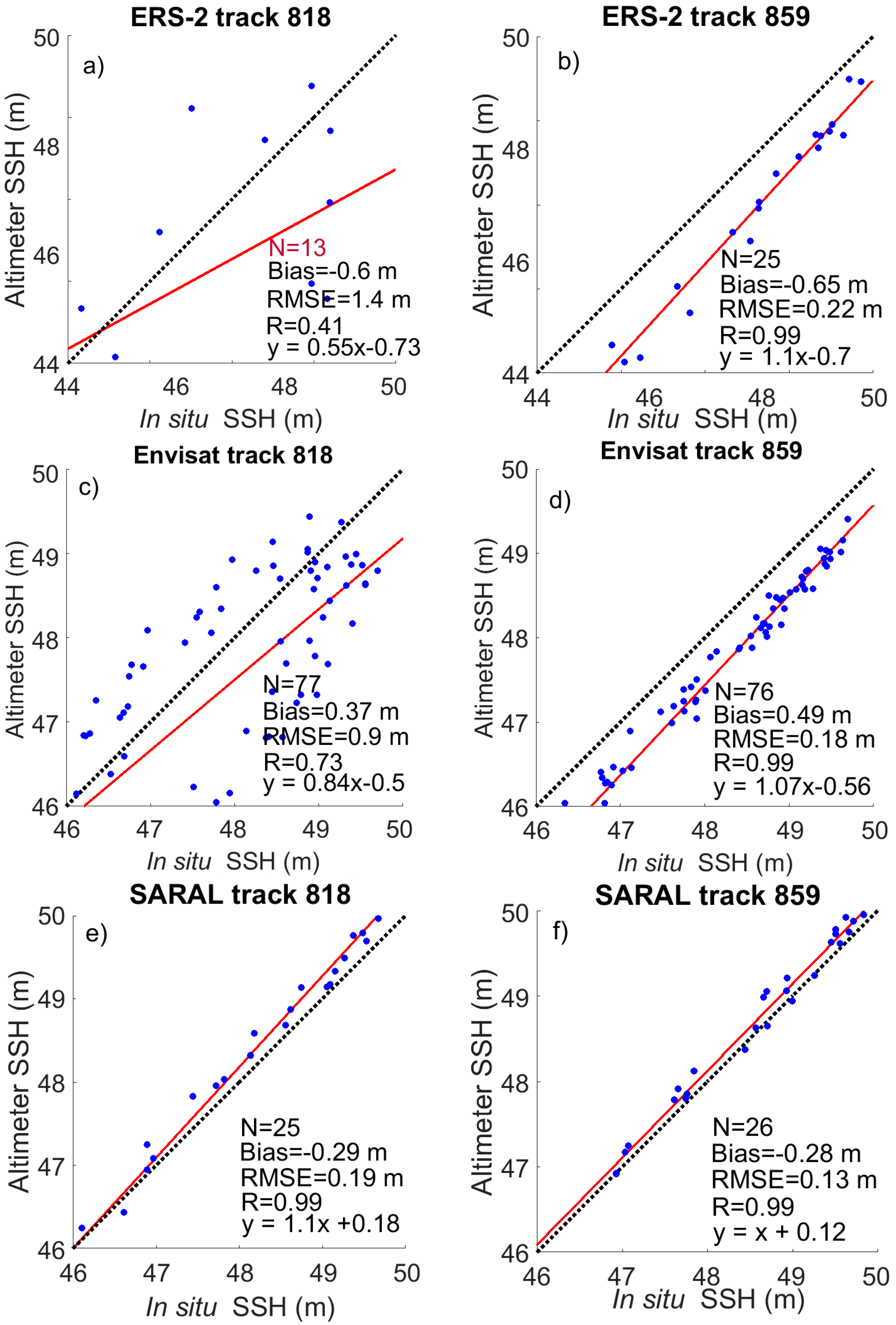
| La Rochelle | 818 | 5.8 | 13 | −0.6 | 1.4 | 1.05 | 0.41 | |
| ERS-2 | La Rochelle | 859 | 5.4 | 25 | −0.65 | 0.22 | 1.45 | 0.99 |
| Bayonne Boucau | 274 | 3.0 | 21 | −1.00 | 0.89 | 1.05 | 0.51 | |
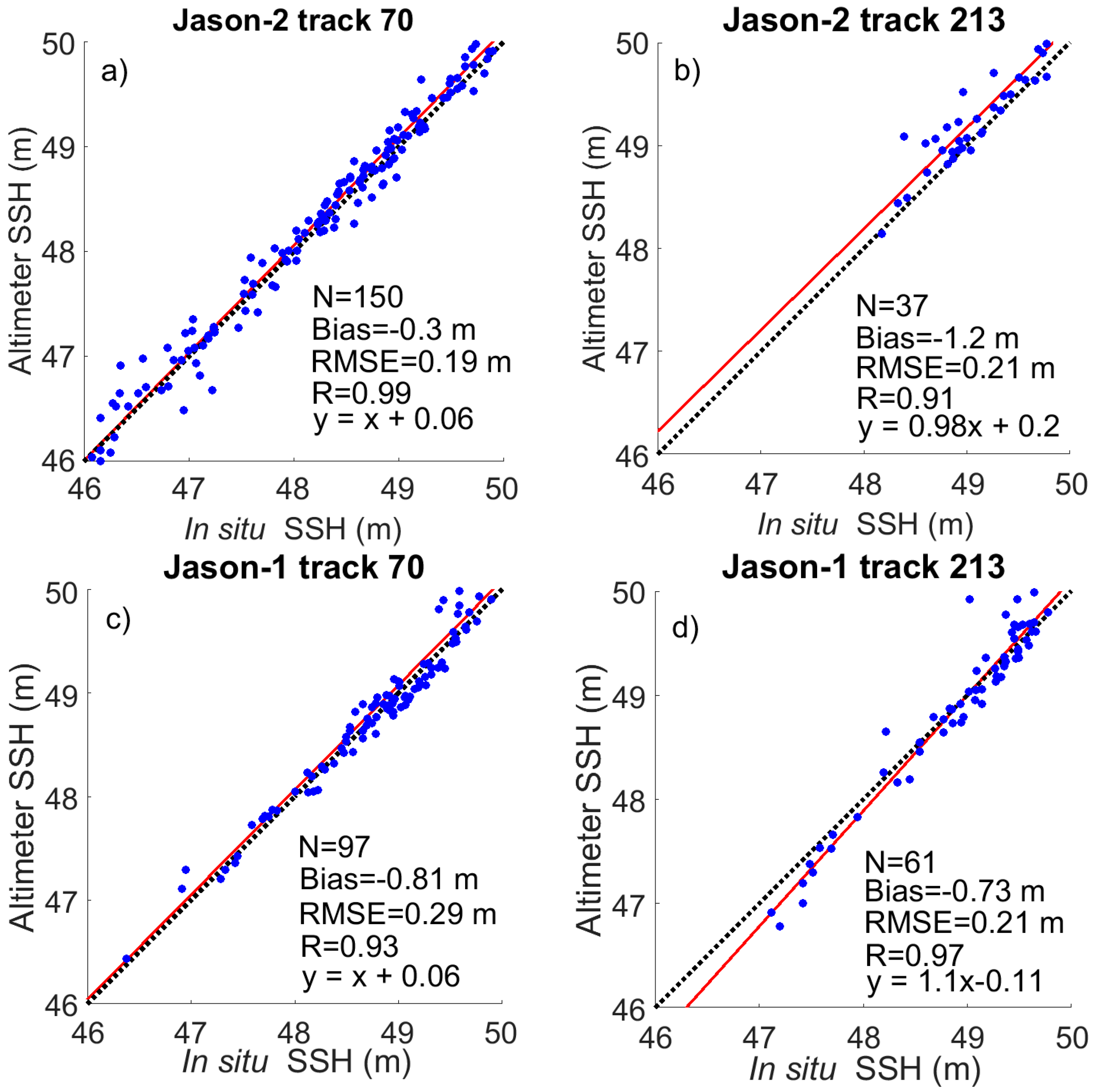
| La Rochelle | 70 | 8.8 | 97 | −0.81 | 0.29 | 0.98 | 0.93 | |
| Jason-1 | La Rochelle | 213 | 16.8 | 61 | −0.73 | 0.21 | 0.71 | 0.97 |
| Bayonne Boucau | 248 | 24.3 | 25 | −0.94 | 0.15 | 1.00 | 0.99 | |
| Saint Jean de Luz Socoa | 248 | 5.4 | 35 | −0.77 | 0.10 | 1.00 | 0.996 | |
| La Rochelle | 818 | 5.8 | 77 | 0.37 | 0.90 | 1.00 | 0.73 | |
| La Rochelle | 859 | 5.4 | 76 | 0.49 | 0.18 | 1.15 | 0.99 | |
| Envisat | Bayonne Boucau | 274 | 3.0 | 42 | −0.07 | 0.77 | 0.99 | 0.67 |
| Saint Jean de Luz Socoa | 274 | 6.2 | 51 | −0.17 | 0.63 | 0.99 | 0.8 | |
| Les Sables d’Olonne | 360 | 6.6 | 38 | 0.25 | 0.84 | 0.97 | 0.7 | |
| La Rochelle | 70 | 8.8 | 150 | −0.30 | 0.19 | 0.99 | 0.99 | |
| La Rochelle | 213 | 16.8 | 37 | −1.20 | 0.21 | 1.27 | 0.91 | |
| Bayonne Boucau | 248 | 24.3 | 118 | −0.65 | 0.34 | 1.03 | 0.93 | |
| Jason-2 | Saint Jean de Luz Socoa | 248 | 5.4 | 84 | −0.78 | 0.33 | 1.03 | 0.92 |
| Les Sables d’Olonne | 70 | 7.0 | 111 | −0.67 | 0.17 | 0.99 | 0.98 | |
| Ile d’Aix | 213 | 29.0 | 14 | −1.1 | 0.27 | 1.27 | 0.83 | |
| Ile d’Aix | 70 | 2.88 | 58 | −0.37 | 0.21 | 1.44 | 0.98 | |
| La Rochelle | 818 | 5.8 | 25 | −0.29 | 0.19 | 0.98 | 0.99 | |
| La Rochelle | 859 | 5.4 | 26 | −0.28 | 0.13 | 1.22 | 0.99 | |
| Bayonne Boucau | 274 | 3.0 | 26 | −0.83 | 0.12 | 0.94 | 0.99 | |
| SARAL | Saint Jean de Luz Socoa | 274 | 6.2 | 14 | −0.80 | 0.12 | 0.94 | 0.996 |
| Les Sables d’Olonne | 360 | 6.6 | 14 | −0.35 | 0.08 | 1.12 | 0.998 | |
| Ile d’Aix | 818 | 13.7 | 22 | −0.37 | 0.21 | 0.98 | 0.995 | |
| Ile d’Aix | 859 | 4.7 | 22 | −0.47 | 0.14 | 1.22 | 0.99 |
| Altimeter | Correction | Descending Track | Ascending Track | ||||||||
|---|---|---|---|---|---|---|---|---|---|---|---|
| Iono-Wet Tropo | N | Bias (m) | RMSE (m) | SD (m) | R | N | Bias (m) | RMSE (m) | SD (m) | R | |
| Nic09-Rad | 9 | 0.32 | 1.3 | 1.12 | 0.54 | 33 | −0.40 | 0.21 | 1.41 | 0.99 | |
| GIM-Rad | 8 | 0.25 | 1.3 | 1.08 | 0.52 | 25 | −0.42 | 0.24 | 1.43 | 0.99 | |
| ERS-2 | Nic09-Mod | 14 | –0.53 | 1.4 | 1.11 | 0.42 | 37 | −0.68 | 0.22 | 1.40 | 0.99 |
| GIM-Mod | 13 | –0.6 | 1.4 | 1.05 | 0.41 | 25 | −0.65 | 0.22 | 1.45 | 0.99 | |
| Bi-Rad | 144 | −0.36 | 0.46 | 0.98 | 0.92 | 56 | −0.78 | 0.29 | 1.01 | 0.94 | |
| Bi-Mod | 97 | −0.81 | 0.46 | 1.01 | 0.82 | 54 | −0.75 | 0.28 | 1.05 | 0.94 | |
| Jason-1 | GIM-Rad | 154 | −0.28 | 0.37 | 1.00 | 0.95 | 84 | −0.73 | 0.18 | 0.70 | 0.98 |
| GIM-Mod | 97 | −0.81 | 0.29 | 0.98 | 0.93 | 61 | −0.73 | 0.21 | 0.71 | 0.97 | |
| Bi-Rad | 77 | 0.6 | 0.9 | 1.00 | 0.73 | 76 | 0.63 | 0.19 | 1.17 | 0.99 | |
| Bi-Mod | 77 | 0.49 | 0.9 | 1.00 | 0.73 | 76 | 0.58 | 0.18 | 1.14 | 0.99 | |
| Envisat | GIM-Rad | 77 | 0.59 | 0.9 | 0.99 | 0.73 | 76 | 0.63 | 0.19 | 1.19 | 0.99 |
| GIM-Mod | 77 | 0.37 | 0.9 | 1.00 | 0.73 | 76 | 0.49 | 0.18 | 1.15 | 0.99 | |
| Bi-Rad | 119 | −0.61 | 0.2 | 1.02 | 0.97 | 22 | −1.20 | 0.26 | 0.75 | 0.86 | |
| Jason-2 | Bi-Mod | 119 | −0.61 | 0.2 | 1.01 | 0.97 | 22 | −1.20 | 0.26 | 0.75 | 0.85 |
| (MLE-3) | GIM-Rad | 132 | −0.54 | 0.22 | 0.99 | 0.98 | 42 | −1.30 | 0.33 | 0.91 | 0.81 |
| GIM-Mod | 132 | −0.54 | 0.21 | 0.99 | 0.98 | 42 | −1.30 | 0.33 | 0.91 | 0.80 | |
| Bi-Rad | 142 | −0.31 | 0.36 | 0.99 | 0.95 | 31 | −1.20 | 0.23 | 0.90 | 0.89 | |
| Jason-2 | Bi-Mod | 142 | −0.31 | 0.36 | 0.99 | 0.95 | 31 | −1.20 | 0.23 | 0.90 | 0.89 |
| (MLE-4) | GIM-Rad | 150 | −0.30 | 0.19 | 0.99 | 0.99 | 37 | −1.20 | 0.2 | 1.27 | 0.91 |
| GIM-Mod | 150 | −0.30 | 0.19 | 0.99 | 0.99 | 37 | −1.20 | 0.21 | 1.27 | 0.91 | |
| SARAL | GIM-Rad | 25 | −0.29 | 0.19 | 0.99 | 0.99 | 26 | −0.28 | 0.13 | 1.22 | 0.99 |
| GIM-Mod | 25 | −0.29 | 0.19 | 0.98 | 0.99 | 26 | −0.28 | 0.13 | 1.22 | 0.99 | |
© 2018 by the authors. Licensee MDPI, Basel, Switzerland. This article is an open access article distributed under the terms and conditions of the Creative Commons Attribution (CC BY) license (http://creativecommons.org/licenses/by/4.0/).
Share and Cite
Vu, P.L.; Frappart, F.; Darrozes, J.; Marieu, V.; Blarel, F.; Ramillien, G.; Bonnefond, P.; Birol, F. Multi-Satellite Altimeter Validation along the French Atlantic Coast in the Southern Bay of Biscay from ERS-2 to SARAL. Remote Sens. 2018, 10, 93. https://doi.org/10.3390/rs10010093
Vu PL, Frappart F, Darrozes J, Marieu V, Blarel F, Ramillien G, Bonnefond P, Birol F. Multi-Satellite Altimeter Validation along the French Atlantic Coast in the Southern Bay of Biscay from ERS-2 to SARAL. Remote Sensing. 2018; 10(1):93. https://doi.org/10.3390/rs10010093
Chicago/Turabian StyleVu, Phuong Lan, Frédéric Frappart, José Darrozes, Vincent Marieu, Fabien Blarel, Guillaume Ramillien, Pascal Bonnefond, and Florence Birol. 2018. "Multi-Satellite Altimeter Validation along the French Atlantic Coast in the Southern Bay of Biscay from ERS-2 to SARAL" Remote Sensing 10, no. 1: 93. https://doi.org/10.3390/rs10010093
APA StyleVu, P. L., Frappart, F., Darrozes, J., Marieu, V., Blarel, F., Ramillien, G., Bonnefond, P., & Birol, F. (2018). Multi-Satellite Altimeter Validation along the French Atlantic Coast in the Southern Bay of Biscay from ERS-2 to SARAL. Remote Sensing, 10(1), 93. https://doi.org/10.3390/rs10010093