Abstract
Receivers able to track satellites belonging to different GNSSs (Global Navigation Satellite Systems) are available on the market. To compute coordinates and velocities it is necessary to identify all the elements that contribute to interoperability of the different GNSSs. For example the timescales kept by different GNSSs have to be aligned. Receiver-specific biases, or firmware-dependent biases, need to be calibrated. The reference frame used in the representation of the orbits must be unique. In this paper we address the interoperability issues from the standpoint of a Single Point Positioning (SPP) user, i.e., using pseudoranges and broadcast ephemeris. The biases between GNSSs timescales and receiver-dependent biases are analyzed for a set of 31 MGEX (Multi-GNSS Experiment) stations over a time span of more than three years. Time series of biases between timescales of GPS (Global Positioning System), GLONASS (Global Navigation Satellite System), Galileo, BeiDou, QZSS (Quasi-Zenith Satellite System), SBAS (Satellite Based Augmentation System) and NAVIC (Navigation with Indian Constellation) are investigated, in addition to the identification of events like discontinuity of receiver-dependent biases due to firmware updating. The GPS broadcast reference frame is shown to be aligned to the one (IGS14) realized by the precise ephemeris of CODE (Center for Orbit Determination in Europe) to within 0.1 m and 2 milliarcsec, with values dependent on whether IIR-A, IIR-B/M or IIF satellite blocks are considered. Larger offsets are observed for GLONASS, up to 1 m for GLONASS K satellites. For Galileo the alignment of the broadcast orbit to IGS14/CODE is again at the 0.1 m and several milliarcsec level, with the FOC (Full Operational Capability) satellites slightly better than IOV (In Orbit Validation). For BeiDou an alignment of the broadcast frame to IGS14/CODE comparable to GLONASS is observed, regardless of whether IGSO (Inclined Geosynchronous Orbit) or MEO (Medium Earth Orbit) satellites are considered. For all satellites, position differences according to the broadcast ephemeris relative to IGS14/CODE orbits are projected to the radial, along-track and crosstrack triad, with the largest periodic differences affecting mostly the along track component. Sudden discontinuities at the level of up to 1 m and 2–3 ns are observed for the along-track component and the satellite clock, respectively. The time scales of GLONASS, Galileo, QZSS, SBAS and NAVIC are very closely aligned to GPS, with constant offsets depending on receiver type. The offset of the BeiDou time scale to GPS has an oscillatory pattern with peak-to-peak values up to 100 ns. To characterize receiver-dependent biases the average of six Septentrio receivers is taken as reference, and relative offsets of the other receiver types are investigated. These receiver-dependent biases may depend on the individual station, or for the same station on the update of the firmware. A detailed calibration history is presented for each multiGNSS station studied.
1. Introduction
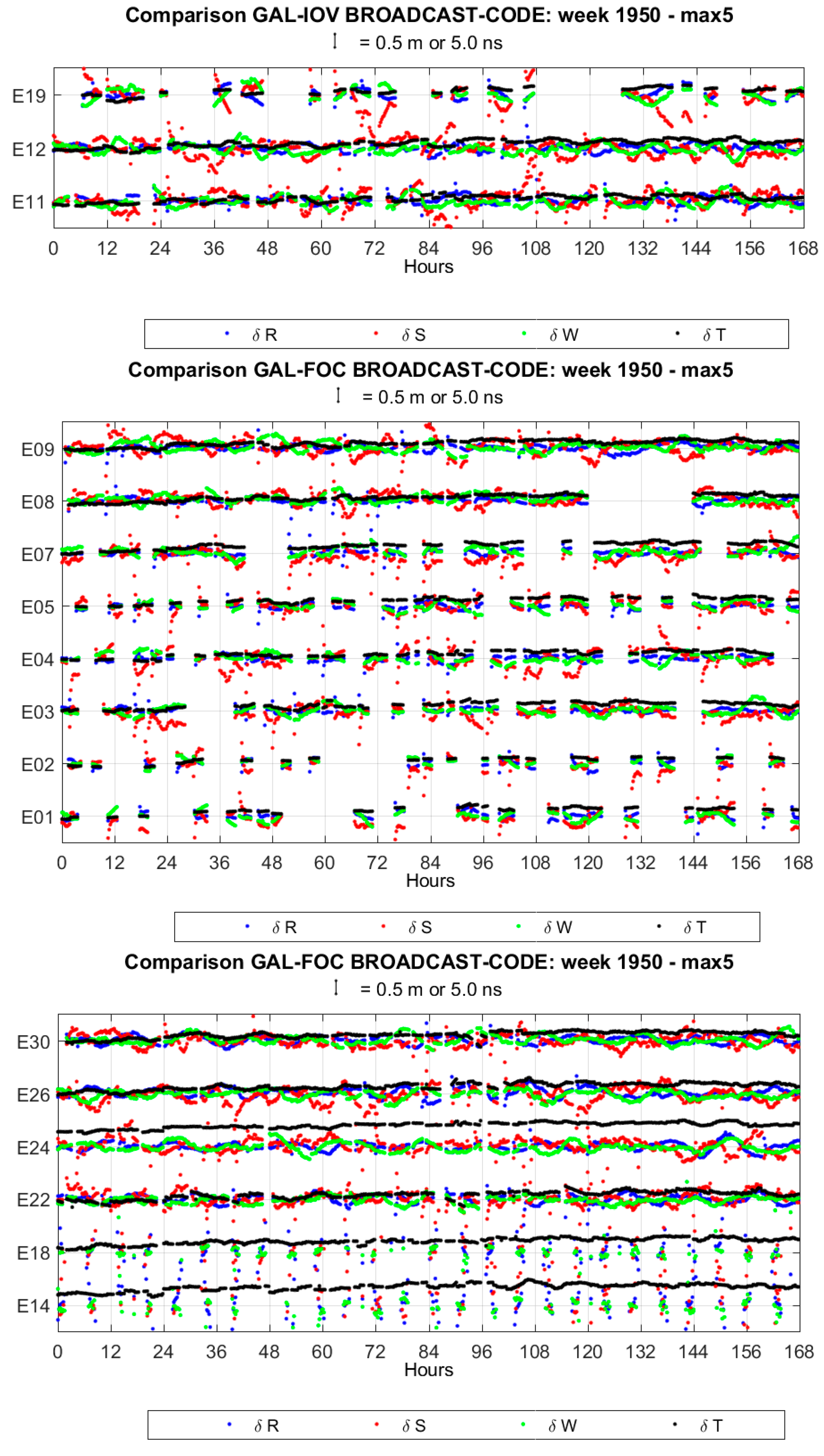
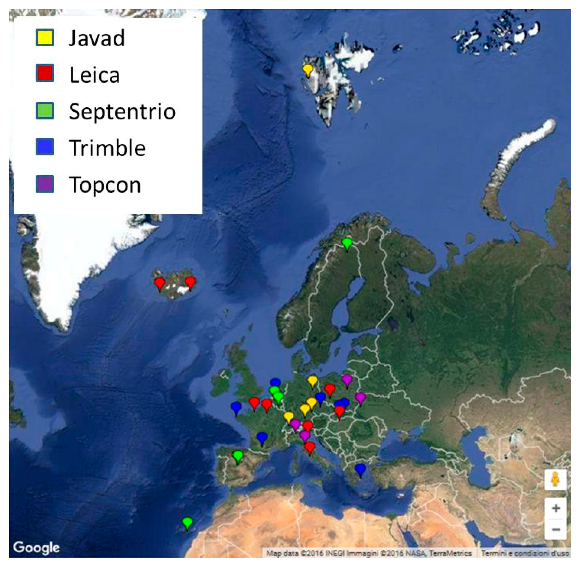
As part of the contribution of the University of Padova to the MGEX program [1] and to the activities of the MultiGNSS Working Group within [2], 31 European GNSS sites have been monitored since 2014 with five different receivers (Javad, Leica, Septentrio, Topcon, Trimble). The location of the sites is shown in Figure 1 and the equipment at each site is described in Table 1. Three issues which are critical for the interoperability of the different GNSS constellations are considered from the user point of view:

Figure 1.
Map view of monitored sites.

Table 1.
List of stations included in the analysis.
- Alignment of the spatial reference frame implied by the broadcast orbits to a common frame aligned to ITRF (International Terrestrial Reference Frame), such as the one implied by the preciseephemeris of CODE (Center for Orbit Determination in Europe) at the University of Bern.
- Offset among the time scales of different GNSS constellations: are the reference time scale of the various GNSSs synchronized among each other?
- Do different receivers measure different offsets? Does the receiver dependent offset change subject e.g., to a firmware update?
GPS, GLONASS, Galileo and BeiDou are the systems taken into account. For some receivers at higher latitude (e.g., KIRU, Kiruna, Sweden; WROC, Wroclaw, Poland; NYA2, Ny Alesund, Svalbard; DLF1, Delft, The Netherlands; GANP, Ganovce, Slovak Republic) QZSS data are also available. A Septentrio receiver has also delivered data from the Indian NAVIC (formerly IRNSS) constellation. SBAS data are received from satellites S27 and S28, both belonging to the Indian overlay system GAGAN (GPS Aided Geo Augmented Navigation) in geostationary orbits. No data usable for positioning are available from other SBAS systems.
This paper is organized in two parts. In the first part, the offset between broadcast reference frames and ITRF has been evaluated, together with a comparison between broadcast and precise orbits and clocks. This part is described in Section 2. The second part of the paper focuses on the misalignment of the time scales adopted by GNSSs, and is described in Section 3 and Section 4.
Montenbruck et al. [3] have carried out a similar analysis for the whole of 2013. In their study, they evaluate the signal-in-space ranging error (SISRE), which describes the error contributions due to broadcast orbits and clocks. They found that the GPS broadcast ephemerides show the best accuracy, with a RMS (Root Mean Square) orbit error of 0.18, 1.05 and 0.44 m in radial, along-track and cross-track directions respectively, and 2 ns as clock errors. For the other GNSS systems they found errors two to three times higher. The computed SISRE values confirm the better accuracy of GPS orbits compared to other GNSS’s, since the global average SISRE values are 0.7 ± 0.02 m (GPS), 1.5 ± 0.1 m (BeiDou), 1.6 ± 0.3 m (Galileo) and 1.9 ± 0.1 m (GLONASS). These results apply to data available in 2013. Since then the quality of the signals and orbits have considerably improved, and a re-evaluation of the whole issue is justified.
MATLAB-based multiGNSS software (The MathWorks, Inc., Natick, MA, USA) is used for this purpose [4], which allows the estimation at each epoch of the three receiver coordinates, one Tropospheric Zenith Delay and nGNSS receiver time offsets, where nGNSS is the number of tracked GNSS constellations. The latter unknowns are the sums of the receiver clock offset and the offset of the GNSS time scale relative to a common, interGNSS time scale [5]. Differentiation of such an offset relative to the GPS data yields, epochwise and for each receiver, estimates of the GNSS time offset to GPS. Comparing across different receivers it can be seen that such offsets can be biased relative to each other by as much as several tens of nanoseconds. The average of six Septentrio receivers was arbitrarily selected as reference to estimate the receiver biases relative to the average Septentrio. For a given receiver brand, the bias relative to Septentrio for the various GNSS is very repeatable, with a few exceptions. It turns out that updating the firmware often affects the GNSS-dependent receiver bias. There are however examples of changes of the receiver-dependent bias which are uncorrelated with a firmware update. A table of “individual” calibrations, for each receiver and each GNSS time offset is presented.
2. Quality Check of Broadcast Orbits
To study the accuracy of the broadcast orbits relative to the precise orbits provided by CODE [6] SP3 (Extended Standard Product 3 Orbit Format), the alignment of the reference systems adopted by broadcast orbits with respect to that provided by precise orbits is analyzed. The reference frames adopted by the several GNSSs in the broadcast ephemeris are different from each other, namely WGS84 (GPS), PZ-90.11 (GLONASS), GTRF (Galileo) and CGCS2000 (BeiDou), whereas the reference frame adopted by precise orbits is typically unique. According to [7,8], current GLONASS broadcast ephemerides and all those since 31 December 2013 should be referred to PZ-90.11 as it is aligned to ITRF at millimeter level. The reference frame adopted by CODE during week 1950 is IGS14.
Broadcast and precise orbits are referred to different points of space vehicles: the antenna phase center (APC) and the center of mass (CoM), respectively. The relative distance of APC to CoM is the antenna phase offset (APO). Montenbruck et al. [3] decided not to apply any reference frame transformation in their comparative analysis. They inferred the APO from the comparison between broadcast and precise orbits except for BeiDou, for which they assumed that the broadcast ephemeris is referred to the CoM.
In this section the coordinate differences in the RSW (radial, along-track, cross-track) reference system (Figure 2) are also analyzed and computed on the post-fit residuals of the seven-parameter Helmert transformation [9] between broadcast and precise ephemeris, for each day and satellite of the four GNSSs: GPS, GLONASS, Galileo, BeiDou. To achieve this goal, the Bernese software [10] was used with a maximum threshold of 5 m as a condition for coordinate rejection.
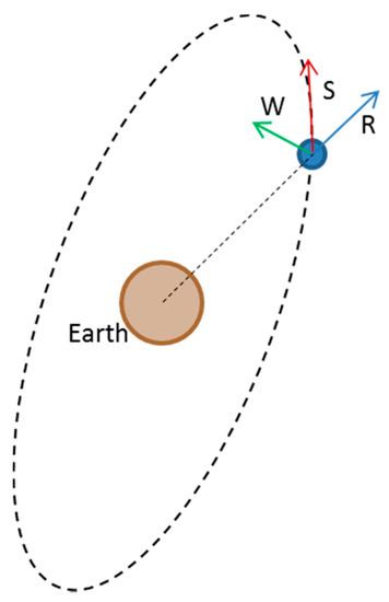
Figure 2.
RSW reference system: radial (R), along-track (S) and cross-track (W).
2.1. Comparison of Reference Systems
The study focuses on GPS week 1950, i.e., from 21 May 2017 to 27 May 2017. For each day a set of Helmert parameters are obtained, which define the transformation from precise to broadcast reference systems, and consist of three translations (Tx, Ty, Tz), three rotations (Rx, Ry, Rz) and one scaling factor (k) according to Equation (1).
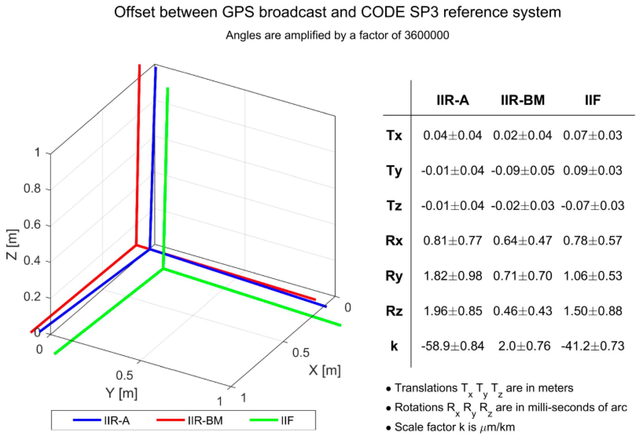
The weekly average values of each Helmert parameter has been computed. With these mean values the broadcast reference systems relative to precise reference system have been represented. Figure 3, Figure 4, Figure 5 and Figure 6 show the rotations magnified in order to be visible (milliarcsecs are treated as degrees). The figure also contains a table with the sets of mean Helmert parameters and their standard deviation, for each block of satellites. Translations are measured in meters, rotations in milliarcsec and the scaling factor is expressed in μm/km (1 μm = 10−6 m).
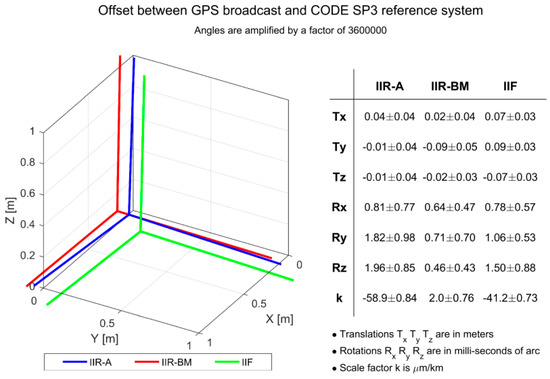
Figure 3.
Representation of the offsets between the three GPS blocks (IIR-A, IIR-B/M, IIF) broadcast and precise reference system of CODE SP3.
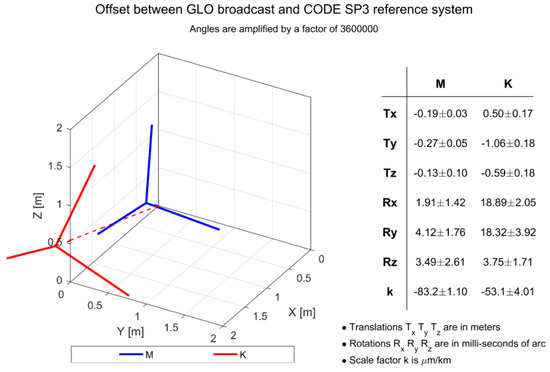
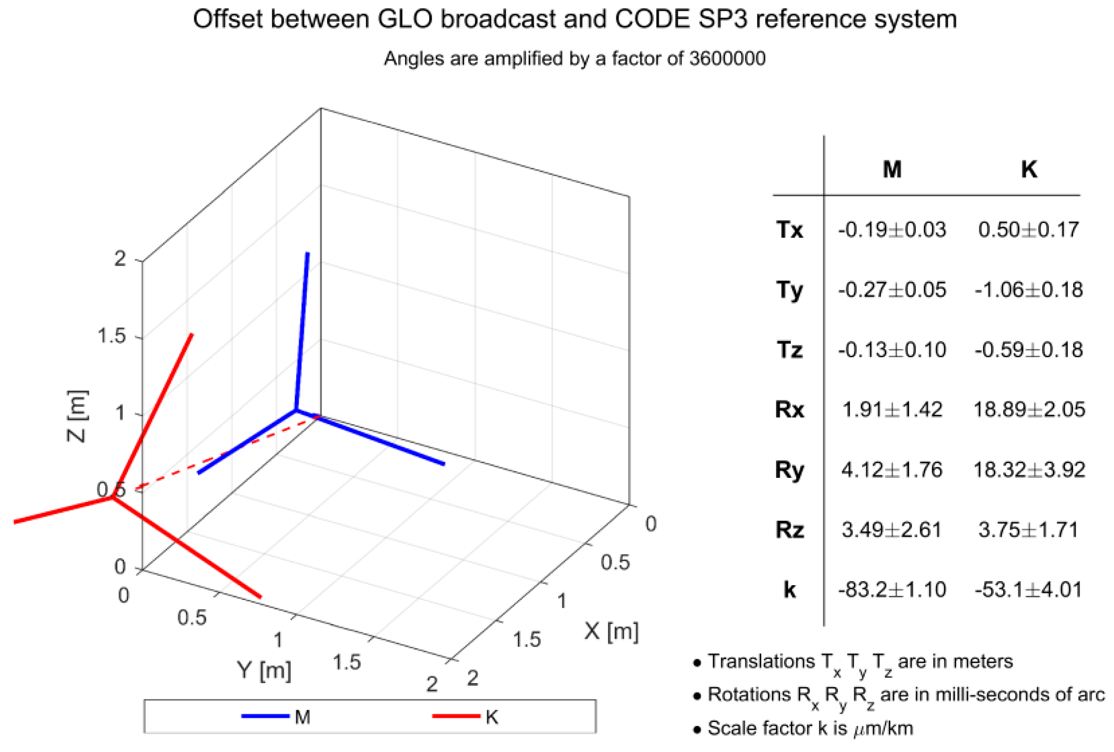
Figure 4.
Representation of the offsets between the two GLONASS blocks (M, K) broadcast and precise reference system of CODE SP3.

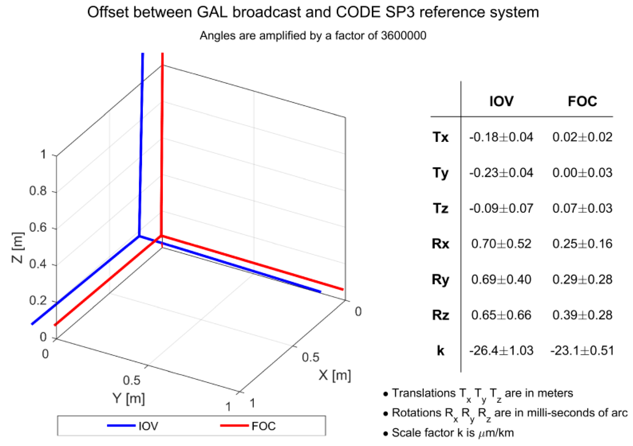
Figure 5.
Representation of the offsets between Galileo (IOV, FOC) broadcast and precise reference system of CODE SP3.

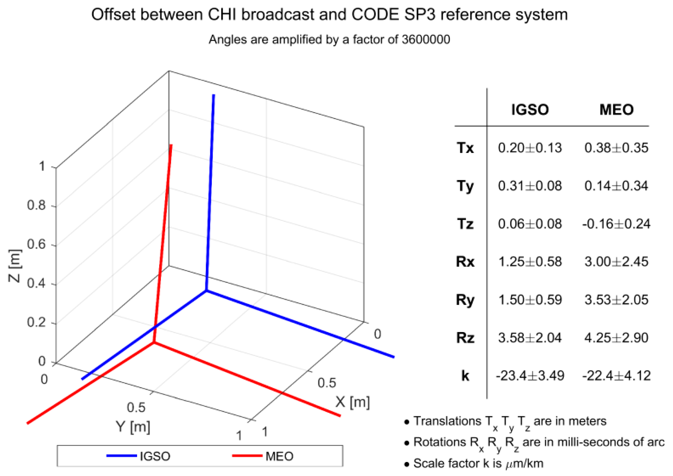
Figure 6.
Representation of the offsets between BeiDou broadcast (IGSO, MEO) and precise reference system of CODE SP3.
Precise orbits refer to CoM whereas broadcast orbits refer to APC. The relative distance between APC and CoM is the APO (Antenna Phase Offset). Among the three (x, y, z) APO components, the z component, which correspond to the boresight direction, is the prevalent one. Since APO is constant, the satellite orbits described by CoM and APC differ mainly by the constant offset given by the boresight component of APO, which is oriented in radial direction. So we assume that APO is absorbed by the scale factor of Helmert transformation.
For GPS and Galileo FOC (Full Operational Capability) satellites, the reference systems adopted by broadcast orbits are quite similar to those provided by precise orbits: the translation of the origin is less than 0.10 m and rotations are less than 2 milliarcsec. For Galileo IOV (In Orbit Validation), GLONASS and BeiDou higher differences are apparent. The Galileo IOV broadcast reference frame is offset to ITRF by at most 0.23 ± 0.04 m in Y (Figure 5).
The GLONASS M broadcast reference frame is offset to ITRF by at most 0.27 ± 0.05 m in Y and the maximum rotation is 4 ± 2 milliarcsec of arc about Y. The GLONASS K broadcast reference frame is offset to ITRF by at most 1.06 ± 0.18 m in Y and the maximum rotation is 19 ± 2 milliarcsec about X (Figure 4).
The BeiDou IGSO broadcast reference frame is offset to ITRF by at most 0.31 ± 0.08 m in Y and the maximum rotation is 3.6 ± 2.0 milliarcsec about Z (Figure 6). For BeiDou MEO satellites we find Helmert parameters of the same order of magnitude of those found for IGSO satellites, but with a higher uncertainty. This margin of error is probably due to the limited number of available satellites (only three). The BeiDou MEO broadcast reference frame is offset to ITRF by at most 0.38 ± 0.35 m in X and the maximum rotation is 4.3 ± 2.9 milliarcsec about Z (Figure 6).
2.2. RSW Components of Coordinate Differences and Clock Differences
Coordinate differences of broadcast vs. precise ephemeris of GPS are generally continuous. There are however occasional discontinuities, which affect mostly the along-track components. The coordinate differences in the radial and cross-track components may have an oscillatory pattern with a period of about 12 h. The average values of standard deviations are 0.15, 0.71, 0.34 m and 1.1 ns for the radial, along-track, cross-track and clock component, respectively.
As to the satellite clocks, it is found that all satellites are equipped with atomic rubidium clocks, except G08 and G24, which are equipped with cesium atomic clocks and belong to block IIF. The average values of clock differences range between −3.4 and 2.0 ns.
The magnitude of discontinuities is up to 0.3, 1.5, 0.2 m and 1 ns for the radial, along-track, out-of-plane and clock component, respectively. Mean values and standard deviations of coordinates and clock differences for each satellite are reported in Table 2. The complete time series of coordinates and clock differences for all GPS satellites are shown in Figure A1.
Table 2.
GPS mean values and standard deviations of coordinates and clock differences.
GLONASS coordinate and clock differences show an oscillating trend, with a period of about 12 h, and discontinuities, which affect mostly the along-track and clock components. The average values of standard deviations are 0.48, 1.35, 0.74 m and 5.6 ns for the radial, along-track, cross-track and clock component, respectively. Average values of clock differences are different from one satellite to another, varying from −20 to 24 ns. The magnitude of discontinuities is up to 0.3, 3.0, 0.3 m and 8 ns for the radial, along-track, out-of-plane and clock component, respectively.
Mean values and standard deviations of coordinates and clock differences for each satellite are reported in Table 3. The complete time series of coordinates and clock differences for all GLONASS satellites are shown in Figure A2.
Table 3.
GLONASS mean values and standard deviations of coordinates and clock differences.
BeiDou coordinate and clock differences show discontinuities, which affect mostly the along-track, especially for Medium Earth Orbit (MEO) satellites (C11, C12, C14), and clock components. Furthermore coordinate differences show an oscillating trend, with a period of about 12 h for MEO satellites and about a whole day for the other satellites (Inclined Geosynchronous Satellite Orbit—IGSO). The average values of standard deviations are 0.43, 0.81, 0.63 m and 2.3 ns for the radial, along-track, cross-track and clock component, respectively (except clock RMS of C11, for which a higher standard deviation is found, about 27 ns, due to two large discontinuities). Average values of clock differences are different from one satellite to another, varying from 56 ns to 122 ns. The magnitude of discontinuities is up to 0.3, 1 (IGSO) or 3 (MEO), 0.3 m and 5 ns for the radial, along-track, cross-track and clock component, respectively.
Mean values and standard deviations of coordinates and clock differences for each satellite are reported in Table 4. The complete time series of coordinates and clock differences for all BeiDou satellites are shown in Figure A3.
Table 4.
BeiDou mean values and standard deviations of coordinates and clock differences.
For Galileo, it is important to remember that three types of ephemeris are available: I/NAV E1-B, F/NAV E5a and I/NAV E5b. I/NAV E1-B ephemeris has been chosen because this type of ephemeris is updated more frequently in the timeframe considered. Referring to Galileo ICD (Interface Control Document) [11], I/NAV blocks with Health Status equal to 1 (Signal out of service) have been rejected and others accepted. Of the 17 satellites, 11 are found to have a SV health value of 0, which means Data Validity Status = “Navigation Data Valid” and Health status = “Signal OK”. For the other six satellites the same value is 455, which means Data Validity Status = “Working without guarantee” and Health status = “Signal Component currently in Test”. These satellites are the last four launched on 17 November 2016 (E03, E04, E05, E07) and the two launched on 22 August 2014 (E14, E18) into non nominal elliptical orbit [12]. The week analyzed is later than the epochs of orbit circularization, which were concluded in December 2014 and March 2015, respectively.
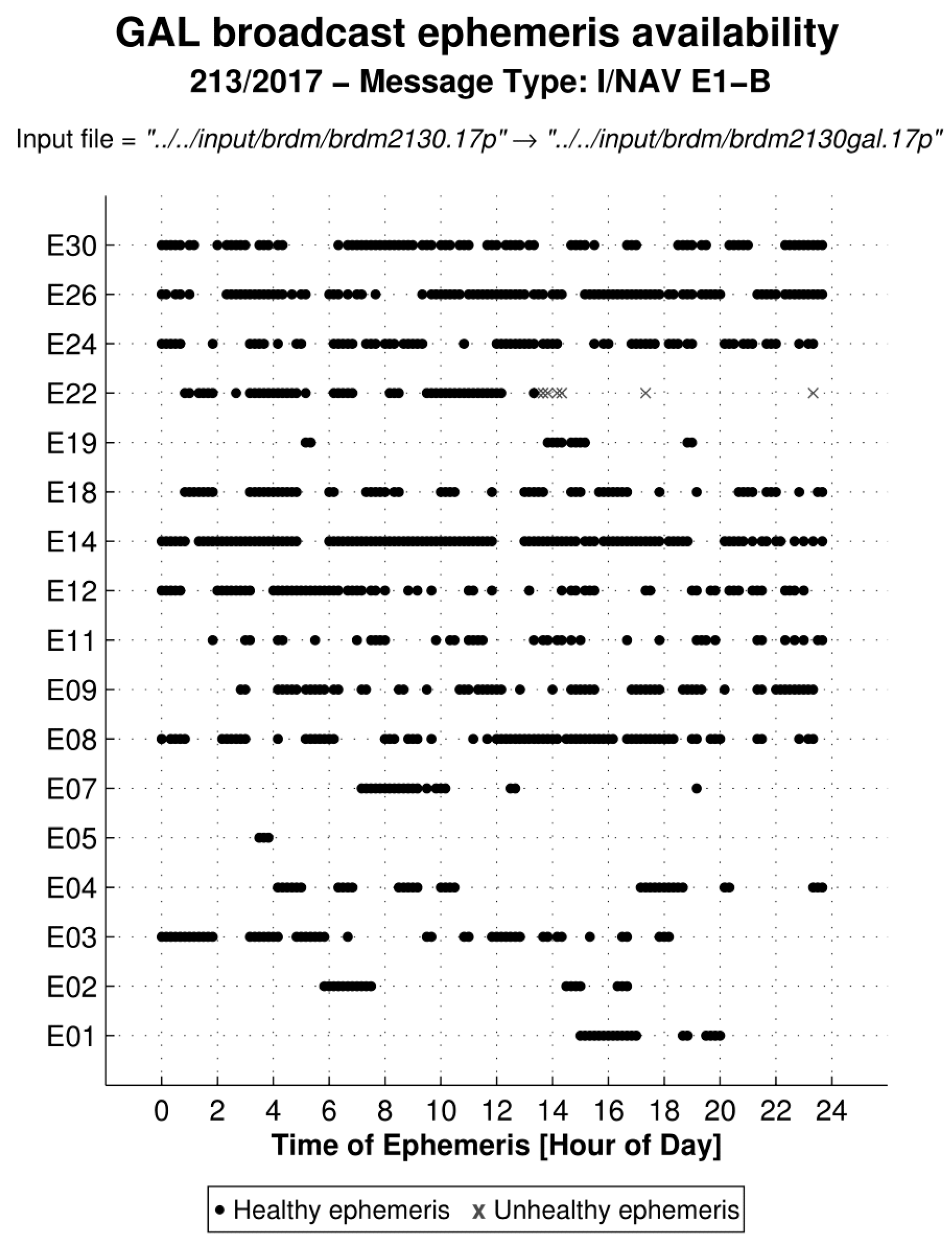
For Galileo, gaps have been found in the spacing between I/NAV ephemeris blocks larger than the validity period of the ephemeris block, i.e., ±3600 s. This prevents the computation of satellite coordinates and clock in the gaps. The availability of broadcast ephemeris is shown in Figure 7, where each block of healthy ephemeris is plotted with a circular black marker and each block of unhealthy ephemeris is plotted with a cross-shaped gray marker. In the studied days all the ephemeris blocks were set to healthy. In the periods of continuity of validity of ephemeris, it is possible to notice discontinuities in satellite coordinates (mostly in the along-track component) and clock.
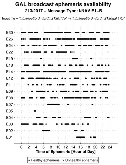
Figure 7.
Availability of Galileo I/NAV-E1-B broadcast ephemeris on day 1 August 2017.
For Galileo, the coordinate differences show an oscillating trend with a period of about 12 h. The average values of standard deviations are 0.14, 0.29, 0.16 m and 1.3 ns for the radial, along-track, cross-track and clock component, respectively. The average values of clock differences range between 0.7 and 7.8 ns. The magnitude of discontinuities is up to 0.2, 1.0, 0.3 m and 2 ns for the radial, along-track, cross-track and clock component, respectively.
E14 and E18 show scattered coordinate differences with very large (>5 m) values, so about 75% of coordinates are rejected by Bernese and not considered in the estimating of Helmert parameters. Their clock differences show an offset of about 4–8 ns, with the same standard deviation of the other satellites.
Mean values and standard deviations of coordinates and clock differences for each satellite are reported in Table 5. The coordinate and clock accuracy of In-Orbit Validation (IOV) satellites is consistent with that of the Full Operational Capability (FOC) satellites. Both generations of satellites are equipped with passive hydrogen maser (PHM) clocks. The complete time series of coordinates and clock differences for all Galileo satellites are shown in Figure A4.
Table 5.
Galileo mean values and standard deviations of coordinates and clock differences.
3. Data Used and Adopted Model of the Pseudorange
RINEX (Receiver Independent Exchange Format) 3.x [13] observation data was used for all receivers except Topcon, for which the provided RINEX 2.x files are converted to RINEX 3.x with the utility gfzrnx of the German Research Centre for Geosciences (GFZ) [14]. As to the orbits, satellite clocks and other ancillary data (e.g., quality flags), broadcast ephemeris in RINEX format downloaded from the MGEX FTP servers was used [1].
Several codes are available in the carriers at several frequencies, for the different GNSS constellations. The well-known “iono-free” linear combination of dual frequency code observations was used in order to remove first order ionospheric delay [9]. Table 6 summarizes the GNSS specific frequency bands and observation codes. The GPS broadcast clock model refers to iono-free combination of precise codes, i.e., C1W-C2W. We decided to analyze the combination C1C-C2W because about half of the stations (more precisely all the Leica and Trimble stations) do not track C1W. The error introduced using C1C in place of C1W depends on GPS satellite and varies between about −1 and 1 m. This means about ±3 nanoseconds which is within the accepted tolerance. For GLONASS, the k factor varies from −7 to +6 according to the satellite [15]: such information is provided in the header of the observation RINEX file. For Galileo the I/NAV combination of codes and the related navigation message is used [11].
Table 6.
Frequencies and observation codes used.
The model of the pseudorange p(t) is described in Equations (2)–(6). In Equation (2) the effect of the Differential Code Bias (DCB) as listed in files provided by CODE has been ignored. For GPS the DCBs are up ±2 nanoseconds which is within our error budget. For GLONASS the DCBs are station-dependent and the estimates are provided only for a small subset of stations, for the other constellations no DCBs are provided (ftp://igs.bkg.bund.de/IGS/products/mgex/). Table 7 contains the explanation of the variables. The matrix of partial derivatives is shown in Equation (7), where seven GNSS are considered: GPS, GLONASS, Galileo, BeiDou, QZSS, NAVIC and GAGAN. The term ρ indicates the geometric range between satellite and receiver.
Table 7.
Explanation of symbols and variables used in Equations (2)–(6).
In Equation (8) y is defined as the column vector of observed minus computed: each element of y is the difference between iono-free linear combination of pseudoranges and the right side of Equation (2). The number of elements of y is equal to the number of satellites in view.
The column vector of the solution, denoted as x, is the solution of the normal equations expressed by Equation (8). The vector x consists of three coordinates, n terms TSCX + dTRec, where n is the number of GNSS’s considered, and one TZD (Tropospheric Zenith Delay). The explicit form of the solution is given in Equation (9). Term TSCX is a GNSS-specific Time System Correction, which is dependent on the GNSS but independent of the receiver. Term dTRec is the receiver clock offset, which is independent of the GNSS. However we will see later that different receivers measure different TSCX implying receiver biases which are dependent both on the receiver and the GNSS [16]. To monitor the GNSS specific time offset it is convenient to take TSCG as the reference time scale and evaluate the difference (TSCX + dTRec) − (TSCG + dTRec), with X referring to all the GNSS’s different from GPS [17]. In such a way we obtain the sum of the system specific time offset relative to GPS and the receiver hardware inter-system bias (ISB) [17,18,19]. Table 8 lists these specific variables.
Table 8.
Definition of Time Offsets.
4. Results of the Positioning Analyses
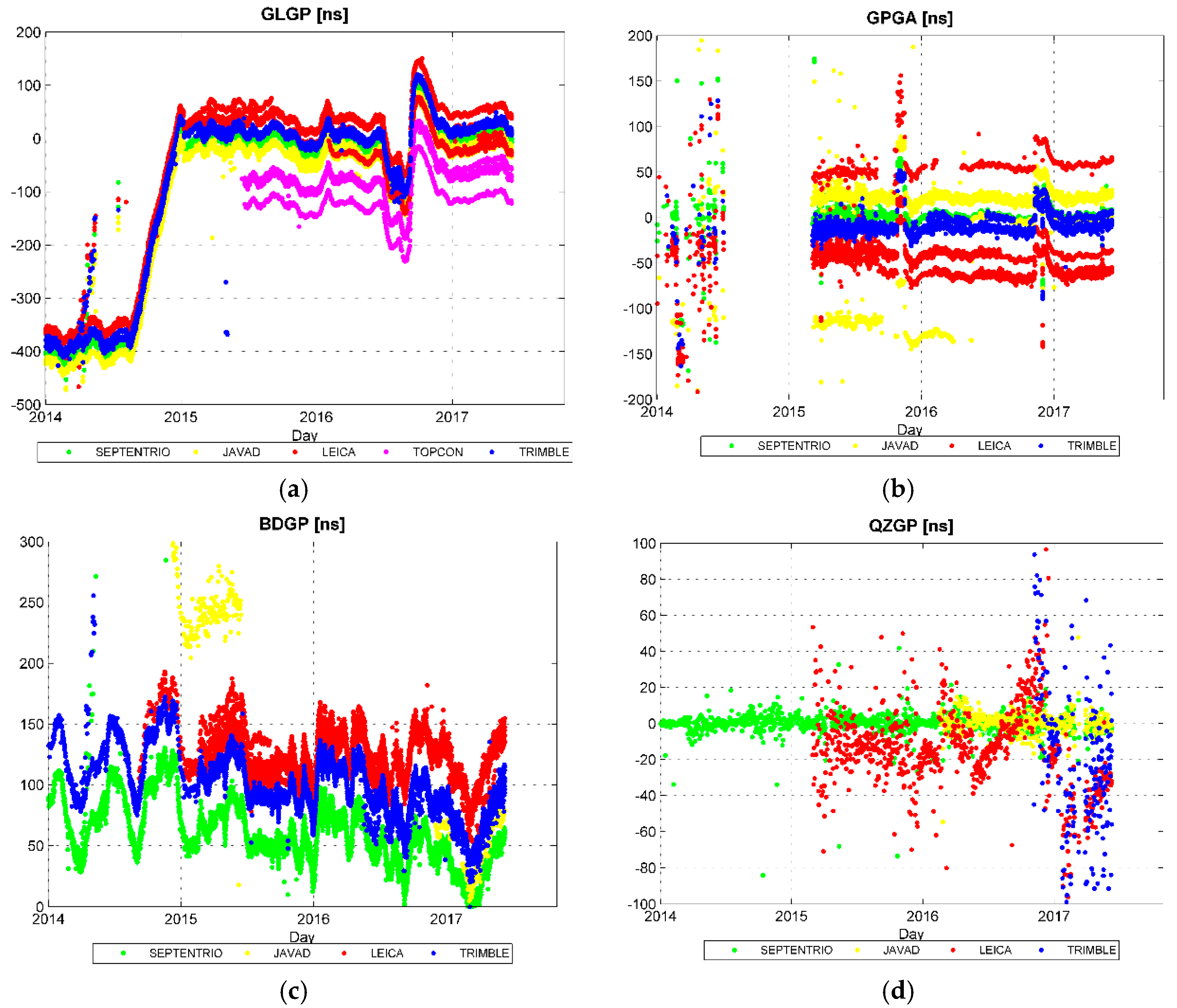
Daily analysis has been performed on the 31 stations listed in Table 1 and shown in Figure 1 starting from 1 January 2014 and is currently ongoing. Figure 8 shows the time series of GLGP, GPGA, BDGP and QZGP, distinguishing between the five types of receiver.
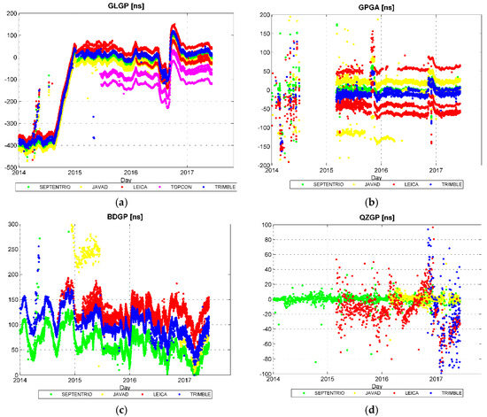
Figure 8.
Time series since 1 January 2014 of offsets of the GLONASS (a), Galileo (b), BeiDou (c) and QZSS (d) time scales relative to GPS.
In the GLGP time series a very large misalignment of about −400 ns from the beginning of the analyses until mid-August 2014 can be seen. Then a re-aligning procedure started and was completed at the end of 2014. From the beginning of 2015 the GLONASS time scale is generally kept aligned with GPS, but several short-term variations with amplitudes ranging from tens to about one hundred ns are evident. The largest variation observed happened from July to December of 2016, and has a sinusoidal shape with an amplitude of about 100 ns.
BDGP varies continuously, with an oscillating trend and amplitude of about 70 ns. Furthermore the oscillations have a positive mean, which results in an average positive offset of the BeiDou time scale with respect to GPS. Considering a time series of more than three years it is possible to notice a slow trend toward zero, but it is not clear if this long-term variation is effectively a re-alignment procedure of the BeiDou time scale to GPS.
GPGA is aligned with GPS, since the time offset series are almost constant in time and centered to zero. Two sudden variations took place in November 2015 and November–December 2016, measuring about 60 and 30 ns, respectively.
The QZGP system time is aligned with GPS, but unfortunately for this system data from only five of the 31 stations is available. Among these five stations, Leica and Trimble receivers show higher scattered results compared to those of Septentrio and Javad, despite the global average value is very close to zero. It is important to notice that until June of 2017 there was only one satellite belonging to QZSS, so QZGP actually represents the time offset between this single satellite and GPS.
4.1. Differential Time Offset
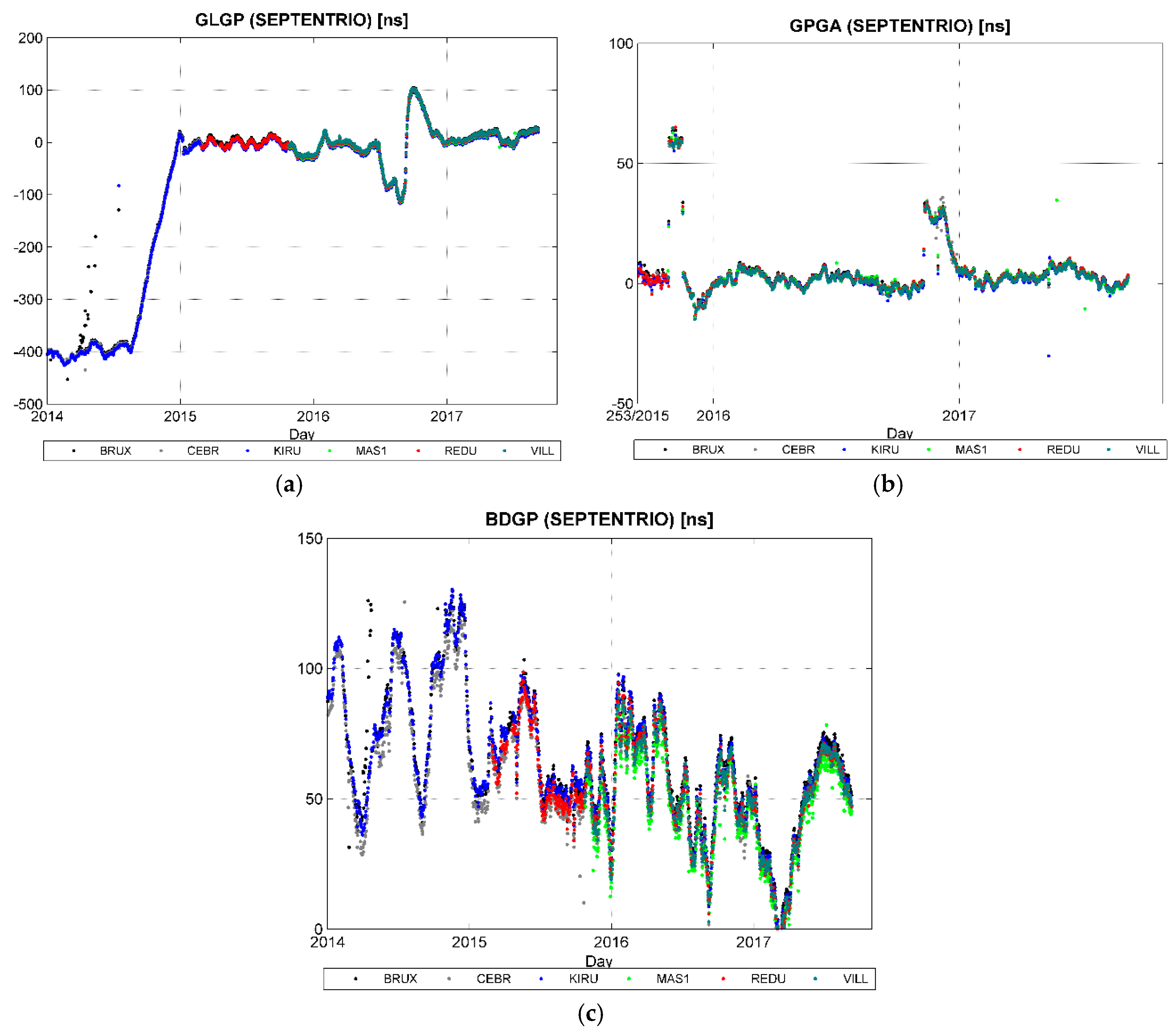
A receiver-dependent bias is clearly visible in Figure 8, as previously noted by [17,20,21]. In order to better investigate this receiver dependent bias, the time series relative to the mean values of Septentrio stations have been differentiated. The choice of Septentrio is due to the observation that these stations show very similar values: for each day the RMS is generally lower than 3 ns. Figure 9 shows the time series of GLGP, GPGA and BDGP obtained for individual Septentrio stations. The QZGP time series is not shown since there is only one station among the six Septentrio stations which tracks this constellation.
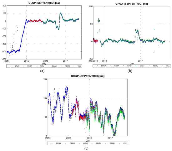
Figure 9.
Time series since 1 January 2014 of offsets of the GLONASS (a), Galileo (b) and BeiDou (c) time scales of Septentrio stations relative to GPS.
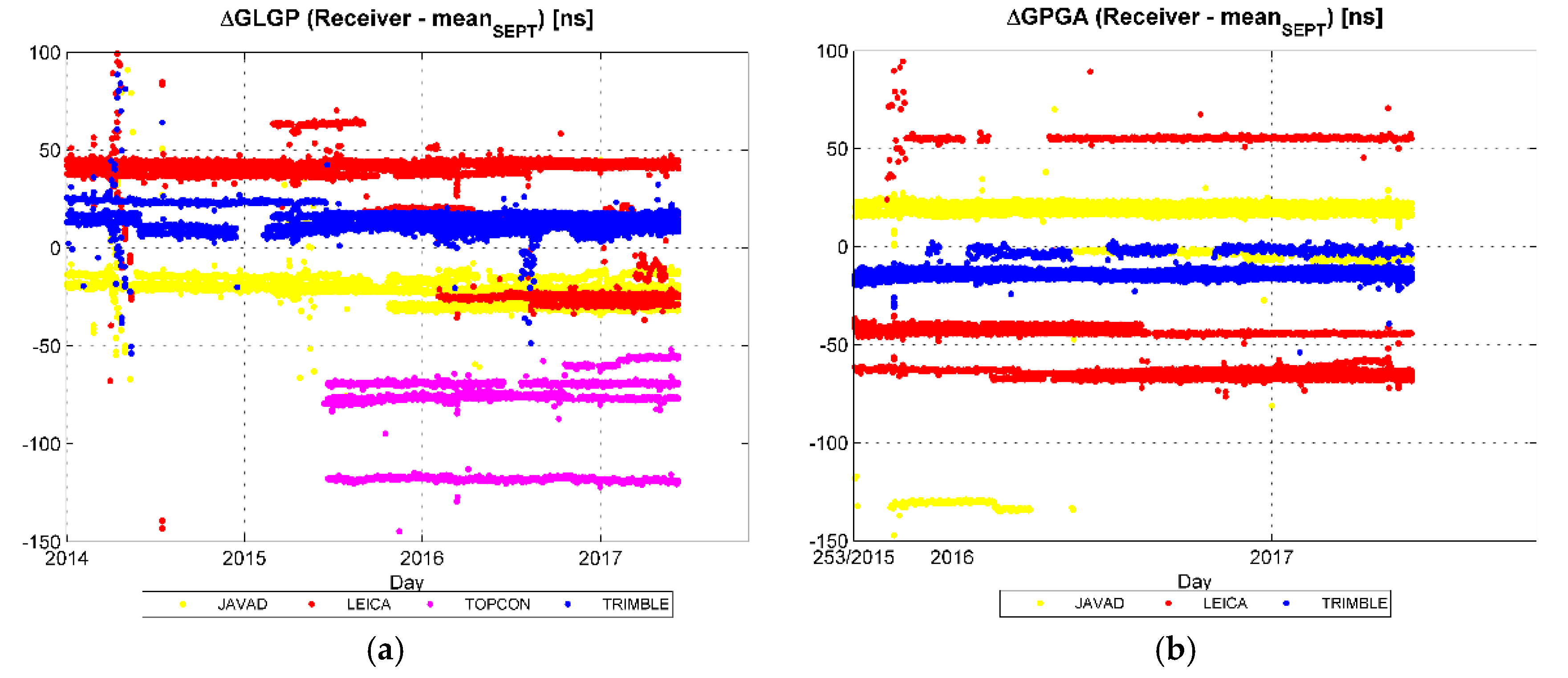
The graph of GPGA in Figure 10 starts from 9 October 2015 due to the high scatter observed before this date. From these graphs the receiver dependent bias can be monitored. It is worth noting that for a given receiver type, some stations show similar time offsets, so their time series are quite superimposed, whereas other stations show different values and this difference seems to be constant in time. For example in Figure 10a it is possible to notice that the Trimble and Javad receivers have very similar time offsets, whereas Leica and Topcon show a relative bias up to tens of nanoseconds.
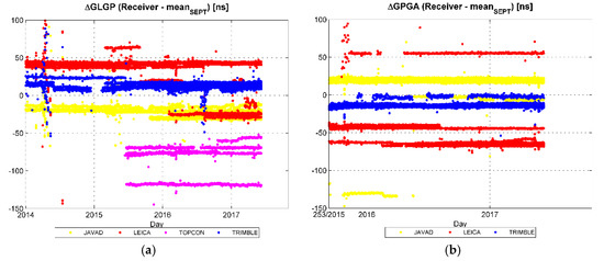
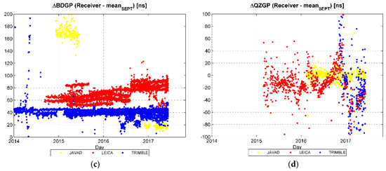
Figure 10.
Time series since 1 January 2014 of offsets of GLGP (a), GPGA (b), BDGP (c) and QZGP (d) differentiated relative to Septentrio.
In Figure 10a a discontinuity of several Leica stations from about 40 ns to about −25 ns in the first half of 2016 is evident. These stations are: CAEN, M0SE, MLVL, PADO, REYK (Table 1). Taking into account the station logsheets it was possible to identify an exact connection between some of the discontinuities in the time offset series and receivers’ firmware updates. For example, considering the five Leica stations mentioned above, the correspondence between the discontinuity in the GLGP time offset and the update of receivers firmware for M0SE, PADO and REYK could be observed.
4.2. Analysis of Other Constellations: NAVIC and GAGAN
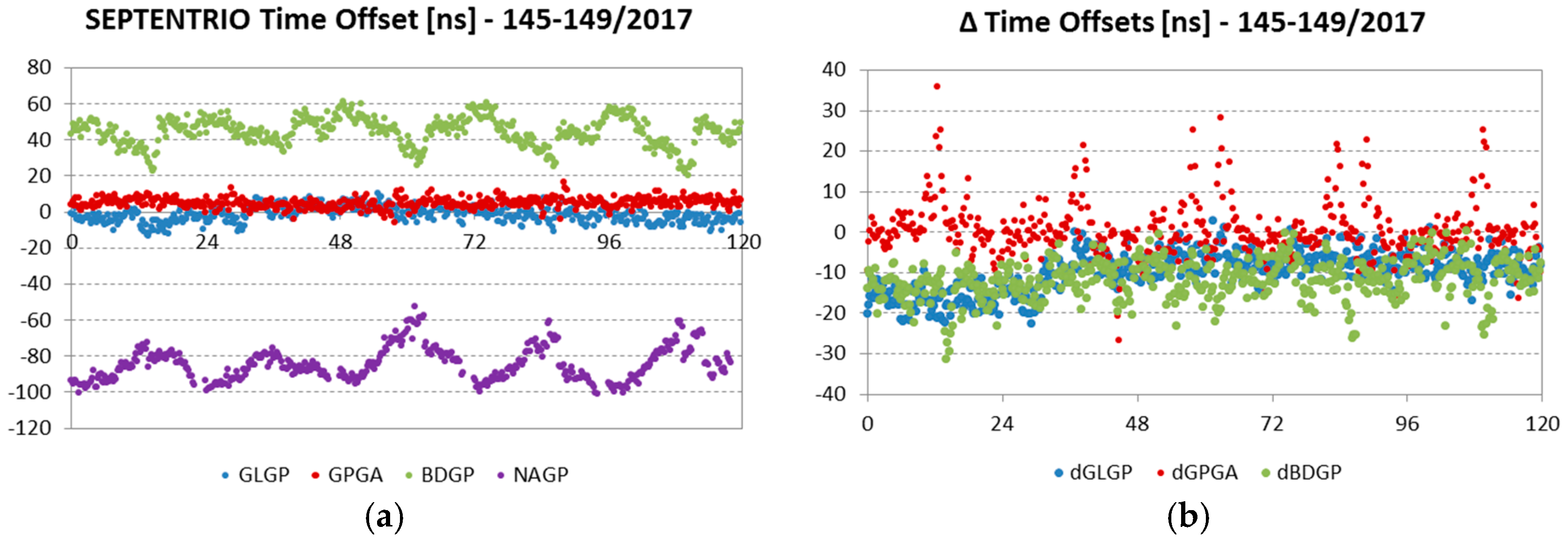
The multiGNSS software [4] has the capability to analyze the observations from NAVIC and SBAS, in addition to GPS, GLONASS, Galileo, BeiDou and QZSS. Septentrio has kindly made available RINEX data of days 25–29 May 2017 from their station located in Brussels (not listed in Table 1). This gave the opportunity to analyze the NAVIC time offsets for these five days. This station is equipped with a POLARX5 5.11 receiver, referred to as SEPT hereafter. It is worth noting that the observation data of the NAVIC satellites are available for the L5 carrier only, for which NAVIC has been processed in single frequency.
Figure 11a shows the results. The offset of NAVIC time scale relative to GPS is colored in purple. The NAVIC time offset is characterized by a daily variation which can reach 20 ns. Across the five days, NAGP seems to be quite constant, with a mean value of about −85 ± 9 ns.

Figure 11.
Time offsets of Septentrio station. (a) Time offsets of GLONASS, Galileo, BeiDou and NAVIC (purple) relative to GPS; (b) GLGP, GPGA and BDGP relative to the other Septentrio stations.
Figure 11b shows the time offsets of SEPT differentiated to the other six Septentrio stations currently analyzed. GLGP and BDGP are smaller than those of other stations, whereas GPGA is very close. More in detail, the difference of GLGP varies suddenly from −16.5 to −7.5 ns on 26 May 2017, with a standard deviation of 3 ns. The GPGA of six Septentrio stations show spikes at 12:00 and 24:00 of each day, whereas SEPT does not. Otherwise the alignment is within 1 ns. The difference of BDGP is almost constant, with a mean value of about −12.5 ± 5 ns.
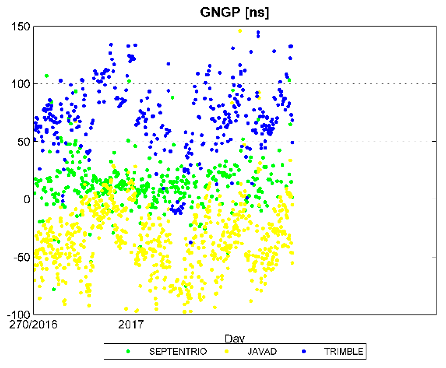
For SBAS data for satellites S27 and S28, both belonging to the Indian overlay system GAGAN in geostationary orbits have been used. These satellites are tracked by seven stations (DLF1, KIRU, REDU, TLSE, WTZ3, WTZZ, ZIMJ). The GAGAN data were analyzed only from 25 September 2016, so as yet not enough results are available to perform a calibration of the GAGAN time offset like those described in the previous paragraph.
Figure 12 shows the results obtained. Trimble stations give higher offsets, Javad stations give lower offsets and Septentrio stations give offsets comprised of those from the previous two receiver types. Septentrio GNGP seems to be quite constant in time, whereas for Trimble and Javad higher variations are observed.
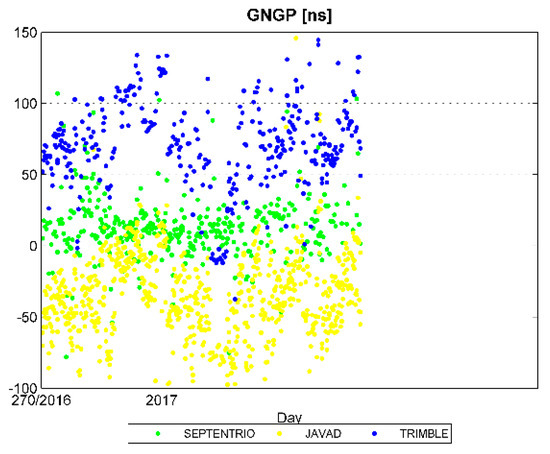
Figure 12.
Time series since 25 September 2016 of offset of the GAGAN time scale relative to GPS.
5. Discussion
The observed correspondences between the discontinuities in the time offset series and receiver firmware updates suggest a relationship between the two events. In order to better investigate this relationship, the information about receiver set up and the time offsets relative to Septentrio have been summarized in Table 9. In this table the marker name of a station is followed by a lowercase letter if at least one discontinuity in time offset series is observed. The lowercase letter indicates a continuity period of time offsets, so a station name associated with the same letter has the same time offsets.
Table 9.
Calibration of station’s time offsets relative to Septentrio.
For each station every row corresponds to a new receiver set up or new time offsets relative to Septentrio, or both the events: in this case the discontinuity of time offsets corresponds to an update of receiver set up. These correspondences are highlighted by using a bold font.
A total number of 19 discontinuities have been identified. Among these, 11 are connected to receiver updates and six are due to unknown causes. Two of the 11 discontinuities connected to a receiver update involve also the antenna: COMOc and GANPc, as it can be noticed in Table 1. The other two discontinuities are linked to changes in antenna configuration: TLSEb shows a discontinuity on 11 March 2016, when the alignment from Nord was changed from 0 to −140 degrees, WTZZb shows a discontinuity on 13 July 2015, when the ARP (Antenna Reference Point) Up was changed from 0.045 to 0.284 m.
In Table 9 there are 92 receiver firmware updates, only 11 of these are connected with a discontinuity in time offset. So most of the receiver updates do not imply a discontinuity in time offset. Conversely more than half of the discontinuities in time offsets are connected to an update of receiver firmware. For these reasons it is necessary to keep monitoring both the configuration changes of receivers and the time series of time offsets.
6. Conclusions
In the present work a study of the accuracy of broadcast orbits has been presented, taking into account a time span of one week. In this phase, the offset between broadcast reference frames and ITRF has been evaluated, for homogeneous blocks of satellites. The results of an analysis carried out starting from 1 January 2014 and still active were presented, aimed at the evaluation of the misalignment between timescales of the various GNSS’s. In the next sections the main results obtained are summarized and discussed.
6.1. Reference Frames
Reference frames adopted by GPS and Galileo FOC broadcast orbits, in the week taken into account, are aligned with ITRF since the translation of the origin is less than 0.10 m and rotations are less than 2 milliarcsec. For Galileo IOV, GLONASS and BeiDou instead translations at dm-level and rotations higher than 4 milliarcsec have been found.
The Galileo IOV broadcast reference frame is offset to ITRF by at most 0.23 ± 0.04 m in Y.
The GLONASS M broadcast reference frame is offset to ITRF by at most 0.27 ± 0.05 m in Y and the maximum rotation is 4 ± 2 milliarcsec about Y. The GLONASS K broadcast reference frame is offset to ITRF by at most 1.06 ± 0.18 m in Y and the maximum rotation is 19 ± 2 milliarcsec about X.
The BeiDou IGSO broadcast reference frame is offset to ITRF by at most 0.31 ± 0.08 m in Y and the maximum rotation is 3.6 ± 2.0 milliarcsec about Z. BeiDou MEO broadcast reference frame is offset to ITRF by at most 0.38 ± 0.35 m in X and the maximum rotation is 4.3 ± 2.9 milliarcsec about Z.
6.2. Coordinates and Clock Comparison
In general coordinate and clock differences have been demonstrated to be discontinuous and show an oscillating trend with a period of about 12 h (except BeiDou IGSO satellites which have a period of about 24 h). The discontinuities affect mostly the along-track component, in which they are about 1 m for GPS, Galileo and BeiDou IGSO and up to 3 m for GLONASS and BeiDou MEO, and to a lesser extent the radial and cross-track components, in which they are at dm-level.
GPS and Galileo broadcast ephemeris are closer to the precise orbits than those of GLONASS and BeiDou: for GPS and Galileo the average values of RMS are about 0.15 m and 1 ns whereas for GLONASS the average RMSs are 0.48 m and 5.6 ns and for BeiDou 0.43 m and 2.2 ns.
6.3. GNSS’s Time Offsets
GLONASS time scale was misaligned with respect to GPS by about −400 ns until the summer of 2014, when an alignment procedure started, according to [8]. This procedure was completed at the beginning of 2015, so currently the GLONASS timescale is aligned with GPS. Despite this the alignment is not constant, and there may be non-predictable variations with amplitude up to 100 ns, like the one that happened in the second half of 2016.
BeiDou timescale is not aligned with GPS. The time offset vary continuously, with an oscillating trend and amplitude of about 70 ns. Furthermore it is not centered to zero, but it is always positive, although a slow trend of the average value to zero has been detected.
Galileo and QZSS time scales are aligned with GPS, although for Galileo two sudden variations, in November of 2015 and November–December of 2016, of about 60 and 30 ns, respectively, were noticed.
In addition to the previous constellation-specific considerations, for each time offset a receiver-dependent Inter System Bias (ISB) which could reach several tens of nanoseconds was evident. This bias tends to be almost constant in time, and so it could be calibrated. Since ISB is receiver-dependent, an upgrade of receiver firmware can change its amount and a new calibration is required.
The time offsets of 31 IGS/EUREF stations since 1 January 2014 were monitored. For each station, the potential discontinuities in time series of time offsets have been detected, and whenever possible the cause of discontinuity has been identified. Hence, for each continuity interval a relative-to-Septentrio calibration of time offsets has been evaluated.
Author Contributions
Luca Nicolini analyzed the data and wrote the paper; Alessandro Caporali conceived the model and supervised the work.
Conflicts of Interest
The authors declare no conflict of interest.
Appendix A
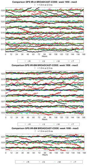
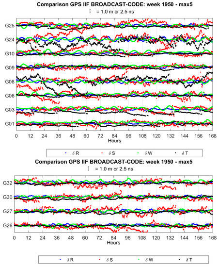
Figure A1.
GPS coordinates and clock differences. “max 5” refers to the maximum threshold of 5 m as a condition for coordinate rejection.
Figure A1.
GPS coordinates and clock differences. “max 5” refers to the maximum threshold of 5 m as a condition for coordinate rejection.

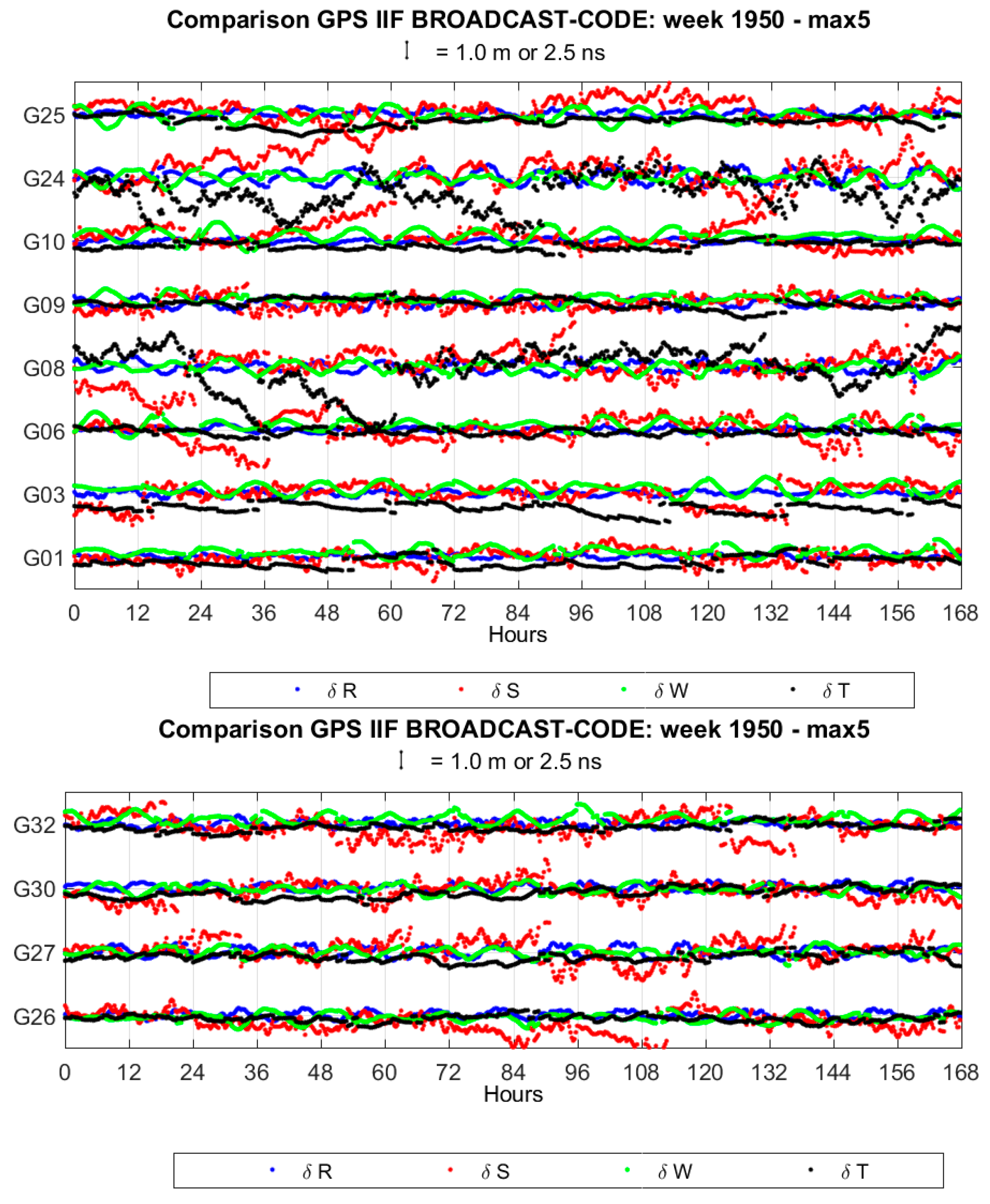
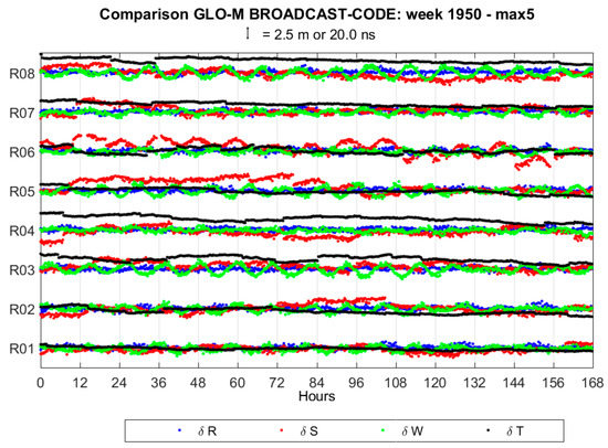
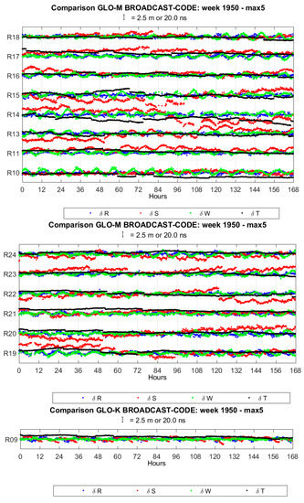
Figure A2.
GLONASS coordinates and clock differences. “max 5” refers to the maximum threshold of 5 m as a condition for coordinate rejection.
Figure A2.
GLONASS coordinates and clock differences. “max 5” refers to the maximum threshold of 5 m as a condition for coordinate rejection.
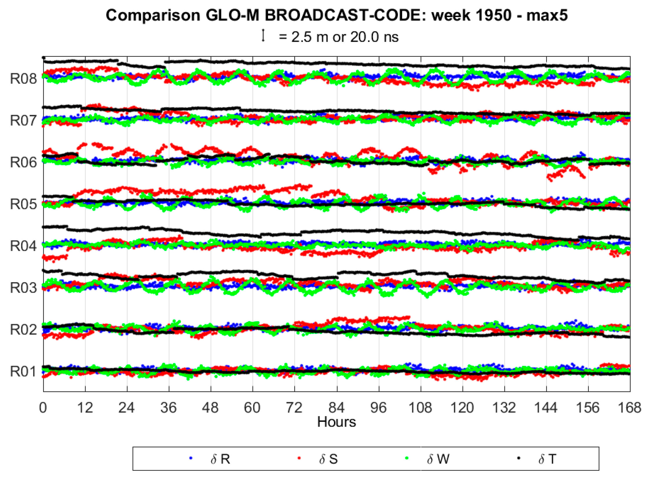


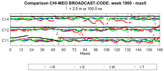
Figure A3.
BeiDou coordinates and clock differences. “max 5” refers to the maximum threshold of 5 m as a condition for coordinate rejection.
Figure A3.
BeiDou coordinates and clock differences. “max 5” refers to the maximum threshold of 5 m as a condition for coordinate rejection.
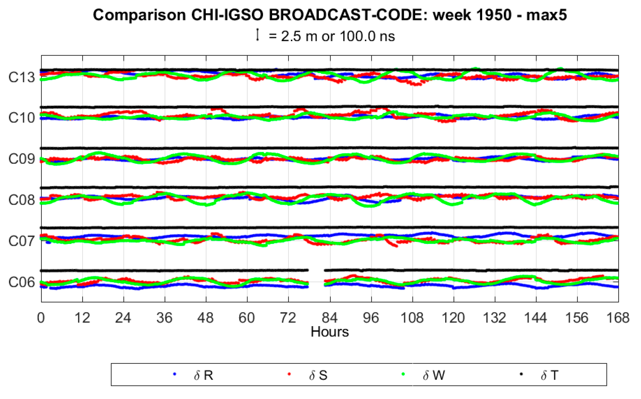

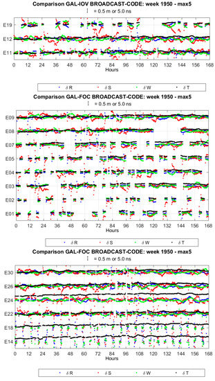
Figure A4.
Galileo coordinates and clock differences. “max 5” refers to the maximum threshold of 5 m as a condition for coordinate rejection.
Figure A4.
Galileo coordinates and clock differences. “max 5” refers to the maximum threshold of 5 m as a condition for coordinate rejection.
References
- The Multi-GNSS Experiment and Pilot Project (MGEX). Available online: http://mgex.igs.org (accessed on 29 September 2017).
- EUREF Technical Working Group (TWG). Available online: www.euref.eu/euref_twg.html (accessed on 29 September 2017).
- Montenbruck, O.; Steigenberger, P.; Hauschild, A. Broadcast versus precise ephemerides: A multi-GNSS perspective. GPS Solut. 2015, 19, 321–333. [Google Scholar] [CrossRef]
- Dalla Torre, A.; Caporali, A. An analysis of intersystem biases for multi-GNSS positioning. GPS Solut. 2015, 19, 297–307. [Google Scholar] [CrossRef]
- Caporali, A.; Nicolini, L. Interoperability of the GNSS’s for Positioning and Timing. In New Advanced GNSS and 3D Spatial Techniques; Lecture Notes in Geoinformation and Cartography; Cefalo, R., Zielinski, J., Barbarella, M., Eds.; Springer: Cham, Switzerland, 2017; pp. 73–85. ISBN 978-3-319-56218-6. [Google Scholar]
- Prange, L.; Orliac, E.; Dach, R.; Arnold, D.; Beutler, G.; Schaer, S.; Jäggi, A. CODE’s five-system orbit and clock solution—The challenges of multi-GNSS data analysis. J. Geod. 2017, 91, 345–360. [Google Scholar] [CrossRef]
- Revnivykh, S. GLONASS ground control segment: Orbit, clock, time scale and geodesy definition. In Proceedings of the 25th International Technical Meeting of the Satellite Division of the Institute of Navigation (ION GNSS 2012), Nashville, TN, USA, 17–21 September 2012; pp. 3931–3949. [Google Scholar]
- Kosenko, V. Global Navigation Satellite System (GLONASS): Status and Development. In United Nations/Russian Federation Workshop on the Applications of Global Navigation Satellite Systems; Russian Federation: Krasnoyarsk, Russia, 2015. [Google Scholar]
- Teunissen, P.J.G.; Montenbruck, O. Springer Handbook of Global Navigation Satellite Systems, 1st ed.; Springer International Publishing: Cham, Switzerland, 2017; ISBN 978-3-319-42926-7. [Google Scholar]
- Dach, R.; Lutz, S.; Walser, P.; Fridez, P. Bernese GNSS Software Version 5.2. User Manual; University of Bern, Bern Open Publishing: Bern, Switzerland, 2015; ISBN 978-3-906813-05-9. [Google Scholar]
- EU. European GNSS (Galileo) Open Service Signal in Space Interface Control Document. Available online: https://www.gsc-europa.eu/system/files/galileo_documents/Galileo-OS-SIS-ICD.pdf (accessed on 4 January 2018).
- Steigenberger, P.; Montenbruck, O. Galileo status: Orbits, clocks, and positioning. GPS Solut. 2017, 21, 319–331. [Google Scholar] [CrossRef]
- International GNSS Service (IGS) RINEX Working Group and Radio Technical Commission for Maritime Services Special Committee 104 (RTCM-SC104). RINEX The Receiver Independent Exchange Format; Version 3.03; Werner Gurtner, Astronomical Institute of the University of Bern, Switzerland and Lou Estey, UNAVCO: Boulder, CO, USA, 2015. [Google Scholar]
- Nischan, T. GFZRNX–RINEX GNSS Data Conversion and Manipulation Toolbox (Version 1.05). Available online: http://dataservices.gfz-potsdam.de/panmetaworks/showshort.php?id=escidoc:1577894 (accessed on 4 January 2018).
- Russian Institute of Space Device Engineering (RISDE). Global Navigation Satellite System GLONASS—Interface Control Document; Version 5.1; Russian Institute of Space Device Engineering: Moscow, Russia, 2008. [Google Scholar]
- Håkansson, M.; Jensen, A.B.O.; Horemuz, M.; Hedling, G. Review of code and phase biases in multi-GNSS positioning. GPS Solut. 2017, 21, 849–860. [Google Scholar] [CrossRef]
- Zeng, A.; Yang, Y.; Ming, F.; Jing, Y. BDS-GPS inter-system bias of code observation and its preliminary analysis. GPS Solut. 2017, 21, 1417–1425. [Google Scholar] [CrossRef]
- Jiang, N.; Xu, Y.; Xu, T.; Xu, G.; Sun, Z.; Schuh, H. GPS/BDS short-term ISB modelling and prediction. GPS Solut. 2017, 21, 163–175. [Google Scholar] [CrossRef]
- Odijk, D.; Teunissen, P.J.G. Characterization of between-receiver GPS-Galileo inter-system biases and their effect on mixed ambiguity resolution. GPS Solut. 2013, 17, 521–533. [Google Scholar] [CrossRef]
- Gioia, C.; Borio, D. A statistical characterization of the Galileo-to-GPS inter-system bias. J. Geod. 2016, 90, 1279–1291. [Google Scholar] [CrossRef]
- Chen, J.; Xiao, P.; Zhang, Y.; Wu, B. GPS/GLONASS System Bias Estimation and Application in GPS/GLONASS Combined Positioning. In China Satellite Navigation Conference (CSNC) 2013 Proceedings. Lecture Notes in Electrical Engineering; Sun, J., Jiao, W., Wu, H., Shi, C., Eds.; Springer: Berlin/Heidelberg, Germany, 2013; pp. 323–333. ISBN 978-3-642-37403-6. [Google Scholar]


© 2018 by the authors. Licensee MDPI, Basel, Switzerland. This article is an open access article distributed under the terms and conditions of the Creative Commons Attribution (CC BY) license (http://creativecommons.org/licenses/by/4.0/).