Estimation of Water Stress in Grapevines Using Proximal and Remote Sensing Methods †

 ,
, 

 , , , ,
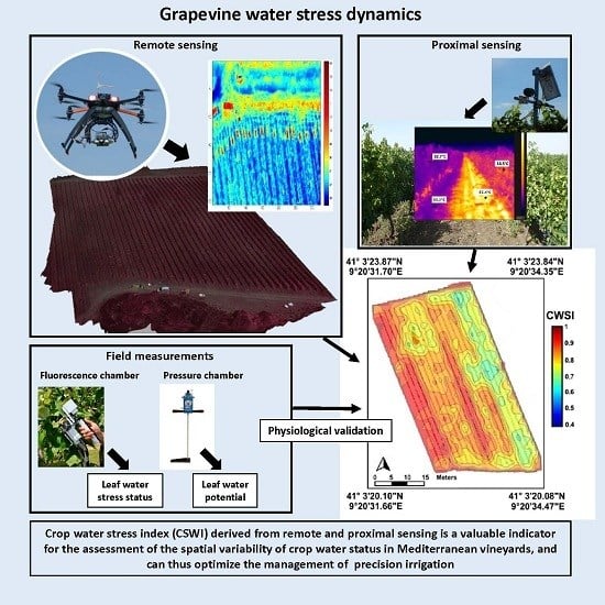
Abstract
1. Introduction
2. Materials and Methods
2.1. Experimental Sites
2.2. Remote Sensing Measurements
2.2.1. UAV Platform and Payload
2.2.2. Flight Survey
2.2.3. Remotely-Sensed Data Collection and Processing
2.3. Proximal Sensing Measurements
Infrared Thermography and Thermal Indices
2.4. Physiological Measurements
2.4.1. Stem Water Potential
2.4.2. Leaf Gas Exchange and Fluorescence
3. Results
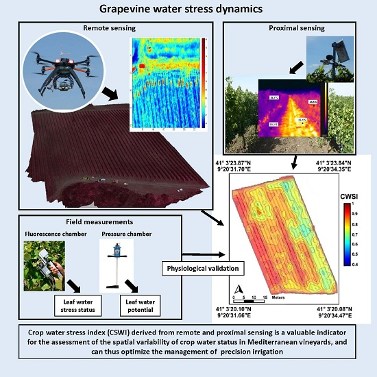
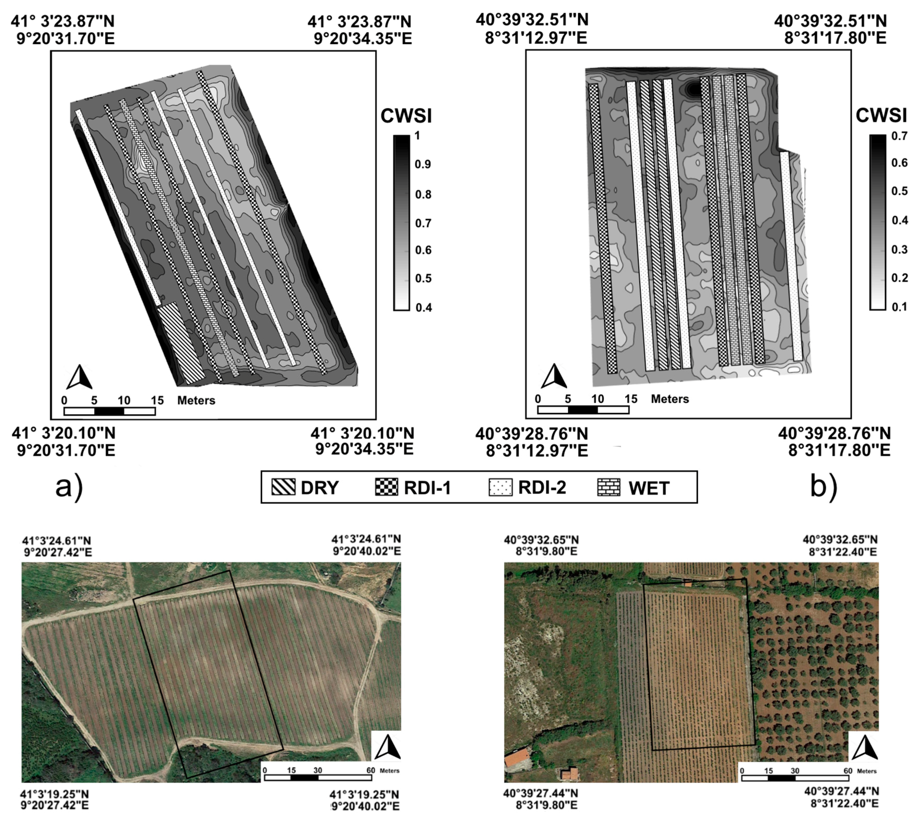
3.1. Remote Sensing Dataset
3.2. Proximal Sensing Dataset
3.3. Physiological Dataset
4. Discussion
5. Conclusions
Acknowledgments
Author Contributions
Conflicts of Interest
References
- Ojeda, H.; Andary, C.; Kraeva, E.; Carbonneau, A.; Deloire, A. Influence of pre- and post-veraison water deficit on synthesis and concentration of skin phenolic compounds during berry growth of Vitis vinifera cv Shiraz. Am. J. Enol. Viticult. 2002, 53, 261–267. [Google Scholar]
- Jackson, R.D.; Idso, S.B.; Reginato, R.J.; Pinter, P.J. Canopy temperature as a crop water stress indicator. Water Resour. Res. 1981, 17, 1133–1138. [Google Scholar] [CrossRef]
- Jones, H.G. Irrigation scheduling: Advantages and pitfalls of plant-based methods. J. Exp. Bot. 2004, 55, 2427–2436. [Google Scholar] [CrossRef] [PubMed]
- Berni, J.A.J.; Zarco-Tejada, P.J.; Sepulcre-Canto, G.; Fereres, E.; Villalobos, F. Mapping canopy conductance and CWSI in olive orchards using high resolution thermal remote sensing imagery. Remote Sens. Environ. 2009, 113, 2380–2388. [Google Scholar] [CrossRef]
- Berni, J.A.J.; Zarco-Tejada, P.J.; Suarez, L.; Fereres, E. Thermal and narrowband multispectral remote sensing for vegetation monitoring from an unmanned aerial vehicle. IEEE Trans. Geosci. Remote Sens. 2009, 47, 722–738. [Google Scholar] [CrossRef]
- Gonzalez-Dugo, V.; Zarco-Tejada, P.; Berni, J.A.J.; Suarez, L.; Goldhamer, D.; Fereres, E. Almond tree canopy temperature reveals intra-crown variability that is water stress-dependent. Agric. For. Meteorol. 2012, 154–155, 156–165. [Google Scholar] [CrossRef]
- Zarco-Tejada, P.J.; Gonzalez-Dugo, V.; Berni, J.A.J. Fluorescence, temperature and narrow-band indices acquired from a UAV platform for water stress detection using a micro-hyperspectral imager and a thermal camera. Remote Sens. Environ. 2012, 117, 322–337. [Google Scholar] [CrossRef]
- Grant, O.M.; Tronina, L.; Jones, H.G.; Chaves, M.M. Exploring thermal imaging variables for the detection of stress responses in grapevine under different irrigation regimes. J. Exp. Bot. 2007, 58, 815–825. [Google Scholar] [CrossRef] [PubMed]
- Möller, M.; Alchanatis, V.; Cohen, Y.; Meron, M.; Tsipris, J.; Naor, A.; Ostrovsky, V.; Sprintsin, M.; Cohen, S. Use of thermal and visible imagery for estimating crop water status of irrigated grapevine. J. Exp. Bot. 2007, 58, 827–838. [Google Scholar] [CrossRef] [PubMed]
- Gontia, N.K.; Tiwari, K.N. Development of crop water stress index of wheat crop for scheduling irrigation using infrared thermometry. Agric. Water Manag. 2008, 95, 1144–1152. [Google Scholar] [CrossRef]
- Jones, H.G.; Serraj, R.; Loveys, B.R.; Xiong, L.; Wheaton, A.; Price, A.H. Thermal infrared imaging of crop canopies for the remote diagnosis and quantification of plant responses to water stress in the field. Funct. Plant Biol. 2009, 36, 978–979. [Google Scholar] [CrossRef]
- Romano, G.; Zia, S.; Spreer, W.; Sanchez, C.; Cairns, J.; Araus, J.L.; Müller, J. Use of thermography for high throughput phenotyping of tropical maize adaptation in water stress. Comput. Electron. Agric. 2011, 79, 67–74. [Google Scholar] [CrossRef]
- Alchanatis, V.; Cohen, Y.; Cohen, S.; Moller, M.; Sprinstin, M.; Meron, M.; Tsipris, J.; Saranga, Y.; Sela, E. Evaluation of different approaches for estimating and mapping crop water status in cotton with thermal imaging. Precis. Agric. 2010, 11, 27–41. [Google Scholar] [CrossRef]
- Baluja, J.; Diago, M.P.; Balda, P.; Zorer, R.; Meggio, F.; Morales, F.; Tardaguila, J. Assessment of vineyard water status variability by thermal and multispectral imagery using an unmanned aerial vehicle (UAV). Irrig. Sci. 2012, 30, 511–522. [Google Scholar] [CrossRef]
- Bellvert, J.; Zarco-Tejada, P.J.; Girona, J.; Fereres, E. Mapping crop water stress index in a ‘Pinot-noir’ vineyard: Comparing ground measurements with thermal remote sensing imagery from an unmanned aerial vehicle. Precis. Agric. 2014, 15, 361–376. [Google Scholar] [CrossRef]
- Gonzalez-Dugo, V.; Zarco-Tejada, P.; Nicolas, E.; Nortes, P.A.; Alarcon, J.J.; Intrigliolo, D.S.; Fereres, E. Using high resolution UAV thermal imagery to assess the variability in the water status of five fruit tree species within a commercial orchard. Precis. Agric. 2013, 14, 660–678. [Google Scholar] [CrossRef]
- Humplík, J.F.; Lazár, D.; Husičková, A.; Spíchal, L. Automated phenotyping of plant shoots using imaging methods for analysis of plant stress responses—A review. Plant Methods 2015, 11, 29. [Google Scholar] [CrossRef] [PubMed]
- Nilsson, H.E. Remote sensing and image analysis in plant pathology. Annu. Rev. Phytopathol. 1995, 15, 489–527. [Google Scholar] [CrossRef] [PubMed]
- Peñuelas, J.; Filella, I. Visible and near-infrared reflectance techniques for diagnosing plant physiological status. Trends Plant Sci. 1998, 3, 151–156. [Google Scholar] [CrossRef]
- Lichtenthaler, H.K.; Miehé, J.A. Fluorescence imaging as a diagnostic tool for plant stress. Trends Plant Sci. 1997, 2, 316–320. [Google Scholar] [CrossRef]
- Riccardi, M.; Mele, G.; Pulvento, C.; Lavini, A.; d’Andria, R.; Jacobsen, S.E. Non-destructive evaluation of chlorophyll content in quinoa and amaranth leaves by simple and multiple regression analysis of RGB image components. Photosynth. Res. 2014, 120, 263–272. [Google Scholar] [CrossRef] [PubMed]
- Salazar-Parra, C.; Aguirreolea, J.; Sànchez-Dìaz, M.; Irigoyen, J.J.; Morales, F. Photosynthetic response of Tempranillo grapevine to climate change scenarios. Ann. Appl. Biol. 2012, 161, 277–292. [Google Scholar] [CrossRef]
- Demmig-Adams, B.; Adams, W.W., III; Barker, D.H.; Logan, B.A.; Bowling, D.R.; Verhoeven, A.S. Using chlorophyll fluorescence to assess the fraction of absorbed light allocated to thermal dissipation of excess excitation. Physiol. Plant. 1996, 98, 253–264. [Google Scholar] [CrossRef]
- Baker, N.R.; Rosenqvist, E. Applications of chlorophyll fluorescence can improve crop production strategies: An examination of future possibilities. J. Exp. Bot. 2004, 55, 1607–1621. [Google Scholar] [CrossRef] [PubMed]
- Borawska-Jarmułowicz, B.; Mastalerczuk, G.; Pietkiewicz, S.; Kalaji, M.H. Low temperature and hardening effects on photosynthetic apparatus efficiency and survival of forage grass varieties. Plant Soil Environ. 2014, 60, 177–183. [Google Scholar]
- Maxwell, K.; Johnson, G.N. Chlorophyll fluorescence—A practical guide. J. Exp. Bot. 2000, 51, 659–668. [Google Scholar] [CrossRef] [PubMed]
- Kalaji, H.M.; Schansker, G.; Ladle, R.J.; Goltsev, V.; Bosa, K.; Allakhverdiev, S.I.; Brestic, M.; Bussotti, F.; Calatayud, A.; Dąbrowski, P.; et al. Frequently asked questions about in vivo chlorophyll fluorescence: Practical issues. Photosynth. Res. 2014, 121, 122–158. [Google Scholar] [CrossRef] [PubMed]
- Jones, H.G.; Vaughan, R.A. Remote Sensing of Vegetation: Principles, Techniques, and Applications; Oxford University Press: Oxford, UK, 2010; ISBN 9780199207794. [Google Scholar]
- Idso, S.B.; Jackson, R.D.; Pinter, P.J.; Reginato, R.J.; Hatfield, J.L. Normalizing the stress degree day parameter for environmental variability. Agric. Meteorol. 1981, 24, 45–55. [Google Scholar] [CrossRef]
- Jones, H.G.; Stoll, M.; Santos, T.; de Sousa, C.; Chaves, M.M.; Grant, O.M. Use of infrared thermography for monitoring stomatal closure in the field: Application to grapevine. J. Exp. Bot. 2002, 53, 2249–2260. [Google Scholar] [CrossRef] [PubMed]
- Matese, A.; Di Gennaro, S.F.; Berton, A. Assessment of a canopy height model (CHM) in a vineyard using UAV-based multispectral imaging. Int. J. Remote Sens. 2017, 38, 2150–2160. [Google Scholar] [CrossRef]
- Leinonen, I.; Jones, H.G. Combining thermal and visible imagery for estimating canopy temperature and identifying plant stress. J. Exp. Bot. 2004, 55, 1423–1431. [Google Scholar] [CrossRef] [PubMed]
- Costa, J.M.; Ortuño, M.F.; Lopes, C.M.; Chaves, M.M. Grapevine varieties exhibiting differences in stomatal response to water deficit. Funct. Plant Biol. 2012, 39, 179–189. [Google Scholar] [CrossRef]
- Pou, A.; Diago, M.P.; Medrano, H.; Baluja, J.; Tardaguila, J. Validation of thermal indices for water stress status identification in grapevine. Agric. Water Manag. 2014, 134, 60–72. [Google Scholar] [CrossRef]
- Loveys, B.R.; Jones, H.G.; Theobald, J.C.; McCarthy, M.G. An assessment of plant-based measures of grapevine performance as irrigation-scheduling tools. Acta Hortic. 2008, 792, 391–403. [Google Scholar] [CrossRef]
- Van Kooten, O.; Snel, J.F. The use of chlorophyll fluorescence nomenclature in plant stress physiology. Photosynth. Res. 1990, 25, 147–150. [Google Scholar] [CrossRef] [PubMed]
- Giorio, P. Black leaf-clips increased minimum fluorescence emission in clipped leaves exposed to high solar radiation during dark adaptation. Photosynthetica 2011, 49, 371–379. [Google Scholar] [CrossRef]
- Tisseyre, B.; Ducanchez, A. Spatial variability of drip irrigation in small vine fields of south of France. In Precision Agriculture ‘13; Stafford, J.V., Ed.; Wageningen Academic Publishers: Wageningen, The Netherlands, 2013; pp. 251–257. [Google Scholar]
- García-Tejero, I.F.; Costa, J.M.; Egipto, R.; Durán-Zuazo, V.H.; Lima, R.S.N.; Lopes, C.M.; Chaves, M.M. Thermal data to monitor crop-water status in irrigated Mediterranean viticulture. Agric. Water Manag. 2016, 176, 80–90. [Google Scholar] [CrossRef]
- Wang, Z.Z.; Zheng, P.; Meng, J.F.; Xi, Z.M. Effect of exogenous 24-epibrassinolide on chlorophyll fluorescence, leaf surface morphology and cellular ultrastructure of grape seedlings (Vitis vinifera L.) under water stress. Acta Physiol. Plant. 2015, 37, 1729–1740. [Google Scholar] [CrossRef]
- Flexas, J.; Bota, J.; Escalona, J.M.; Sampol, B.; Medrano, H. Effects of drought on photosynthesis in grapevines under field conditions: An evaluation of stomatal and mesophyll limitations. Funct. Plant Biol. 2002, 29, 461–471. [Google Scholar] [CrossRef]
- Flexas, J.; Escalona, J.M.; Medrano, H. Down-regulation of photosynthesis by drought under field conditions in grapevine leaves. Aust. J. Plant Physiol. 1998, 25, 892–900. [Google Scholar] [CrossRef]
- Flexas, J.; Ribas-Carbò, M.; Dìaz-Espejo, A.; Galmès, J.; Medrano, H. Mesophyll conductance to CO2: Current knowledge and future prospects. Plant Cell Environ. 2008, 31, 602–621. [Google Scholar] [CrossRef] [PubMed]
- Björkman, O.; Demmig, B. Photon yield of O2 evolution and chlorophyll fluorescence characteristics of 77K among vascular plants of diverse origins. Planta 1987, 170, 489–504. [Google Scholar] [CrossRef] [PubMed]
- Morales, F.; Abadía, A.; Abadía, J. Chlorophyll fluorescence and photon yield of oxygen evolution in iron-deficient sugar beet (Beta vulgaris L.) leaves. Plant Physiol. 1991, 97, 866–893. [Google Scholar] [CrossRef]
- Ripullone, F.; Rivelli, A.R.; Baraldi, R.; Guarini, R.; Guerrieri, R.; Magnani, F.; Peñuelas, J.; Raddi, S.; Borghetti, M. Effectiveness of the photochemical reflectance index to track photosynthetic activity over a range of forest tree species and plant water status. Funct. Plant Biol. 2011, 38, 177–186. [Google Scholar] [CrossRef]
- Morales, F.; Abadìa, A.; Abadìa, J. Photoinhibition and photoprotection under nutrient deficiencies, drought and salinity. In Photoprotection, Photoinhibition, Gene Regulation and Environment; Demming-Adams, B., Adams, W.W., III, Mattoo, A.K., Eds.; Springer: Dordrecht, The Netherlands, 2006; pp. 65–85. [Google Scholar]
- Grant, O.M.; Tronina, L.; Ramalho, J.C.; Besson, C.K.; Lobo-Do-Vale, R.; Pereira, J.S.; Jones, H.G.; Chaves, M.M. The impact of drought on leaf physiology of Quercus suber L. trees: Comparison of an extreme drought event with chronic rainfall reduction. J. Exp. Bot. 2010, 61, 4361–4371. [Google Scholar] [CrossRef] [PubMed]
- Pascual, I.; Azcona, I.; Morales, F.; Aguirreole, J.; Sànchez-Dìaz, M. Photosynthetic response of pepper plants to wilt induced by Verticillium dahliae and soil water deficit. J. Plant Physiol. 2010, 167, 701–708. [Google Scholar] [CrossRef] [PubMed]
- Hu, W.H.; Yan, X.H.; Xiao, Y.A.; Zeng, J.J.; Qi, H.J.; Ogweno, J.O. 24-Epibrassinosteroid alleviate drought-induced inhibition of photosynthesis in Capsicum annuum. Sci. Hortic. 2013, 150, 232–237. [Google Scholar] [CrossRef]
- Qin, H.Y.; Ai, J.; Xu, P.L.; Wang, Z.X.; Zhao, Y.; Yang, Y.M.; Fan, S.T.; Shen, Y.J. Chlorophyll fluorescence parameters and ultrastructure in amur grape (Vitis amurensis Rupr.) under salt stress. Acta Bot. Boreal. Occident. Sin. 2013, 33, 1159–1164. [Google Scholar]
- Jones, H.G. Use of infrared thermometry for estimation of stomatal conductance in irrigation scheduling. Agric. For. Meteorol. 1999, 95, 139–149. [Google Scholar] [CrossRef]
- Santesteban, L.; Di Gennaro, S.; Herrero-Langreo, A.; Miranda, C.; Royo, J.; Matese, A. High-resolution uav-based thermal imaging to estimate the instantaneous and seasonal variability of plant water status within a vineyard. Agric. Water Manag. 2017, 183, 49–59. [Google Scholar] [CrossRef]
- Hoffmann, H.; Jensen, R.; Thomsen, A.; Nieto, H.; Rasmussen, J.; Friborg, T. Crop water stress maps for an entire growing season from visible and thermal UAV imagery. Biogeosciences 2016, 13, 6545–6563. [Google Scholar] [CrossRef]
- Espinoza, C.Z.; Khot, L.R.; Sankaran, S.; Jacoby, P.W. High Resolution Multispectral and Thermal Remote Sensing-Based Water Stress Assessment in Subsurface Irrigated Grapevines. Remote Sens. 2017, 9, 961. [Google Scholar] [CrossRef]


| Vineyard | Treatment | May (MPa) | June (MPa) | July (MPa) | August (MPa) | September (MPa) | Irrigation Number (n) | Irrigation Volume (m3 ha−1) |
|---|---|---|---|---|---|---|---|---|
| Arzachena | RDI-1 | −0.6 | −0.9 | −0.9 | −0.9 | −1.4 | 9 | 768 |
| RDI-2 | −0.6 | −1.2 | −1.2 | −1.2 | −1.4 | 6 | 472 | |
| Usini | RDI-1 | −0.6 | −0.9 | −0.9 | −0.9 | −1.4 | 2 | 366 |
| RDI-2 | −0.6 | −1.2 | −1.2 | −1.2 | −1.4 | 1 | 133 |
| Arzachena | Usini | |
|---|---|---|
| Twet (remote procedure) | 23 | 25 |
| Tdry (remote procedure) | 46 | 43 |
| Twet (ground procedure) | 32 | 27 |
| Tdry (ground procedure) | 41 | 35 |
| White panel | 35 | 32 |
| Blue panel | 56 | 53 |
| Black panel | 68 | 67 |
| ‘Vermentino’ | ‘Cabernet’ | ‘Cagnulari’ | |
|---|---|---|---|
| CWSI | |||
| Wet | 0.77 ± 0.08 a | 0.22 ± 0.03 a | 0.34 ± 0.04 a |
| RDI-1 | 0.72 ± 0.09 a | 0.28 ± 0.04 b | 0.43 ± 0.05 ab |
| RDI-2 | 0.90 ± 0.06 b | 0.34 ± 0.05 c | 0.51 ± 0.12 b |
| Dry | 0.97 ± 0.03 b | 0.47 ± 0.02 d | 0.63 ± 0.04 c |
| ‘Vermentino’ | ‘Cabernet’ | ‘Cagnulari’ | |
|---|---|---|---|
| Stem Water Potential (MPa) | |||
| Wet | −0.78 ± 0.03 b | −0.43 ± 0.01 d | −0.54 ± 0.02 b |
| RDI-1 | −0.96 ± 0.05 b | −0.82 ± 0.09 c | −0.71 ± 0.10 b |
| RDI-2 | −1.27 ± 0.03 a | −1.06 ± 0.64 b | −1.13 ± 0.05 a |
| Dry | −1.34 ± 0.09 a | −1.31 ± 0.03 a | −1.26 ± 0.01 a |
| ’Vermentino’ | ||||||
| Pn | Gs | Fv/Fm | Fv’/Fm’ | ΦPSII | NPQ | |
| µmol m−2 s−1 | mmol m−2 s−1 | |||||
| Wet | 6.5 ± 0.3 a | 0.27 ± 0.04 a | 0.8 ± 0.01 a | 0.4 ± 0.01 a | 0.2 ± 0.03 a | 2.1 ± 0.2 b |
| RDI-1 | 6.3 ± 0.7 a | 0.26 ± 0.04 a | 0.8 ± 0.01 a | 0.4 ± 0.01 a | 0.2 ± 0.02 a | 2.2 ± 0.2 b |
| RDI-2 | 2.5 ± 0.5 b | 0.07 ± 0.02 b | 0.8 ± 0.01 a | 0.3 ± 0.02 b | 0.1 ± 0.01 b | 3.1 ± 0.2 a |
| Dry | 2.6 ± 0.7 b | 0.06 ± 0.01 b | 0.8 ± 0.01 a | 0.4 ± 0.02 b | 0.1 ± 0.01 b | 2.8 ± 0.2 a |
| ‘Cabernet’ | ||||||
| Pn | Gs | Fv/Fm | Fv’/Fm’ | ΦPSII | NPQ | |
| µmol m−2 s−1 | mmol m−2 s−1 | |||||
| Wet | 15.9 ± 1.1 a | 0.39 ± 0.09 a | 0.8 ± 0.01 a | 0.3 ± 0.01 a | 0.1 ± 0.01 a | 2.2 ± 0.01a |
| RDI-1 | 13.0 ± 0.9 ab | 0.32 ± 0.07 ab | 0.8 ± 0.01 a | 0.4 ± 0.02 a | 0.1 ± 0.03 ab | 2.3 ± 0.02 ab |
| RDI-2 | 10.1 ± 2.6 b | 0.17 ± 0.05 ab | 0.8 ± 0.01 a | 0.4 ± 0.02 a | 0.1 ± 0.03 ab | 2.0 ± 0.02 ab |
| Dry | 5.8 ± 1.5 b | 0.12 ± 0.03 b | 0.8 ± 0.01 a | 0.3 ± 0.02 b | 0.1 ± 0.01 b | 2.6 ± 0.02 b |
| ‘Cagnulari’ | ||||||
| Pn | Gs | Fv/Fm | Fv’/Fm’ | ΦPSII | NPQ | |
| µmol m−2 s−1 | mmol m−2 s−1 | |||||
| Wet | 14.7 ± 1.3 a | 0.35 ± 0.05 a | 0.8 ± 0.01 a | 0.4 ± 0.02 a | 0.1 ± 0.02 a | 1.8 ± 0.2 b |
| RDI-1 | 12.1 ± 0.9 ab | 0.28 ± 0.04 ab | 0.8 ± 0.01 a | 0.4 ± 0.04 a | 0.1 ± 0.03 a | 2.0 ± 0.3 a |
| RDI-2 | 9.2 ± 1.1 b | 0.17 ± 0.05 bc | 0.8 ± 0.01 a | 0.4 ± 0.03 a | 0.1 ± 0.01 a | 2.0 ± 0.2 a |
| Dry | 5.3 ± 0.2 b | 0.12 ± 0.03 c | 0.8 ± 0.01 a | 0.4 ± 0.02 b | 0.1 ± 0.02 b | 2.5 ± 0.3 a |
| Cultivars | CTleaf | Fv’/Fm’ | NPQ | ΦPSII | Pn |
|---|---|---|---|---|---|
| ‘Vermentino’ | 0.49 *** | −0.43 ** | 0.47 ** | −0.35 * | −0.55 *** |
| ‘Cabernet’ | 0.75 **** | −0.37 * | 0.27 ns | −0.16 ns | −0.66 *** |
| ‘Cagnulari’ | 0.63 *** | −0.48 * | 0.09 ns | −0.49 * | −0.80 **** |
© 2018 by the authors. Licensee MDPI, Basel, Switzerland. This article is an open access article distributed under the terms and conditions of the Creative Commons Attribution (CC BY) license (http://creativecommons.org/licenses/by/4.0/).
Share and Cite
Matese, A.; Baraldi, R.; Berton, A.; Cesaraccio, C.; Di Gennaro, S.F.; Duce, P.; Facini, O.; Mameli, M.G.; Piga, A.; Zaldei, A. Estimation of Water Stress in Grapevines Using Proximal and Remote Sensing Methods. Remote Sens. 2018, 10, 114. https://doi.org/10.3390/rs10010114
Matese A, Baraldi R, Berton A, Cesaraccio C, Di Gennaro SF, Duce P, Facini O, Mameli MG, Piga A, Zaldei A. Estimation of Water Stress in Grapevines Using Proximal and Remote Sensing Methods. Remote Sensing. 2018; 10(1):114. https://doi.org/10.3390/rs10010114
Chicago/Turabian StyleMatese, Alessandro, Rita Baraldi, Andrea Berton, Carla Cesaraccio, Salvatore Filippo Di Gennaro, Pierpaolo Duce, Osvaldo Facini, Massimiliano Giuseppe Mameli, Alessandra Piga, and Alessandro Zaldei. 2018. "Estimation of Water Stress in Grapevines Using Proximal and Remote Sensing Methods" Remote Sensing 10, no. 1: 114. https://doi.org/10.3390/rs10010114
APA StyleMatese, A., Baraldi, R., Berton, A., Cesaraccio, C., Di Gennaro, S. F., Duce, P., Facini, O., Mameli, M. G., Piga, A., & Zaldei, A. (2018). Estimation of Water Stress in Grapevines Using Proximal and Remote Sensing Methods. Remote Sensing, 10(1), 114. https://doi.org/10.3390/rs10010114