4.1. System Design
The new system made it possible to conduct age categorization of stocks (separation of product into different stocks and thus determination of different shelf life). This allows the products with different shelf lives to have different prices. This, in return, will make it possible for customers to make comparisons among products. Wastage costs of the products whose self-lives are about to expire and not sold sometimes reach serious levels. However, when spoilage losses increase, organizations firstly question appropriateness of the size of the order placed for the concerned product.
However, most of the time, the first mistake is to decide on size of the group ordered based on follow-ups of the stock cycle speed again. Actually, what needs to be done in such a case is to implement new pricing strategies and different sale techniques, instead of revising the size of the groups ordered through controls of the stock cycle speed. This would allow organizations to increase their revenue and profit rates, as well as enhance the efficiency of the sale and stock cycle of products. Staleness degree of products has exponential distribution. In other words, the lengths of time within which products remain on shelves decrease their preferability for customers. For this reason, the preferability of products decreases in parallel to declining freshness status.
The dynamic promotions in the prices of products directly affect customers’ attitudes towards purchase. This approach increases revenue earned, but it brings limited improvement on profit of organizations. This is because sale rate increase continuously occurs on products with high freshness status to a certain extent. However, the real issue, in the opinion of the organization, is the need to increase revenue by increasing the sales of products about to become stale, and accordingly to decrease spoilage costs through these sales and increase the profit.
4.2. Scenario Definition
Under the present study, dynamism of pricing system modeled with GAMS software program varies according to the staleness degree of product stocks. The present study explored two different scenarios in line with differences among stocks in terms of age profiles (freshness status) and different dynamic pricing strategies. These scenarios sought to maximize profit by using different pricing formula.
In the first scenario, pricing is made dynamic with the assumption that pricing of each stock of a product is affected only by its own staleness degree.
The second scenario assumed that staleness degree of different stocks of a product on shelves simultaneously has multiplying effect (all stocks on shelves are affected by the staleness rate and their prices are determined accordingly).
In the third scenario, the freshness rate of different products stocks, which are determined in the same discount group by the supermarket managers, affect each stock’s price dynamically. The decision of the related products is very important for low pricing type. The last scenario is inspired from Turkey’s real applications in the supermarkets. In the last day of the perishable products, markets want to sell total amount of the stocks to the wholesale buyer instead of selling to the customer one by one. These types of customers (wholesalers) are usually patisseries and bakery markets. Alternatively, sometimes the supermarkets use their own nearly perished products to cook some fresh foods in their patisserie department. To sell all in the last day instead of being wasted, the markets price this type of products at very low (deep) price. The results obtained through these scenarios are compared with the real size of the order (stock amount), sale prices and sale amounts of a real and big supermarket with high profit margin in Turkey. The system comparisons based on the findings obtained are presented in the following tables and figures.
The present study analyses the impact of dynamic pricing on total sale amount, total profit and spoilage amount. It is assumed that the system operates continuously and it can be renewed under deterministic demand within a determined period of time (orders are placed continuously) and the demand has price elasticity. The degree of response shown by consumers (sensitivity degree) to changes in price in the form of changing the amount of product they buy is defined as price elasticity of demand. In the present study, elasticity of price is provided with a coefficient.
At the stage of modeling, perishable products, their stocks and the number of days they have remained on shelves are stated separately. It is assumed that the product does not have starting stock and that the number of product stocks is controlled separately every day. The intervals between the orders are not fixed. In addition, it is assumed that the duration within which orders are delivered to supermarkets and the sizes of orders are variable.
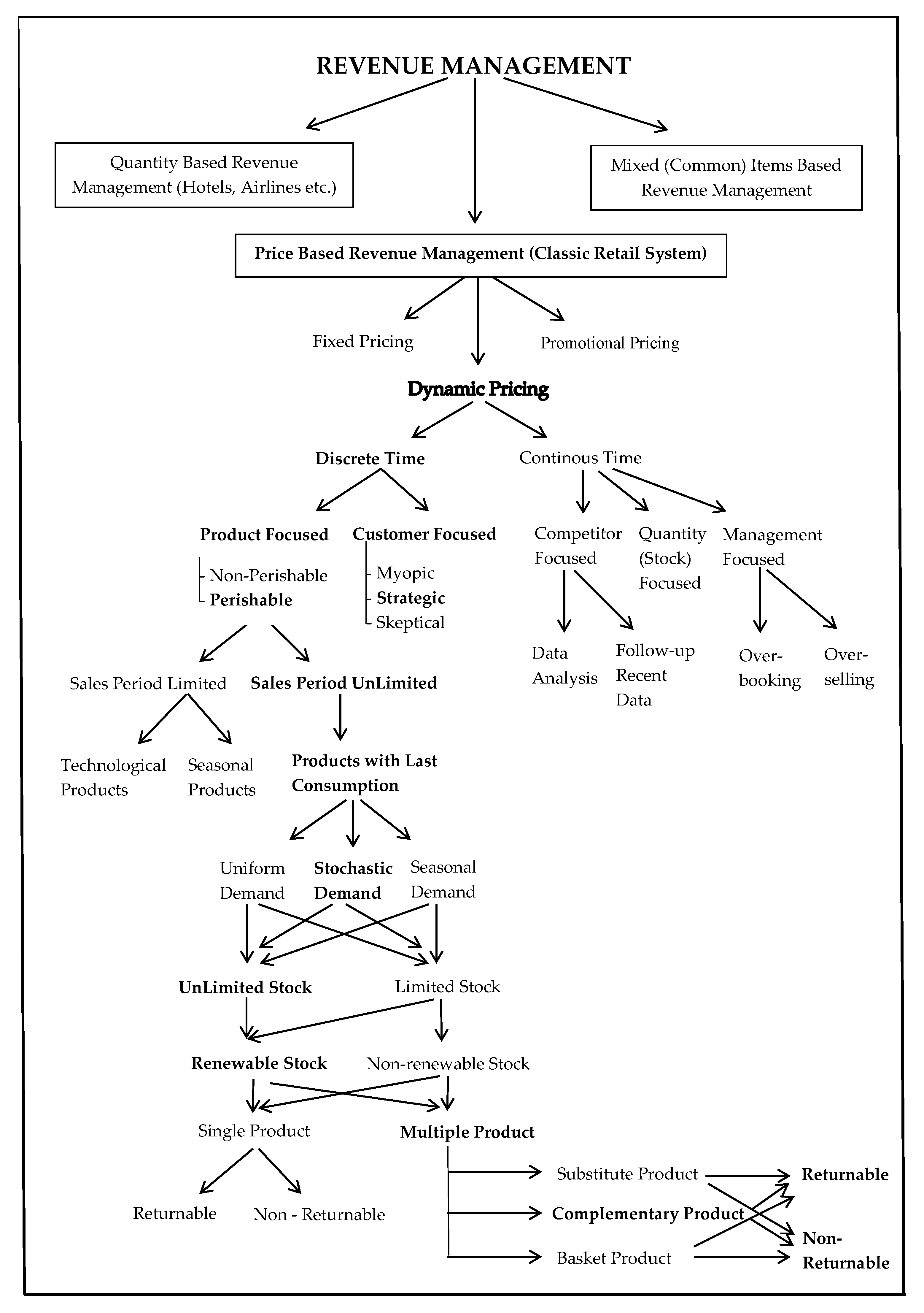
The products with 0 shelf-life and the unsold ones are defined as stale products and they are removed from shelves. For this reason, different stocks of products are sometimes displayed on shelves simultaneously, and same group stocks of a product with the same shelf life are sometimes displayed on shelves together, as well. The work flow of different scenario based models is shown in detail in
Figure 2. The system of the proposed model continues to work until the end of the market decision period. In addition, the limits of each product freshness rates, such as x and y, are determined by the supermarket’s top managers depending on the products sales rate. Thus, every product life cycle sustainability and customer attitudes change in different scenarios.
4.3. Problem Formulation
The objective of supermarkets is to maximize the expected profit. However, the revenue management system of the markets has several different significant constraints. Thus, the system is so complex and it should be strategically managed. The aim of this paper is to mitigation of spoilage rates of perishable products by applying dynamic pricing strategies. Thus, the system is conducted with a deterministic model approach in consideration of various factors, such as interaction between freshness/staleness degrees of different groups of products, elasticity of demand against price and sensitivity of demand towards freshness degree. All the indexes and notations of the proposed model are shown as below.
Indexes
| Product index |
| Stock index |
| Time period index |
Parameters and Variables
| The freshness rate of the product inventories |
| The total rafted time of the product |
| The duration of the transportation delay |
| The shelf life of the product |
| Total daily product demand |
| Total daily customer demand |
| The number of total stocks on the date of t |
| The total unsold inventory of the product on the last day of its shelf life |
| The total demand of the product stocks during their shelf lives |
| The total amount of the products entered into stocks from supplier |
| The total number of the unsold/perished products |
| The number of customer arrivals to the supermarkets on the date of t |
| Number of the unmet customer orders during product shelf life |
| The number of the daily unmet customer orders |
| The unit price of the product’s waste cost (product return cost from supermarket to the manufacturer or directly idle product cost) |
| The unit price of the product setup cost |
| The unit price of the products holding cost |
| The unit unmet price of the products |
| Total daily demand rate by customer arrivals |
| Binary variable for setup costs of the products [0, 1] |
| The purchasing price of the product stocks |
| Deep selling price in very low customer demand and freshness rate |
| Low selling price in low customer demand and freshness rate |
| Medium selling price in average customer demand and freshness rate |
| High selling price in peak customer demand and freshness rate |
| Fixed selling price of the product stocks recommended by supplier or manufacturer |
Constants
, , , , , , , , , , ,
The staleness degree of products is calculated by dividing the number of days a product remains in stock to its sell-by-date. Freshness degree can be easily calculated by deducting from 1. This constraint is the most important criteria in determination of different price values to be given to different stocks in particular. During concurrent pricing of more than one stock group, the freshness degree of each product inevitably and dynamically affects the prices of other stock groups, through multiplier effect.
The number of perishable products is very high in supermarkets as mentioned previously. For this reason, the present study applied constraints on product structure/specification. The products with more intensive wastage rate are identified, and generally sale of perishable products is more problematic for supermarkets, which negatively affects profit margin. For this reason, the study is expected to cover products with a maximum remaining shelf life. In other words, the study attempts to perform production categorization under this constraint. All the notations for new system design are shown in
Figure 2. In addition, the study covers fast-moving consumer goods. For this reason, shelf life should not be more than
q days.
The value range accommodating prices should be kept limited when the prices of products are calculated daily as they change dynamically. This limits the extent to which the minimum selling price of product can be lower or higher than its purchasing price; in line with the rates to be determined by top management of supermarket. In addition, the initial sale price of product may be determined by organization accordingly.
Customers create a certain demand after they evaluate the freshness degree of all stocks made available for the product on that day and the dynamic price charged for the product by the supermarket.
In other words, the total demand occurred for the product within the implementation period is the total demand shown for all stocks of the product within time intervals specified.
If the product groups in the stocks are bigger than the demand, the products will become stale. This is very important for supermarkets as it incurs return or wastage cost. The account of stale products is formulated as follows.
If the amounts of product groups regularly ordered by supermarkets are lower than the amount of demand, the supermarkets will not provide the products desired by customers. This indicates that the maximum revenue cannot be achieved. This is to say that the organizations will suffer loss from their revenue.
The number of customers visiting supermarkets and shopping or leaving without shopping varies from day to day. This constraint is applied in order to reveal the link between the number of daily visits paid by the customers to supermarket and the number of products sold. Thanks to this constraint, increases and decreases in sales will not be taken alone on daily basis. This constraint serves as a dynamic input for the system by measuring the attention showed by customers to pricing, in other words, the performance of customer attitudes formed in response to pricing. Calculation of sale rate based on the number of customers visiting supermarket daily, which is missing in evaluations, will make it easier to evaluate revenue more efficiently. The study will include this constraint to the evaluation during the determination of discount start time of product. The management of organizations operates the system dynamically by deciding on scenarios to be implemented on prices in line with this constraint.
The amount of stocks is one of the important factors which affect the customer attitudes to purchase and organization’s profitability (in terms of whether the orders placed are used efficiently or not). Stock status is among the determinants of sizes of order groups and frequencies at which orders are placed.
The price including the discount made by supplier in cases of high amount purchased is formulated as follows:
In the cases of high purchase amounts, the costs of keeping products in stock are variable for organizations. Pricing policies determined in accordance with the degrees of freshness, staleness and customer demand at different times are very important for profitability of companies. Different dynamic scenarios planned to be implemented at different times are defined as follows.
The first thing to be determined as the decision variable of the mathematical model is the price of products. These prices will play a determinant role in the model in line with the demands shown for the freshness status and products. When the degree of freshness of products or demand of customers for products decreases, top managements of supermarkets decide to implement various price policies (scenarios) for the purpose of boosting their sales, as seen in the
Table 1. However, the present study seeks to determine the prices easily by using the model created under the above-mentioned constraints. To this end, the dynamic product pricings with formulas that belong to the scenarios developed are calculated under the model and presented to the customers. In this regard, the prices given to products under various constraints are formulated as follows.
The new pricing approach described above is re-formalized for minimizing customer preference of the freshest products as a result of joint and concurrent pricing of various groups of products (substitutions). It is a common customer practice to choose the freshest products/groups when they all have the same price. This pricing formula is based on the assumption that product interactions and freshness of degradable products are exponentially distributed. However, when supermarkets differentiate the price of each group of products, it could decrease the amount of unsold products.
The present study seeks to increase the sale of products by differentiating the prices of product stocks with different features at the right extents and amounts. In addition, another innovative aspect of the present study, which is not present in other studies, is that different freshness degrees of different groups of products affect each other’s freshness degrees and thus decrease sales (affects the purchase attitude of customers significantly). It is very important that these products, which interact with each other in ways that cannot be ignored, are sold for dynamic prices and offered to customers at the right time, and with the right strategies.
The real objective of the present study is to sell perishable products whose shelf lives are close to the end at the very best prices and with the best product stock combinations. The other objectives of the model developed under the present study are to enhance the potential to sell products to customers and thus minimize the returns of products and spoilage costs of products, all of which, in return, will furnish supermarkets with a sale and pricing policy which can bring highest profit. Sub-functions of the objective function can be described as below. The objective function is not only to maximize the revenue, but also to minimize the cost at the same time. The unique decision variable of the system is product price in this model.
or
4.4. Numerical Simulation
In this section, a case study is carried out for clear understanding of the system. Four different scenarios are used to show the results of the dynamic selling price cases. Price discounts are defined according to the freshness of the products and customer density function. Thus, the system compares the real-time pricing methodology and scenario based cases. The proposed model data are given in
Table 2,
Table 3,
Table 4 and
Table 5. All cases are compared with each other in the following parts.
Four product samples with a shelf life of 6–15 days are selected as an example for this part. The product arrival time is taken as three days for the first and third products, four days for the second and two days for the last one. In addition, some more information is given in
Table 6. All scenarios are simulated via GAMS for different time periods. The positive improvements or negative effects on revenue, cost and profit are explained in the following parts. The operation times are tried in long term for 30 days. At the end of the assessment, the effects of different pricing scenarios on the product prices are shown in the following Tables and Figures.
All type of products has different setup, waste and holding costs. In addition, if the customer demand is not being met because of small amount of stock/order, the costs for each sample products are defined in
Table 2. The numerical simulation is made for four complementary milk products in the supermarkets. The costs and profits balance from the sale of four sample perishable products, which are generally preferred together by the customer shopping, have been determined according to the respective price policies. Amount of orders for ten different groups of products is given in
Table 3. Due to inflation and so on, the purchase price of each product stocks varies in the markets, as seen in
Table 4. Customer demand is used in the system modeling for 30 days, although customer demand rate is given for 12 days as a sample in
Table 5.
All the real life parameters and data are used in the numerical simulation part. The customers buy these products together or individually every day in 30 days. Although the total demands of each product are given in
Table 7 for a month to show the data used in real life pricing type, the customer demands on different stocks of each product are classified in
Table 6 to show the differences between this paper and reality. For instance, the demand of second product on ninth day is totally 23, as clearly seen in
Table 7.
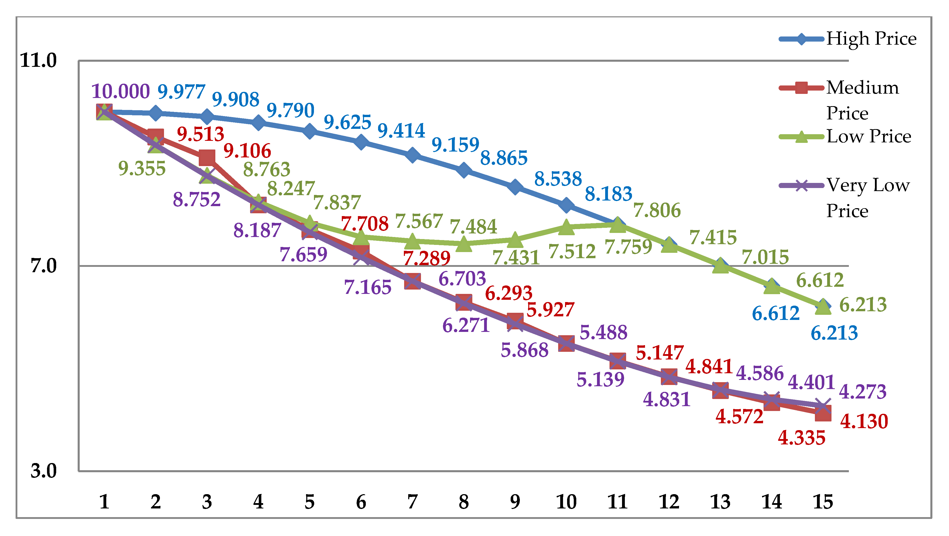
However, the products chosen by customers have three different stock types: seven demanded for first group; six demanded for second; and 10 for third group of the product. The first product is selected as an example to show that how the price is changing from the initial price to the end. It is clearly seen in
Figure 3 that high pricing strategy and low one follow a similar path after the freshness rate of 0.33 (after 11th day of its shelf-life). Thus, when the staleness rate is getting higher, the pricing strategies are working in the same way. In addition, the medium pricing strategy and very low (deep) one reach the same price at the end of life cycle of the product. All other products, 2–4, have the similar solutions as the first product. All other product prices have the same way trend, as seen in
Figure 3 and
Table 8,
Table 9 and
Table 10.
It is clearly seen from the proposed model data that high pricing is decreased slowly daily. The initial price of the products is decreased approximately 30%–35% at the end of the shelf-life in high pricing strategy. In medium pricing strategy, the price of the products is decreased suddenly after the freshness rate 0.5. When the staleness rate nearly reaches 0.75, the second sharp pricing promotion is used to accelerate the sales of the products. This pricing depends on the freshness status of the same product stocks. Thus, every different stock of the same product on the shelves effects the pricing of others to differentiate the product stocks.
The other case, as compared with this first two strategies, is low pricing. This promotion type has a group of complementary products in the milk product department. The top managers in the supermarkets decide which type of products is sold together more effectively. The freshness rate of all stocks of each product in the same promotion group affects the others dynamically.
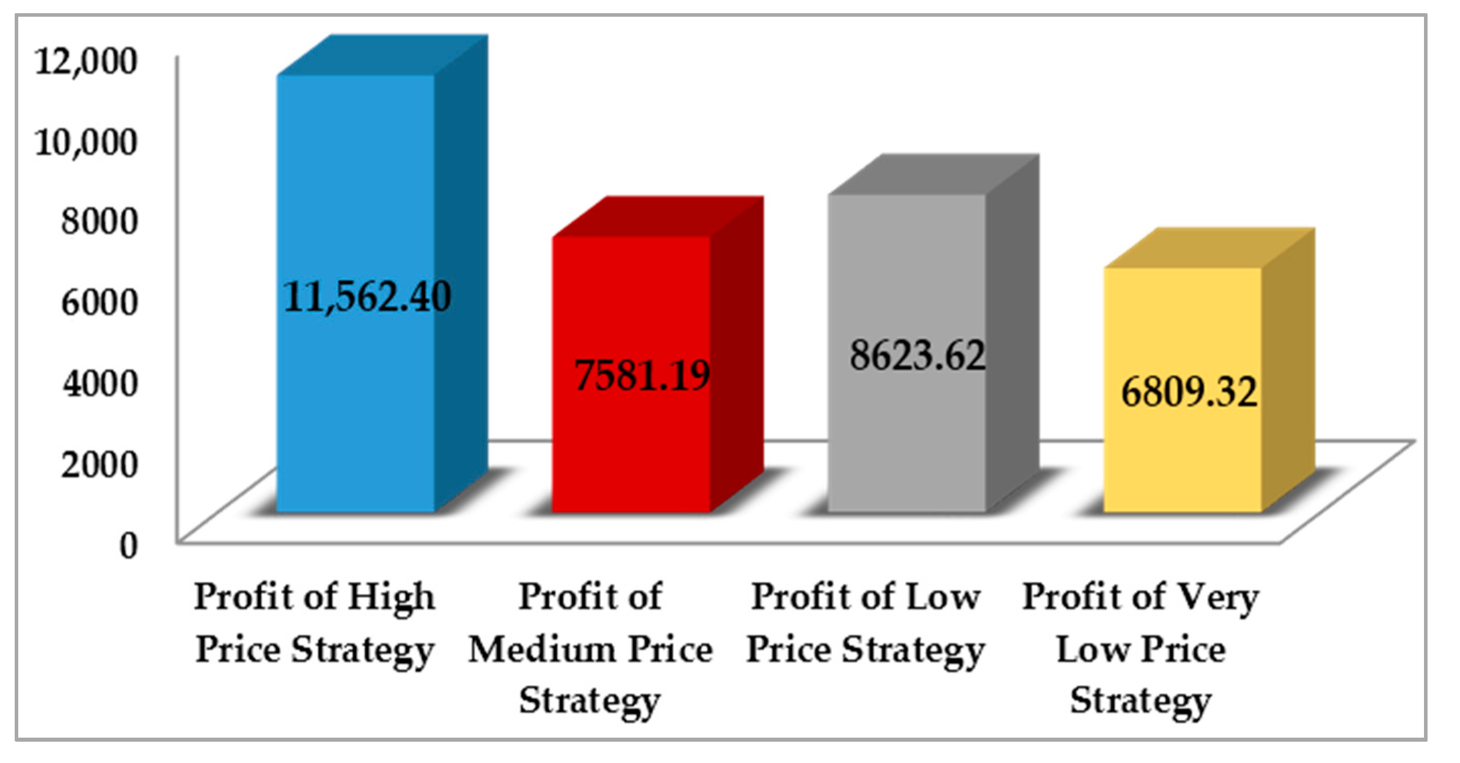
Although low prices and deep (very low) prices of the products are close, the methodologies are different. In addition, deep pricing strategy is just for big customers and applied occasionally when top management decides to use it. Consequently, the most profitable strategy for the supermarkets is low pricing scenario in
Figure 4, although small price variation between low and deep pricing is determined in the tables above.
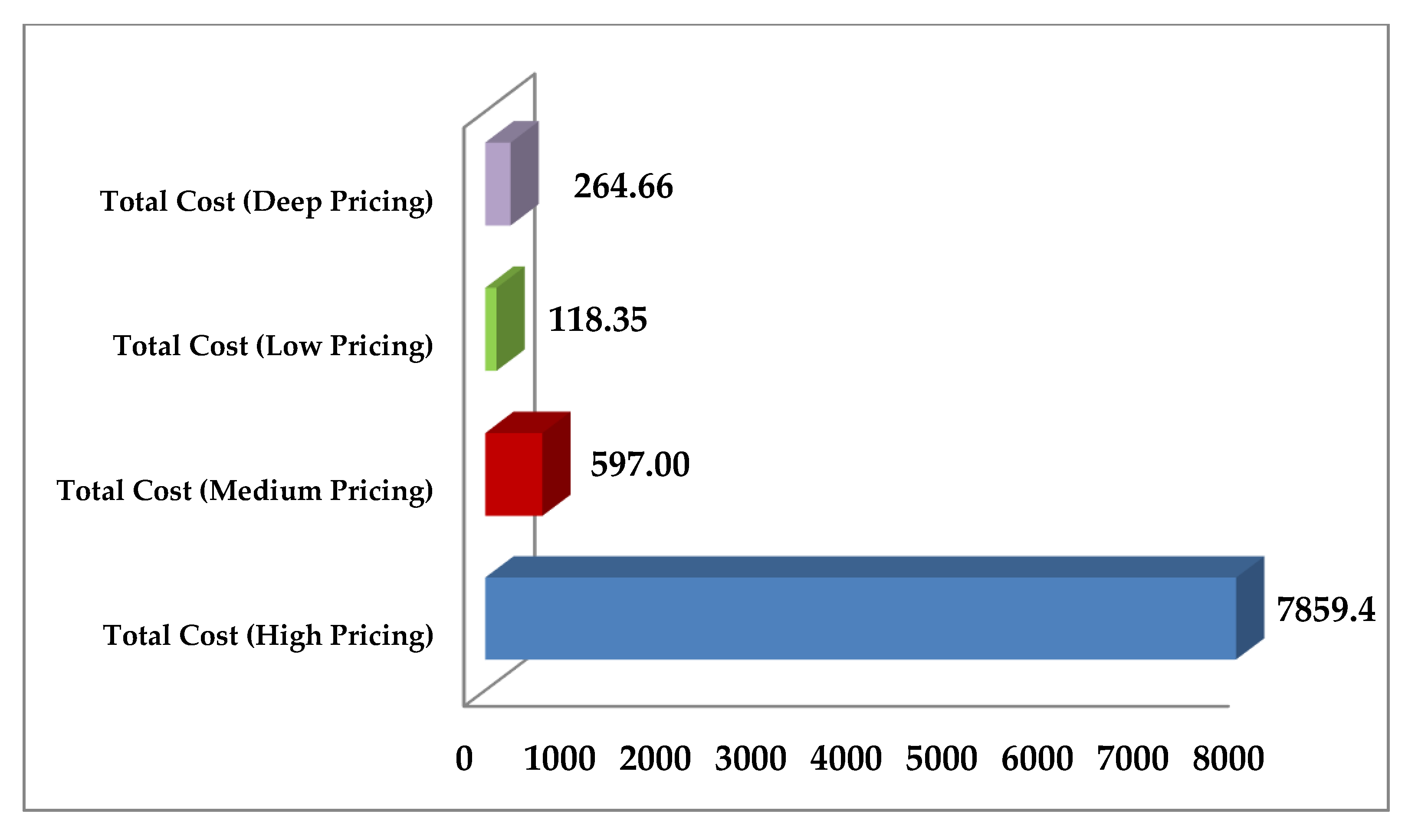
Furthermore, the differences between the common and the proposed systems for supermarkets are compared with each other. It is clearly determined in this paper that total profit of scenario 3 (low pricing strategy) is increased, while the total cost is decreased approximately 98.5% in the long term, as clearly seen in
Figure 5. However, more than 15% improvement is achieved for total profit via scenario 3. Moreover, numerical simulation results are defined with figures to show the effects of the proposed system in detail. It is clearly seen that although very low-price strategy is the most preferable strategy for the customers, it is not so useful for the supermarkets (because of profit balance). Therefore, low price based scenario is more profitable for both sustainable nature balance and sales sustainability in real life.


