Article

Land Development Suitability Evaluation of Pingtan Island Based on Scenario Analysis and Landscape Ecological Quality Evaluation

1
Third Institute of Oceanography, State Oceanic Administration, Xiamen 361005, China
2
Coastal and Ocean Management Institute, Xiamen University, Xiamen 361005, China
3
Island Research Center, State Oceanic Administration, Pingtan 350400, China
*
Author to whom correspondence should be addressed.
Sustainability 2017, 9(7), 1292; https://doi.org/10.3390/su9071292
Submission received: 31 May 2017 / Revised: 18 July 2017 / Accepted: 18 July 2017 / Published: 24 July 2017
(This article belongs to the Section Sustainable Urban and Rural Development)

Abstract

:
With the acceleration of urbanization and industrialization, regional development is becoming increasingly disordered. Thus, how to balance economic development and ecological protection is a key question. To comprehensively evaluate land development suitability, an evaluation index system for construction land and farmland suitability was established in this study based on natural and social-economic information. After selecting an island in China as the main case study in this work, the reference method was applied in grading and value assigning for all indices. In addition, the analytic hierarchy process and expert evaluation method were used to determine the index weighting. After scenario analysis was adopted in the study to analyze the impact of the policy orientation on the suitability evaluation, we finally evaluated the landscape ecological quality of different scenarios. Results showed the landscape ecological quality of a coordinated development scenario was the highest. The results indicated that coordinated development which takes the ecological protection and urban development into account may be a better choice for land planning.

1. Introduction

With the acceleration of urbanization and industrialization, a large amount of farmland and woodland have been occupied by urban and construction land. Regional development is becoming increasingly disordered, leading to resource overload and ecosystem destruction. The sustainability of regional development is threatened. How to balance economic development and ecological protection is the key to sustainable development [1,2,3]. Scientific and comprehensive land development evaluation has been recognized as being critical for assessing the land suitability for specific use and planning for future land use and management [4,5,6].
Land suitability evaluation is a process used to assess land suitability for a specific purpose [7], which can provide a comprehensive view for land development and planning and promote scientific and rational use of land resources [1,6,8,9,10,11,12]. For years, scientists have carried out many studies in land suitability evaluation. In the 1960s, land suitability evaluation procedures became the basis for land planning [13]. Since the 1970s, Geographical Information Technology has promoted the development of land suitability evaluation [8,9,14,15,16,17,18,19]. With advances in data collection and processing technology, land suitability evaluation has been gradually applied in various fields, such as crop suitability evaluation [20,21,22,23,24], landscape planning [25,26], waste management planning [27,28,29], environmental impact evaluation [30], land restoration [31], and urban sustainable development [32,33,34]. While few studies have considered the impact of policy orientation or development pattern on suitability evaluation, more attempts need to be made to evaluate land suitability in different scenarios.
In previous work, land suitability evaluation results in different scenarios have not been quantitatively evaluated. For example, Moreno compared the overall agreement between Boolean and fuzzy maps [35]. Elaalem and others made a comparison of the fuzzy analytic hierarchy process (AHP) and ideal point methods for evaluating land suitability [36]. However, few studies have quantitatively evaluated the results of different policy scenarios that place different levels of importance on economic and ecological impacts.
As the fifth-largest island in China, Pingtan was identified as a Comprehensive Experimental Zone by the Chinese government in 2010 [37]. Pingtan has developed quickly since then: urban construction sped up, reclamation projects increased significantly, tourism developed rapidly, and so on. The ecosystem of Pingtan Island (PI) is very fragile, with a lack of freshwater resources, increasing environmental pollution, and rapid vegetation decline. Land development suitability evaluation is therefore crucial for island-scale land use planning. Specifically, the research objectives of this study are: (1) to establish a land suitability index system, (2) to explore land development suitability in a rapid urbanization island in China under different development goals, (3) to evaluate the land development suitability result by using the landscape ecological quality (LEQ) method.

2. Materials and Methods

2.1. Study Area

PI is also known as Haitan Island, and is located in the northwest of the Taiwan Strait, with an area of about 300 km2, and consists of 11 towns: Tancheng, Suao, Liushui, Aoqian, Beicuo, Pingyuan, Aodong, Baiqing, Luyang, Zhonglou, and Lancheng (Figure 1). The north and south of PI are hills and plateaus, while the middle is a plain. As the largest island of Fujian Province, PI is situated in a subtropical zone with a monsoon climate, with annual average rainfall of 900–1200 mm. The central plain is agricultural, with farmlands of peanuts, sweet potatoes, and vegetables. PI was designated as a Special Zone in 2010 to attract investment with tax relief and favorable land development policies. PI has constituted one of China’s fastest developing regions in terms of rapid industrialization and urbanization, with large areas of fragile natural ecosystems faced with great damage.

2.2. Methods

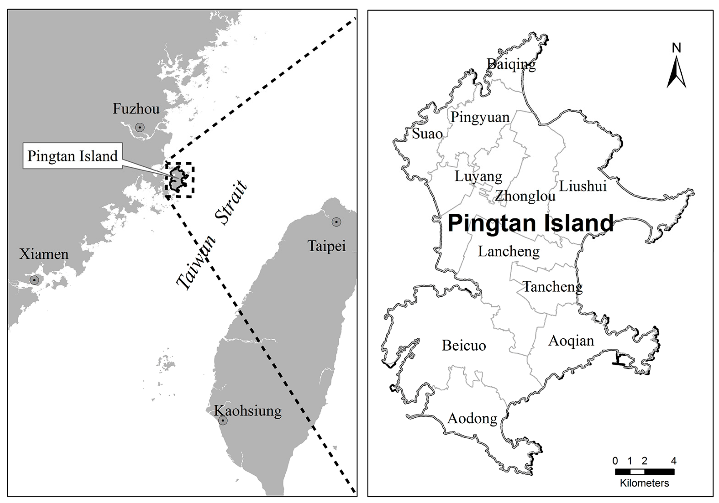
2.2.1. Factors Used in the Land Suitability Analysis

To determine whether the land that has not been developed for construction or farming is suitable for these purposes, the factors of elevation, slope, traffic condition, vegetation, soil erosion, and water resource were used (Table 1). The main reasons for using these factors in this study were that the spatial data concerning the factors used had already been made available for use and the factors used in the study are adequate for determining the areas where agricultural production or urban construction can be carried out. The factors used in this study are explained in detail in the following sections.
Elevation is an important factor that plays a role in the variation of plant cover by causing water resource and soil changes. The higher the elevation, the less water there is [38]. It is difficult to store rainwater or utilize groundwater on the hills of PI. Field surfaces on hills are full of stone, which is difficult for agriculture or construction, while in the plains, the soil is suitable for agriculture. In most places with high elevation, transportation is inconvenient, which is also unsuitable for construction.
Slope limits agricultural production by affecting soil properties. The thickness of the soil layer decreases with increasing slope. Slope degree is the main factor determining erosion control [39,40]. Accordingly, with an increase in slope degree, the development of soils occurs slowly, and soil depth and fertility decrease. Slope negatively affects urban construction by restricting the possibility of using machines and human activity. On the other hand, urban construction will create more bare land, the erosion of which will increase with the increase of the slope degree.
Traffic conditions represent a spatial association between new construction land and existing urban land. The distance to roads increases with decreasing connection and convenience. Traffic conditions have also been used in many other studies [41,42,43].
Vegetation is important for ecosystem stability, and a high vegetation index represents high biomass and biodiversity, so the development cost is increased with increasing vegetation. The normalized difference vegetation index (NDVI) has a long history of use in remote sensing, ecology, and geography to study vegetation characteristics including amount, type, and condition [44,45,46]. The NDVI is a reflection of the biophysical conditions of island vegetation cover. We explored NDVI from Landsat Thematic Mapper (TM) satellite imagery.
Soil erosion reduces the soil depth, which is necessary for the development of plant roots and the amount of water that the plants need, decreasing the content of nutritional elements and organic matter [47,48]. Erosion is connected with soil properties. The suitability of the soil for agriculture decreases with the increasing erosion modulus.
Water resource is another important factor for agriculture. Water is the foundation of agriculture. Agriculture increases pressure on the water supply, so water is the limiting condition for agriculture. The annual average runoff depth was selected to represent water resource in our study.

2.2.2. AHP Method

AHP is a multi-criteria decision-making approach introduced by Saaty [49,50] which enables users to determine the weights of the factors in the solution of a multi-criteria problem. In the AHP method, a hierarchical model consisting of objectives, criteria, sub-criteria, and alternatives is used for every problem [51]. After the problem is set on a hierarchical structure, the weights of the criteria forming the hierarchy are calculated. To evaluate the criteria included in a level compared with other criteria included in the next hierarchy level, scoring is made with the utilization of the preference scale (Table 2) [52], and a pairwise comparison matrix was created to compare one factor with another [52,53].
The AHP approach involves the following five steps: (1) developing an AHP decision model tree; (2) determining the relative importance of a factor to other factors in the judgment matrix; (3) conducting a consistency validation of the judgment matrix forms; (4) calculating the relative importance of each factor and weighting the overall ratings of every layer; and (5) giving a score to each factor based on the score index system. The maximum of the eigenvalue and its eigenvector should be calculated and verified by the coherence ratio (CR). The CR value should be less than 0.10, otherwise the matrix must be adjusted once again [10,52,54]. The pairwise comparison matrix was created to determine the weights of factors (Table 3 and Table 4). The relative importance of a factor to other factors was determined by consulting the opinions of a team of experts, including local residents, officials, and experts engaging in geography, oceanography, and ecological research.

2.2.3. Scenario Analysis (SA)

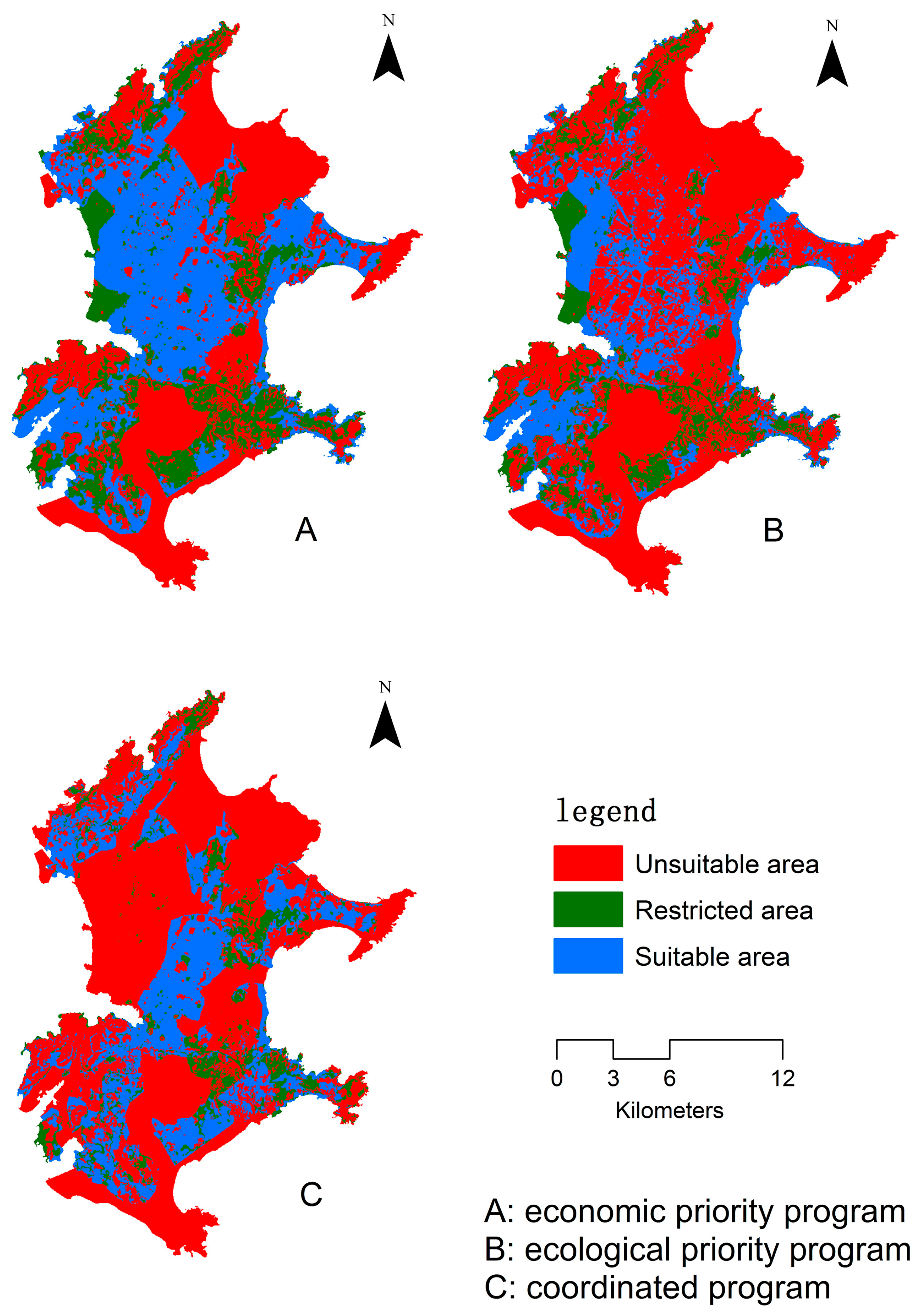
In addition to the basic suitability evaluation factors, factors that affect the island land security should be considered in order to protect the ecological security and construction land of the island. In our study, we took scenic areas and protected areas as ecologically sensitive areas. After construction land and farmland suitability evaluation, we proposed three different land suitability evaluation programs of the island based on different development goals, which are as follows:
(1) Economic priority program
This program focuses on economic development. The program is based on a construction land suitability evaluation, taking existing construction land and ecologically sensitive areas as the unsuitable zone.
(2) Ecological priority program
This program focuses on ecological protection. The program is based on construction land suitability evaluation, taking existing construction land, ecologically sensitive areas, and farmland as the unsuitable zone.
(3) Coordinated development program
Without prejudice to the island’s ecological security, this program can meet the demand for the city’s construction as much as possible. Thus, after deducting the ecologically sensitive areas and existing construction land, we put forward the principle of coordinated development [55,56], as shown in Table 5. In the principle of coordinated development, when the land is suitable for agriculture, it is unsuitable for development, because farmland needs protection. When the land is unsuitable for construction, it is also unsuitable for development. When the land is suitable or restrictive for construction and unsuitable for agriculture, it is suitable for development. When the land is suitable for construction and restrictive for agriculture, it is suitable for development. When the land is restrictive for construction agriculture, it is restrictive for development.

2.2.4. LEQ Evaluation Method

(1) LEQ evaluation
LEQ refers to the ability of a landscape’s ecosystem to maintain its structure and functional stability, taking landscape ecosystem stability as a measure. The stability of LEQ depends on the degree of stability and disturbance of the landscape ecosystem. If the disturbance level of LEQ is greater than the stability, the landscape ecosystem tends toward being unsteady, and LEQ is low; Otherwise, the landscape ecosystem is stable, and LEQ is high [57].
In this study, the Equation (1) was used to evaluate LEQ, which is shown as follows:
V = Vw/Vg
where V represents LEQ, Vg is the landscape disturbance index, and Vw is the landscape stability index. The higher the V value, the higher the LEQ. Landscape disturbance index and landscape stability index will be described below.
(2) Landscape disturbance index and landscape stability index
The landscape disturbance is affected by landscape fragmentation and land use activities. Landscape fragmentation is a major cause of biodiversity loss, and human activities block the migration of biology and flow of material and energy [30,57]. In our study, the landscape shape index (LSI), patch density (PD), and the ratio of construction land (CI) were selected to characterize the landscape disturbance [57,58,59,60,61]. LSI is used to indicate the development of patches and the complexity of patch borders. Higher LSI value indicates higher degree of landscape fragmentation, which is related to higher landscape disturbance. PD refers to the fragmentation of the landscape, indicating human disturbance intensity [62]. Higher PD value means higher landscape disturbance. CI means the construction area proportion of the total landscape area. Higher CI value indicates higher landscape disturbance. In this study, we assumed that the suitable development area was construction land. We also assumed that LSI, PD, and CI have the same contribution to landscape disturbance.
Landscape stability depends on the structure of land use, biodiversity, and landscape aggregation [57]. Different land use makes different contributions to landscape stability. Wetlands are the best, woodlands next, followed by arable land and water. Construction land is the worst. In this study, suitability evaluation results were used to represent the land use: we identify unsuitable zones as 3, restrictive zones as 2, and suitable zones as 1 quantitatively. Land use contributions to landscape stability were multiplied by the proportion of land use, then weighted to the land use structure index (LS). Higher LS value means higher landscape stability. The vegetation index (VI) is an important factor that affects landscape ecological stability, characterized by the ratio of the area that is covered by vegetation. Higher VI indicates higher landscape stability. In this study, we assumed that unsuitable zone was completely covered by vegetation, half of the restricted area was covered by vegetation, and the suitable zone was uncovered. Optimized landscape patterns are helpful for landscape stability [57], and the landscape contagion index (CONT) was selected to describe the agglomeration of different types of patches. Higher CONT value means higher landscape stability. We assumed that LS, VI, and CONT have the same contribution to landscape stability.
Landscape disturbance index is evaluated by LSI, PD, and CI. The Equation (2) is as follows:
Vg = (x1 + x2 + x3)/3
where Vg is the landscape disturbance index, x1 is the LSI, x2 is the PD, x3 is the CI.
Landscape stability index is evaluated by LS, CONT, and VI. The Equation (3) is as follows:
Vw = (x4 + x5 + x6)/3
where Vw is the landscape stability index, x4 is the LS, x5 is the VI, x6 is the CONT.
The indices x1 to x6 are described in Table 6. All the indices should be standardized, and all these values ranged from 0 to 1.

2.2.5. Data Sets and Methodology

The slope and elevation data were obtained from the GRID digital elevation model (DEM, CNIC, Beijing, China) of the study area, and the DEM was downloaded from Geospatial Data Cloud [58]. The cell size of slope and elevation map was 30 × 30 m.
The 30 × 30 m cell size ESRI GRID (ESRI, Redlands, CA, USA) format NDVI map (vegetation index) of the study area were generated from the Landsat Thematic Mapper (USGS, Reston, VA, USA) satellite imagery of 2013 with 30 m resolution. Twenty-one ground control points were used, and the root mean square errors were less than 0.5 pixels. The image was re-sampled to 30 m resolution.
The main road map of 2010 was digitized from 1/200,000 printed map obtained from the Traffic Bureau of Pingtan. The 30 × 30 m cell size ESRI GRID format traffic index map of the study area was generated from ESRI Shape format road map by using the Euclidean distance normalization method.
The ESRI Shape format soil erosion map of 2013 was digitized from 1/200,000 printed map obtained from the Land and Resources Bureau of Pingtan, and the ESRI Shape format water resource index map was digitized from the water resource map in Pingtan water resources allocation planning report [59]. The ESRI Shape format maps were converted into ESRI GRID format maps with 30 m resolution.
All GIS layers were transformed into the same coordinate system and projection; that is, the projection is Transverse Mercator, the central meridian is 120° E, and the Ellipsoid is WGS 1984. The cell size of ESRI GRID format layers were 30 × 30 m. All the indices were standardized to a uniform rating scale. The class boundaries and standardized measurements are given in 
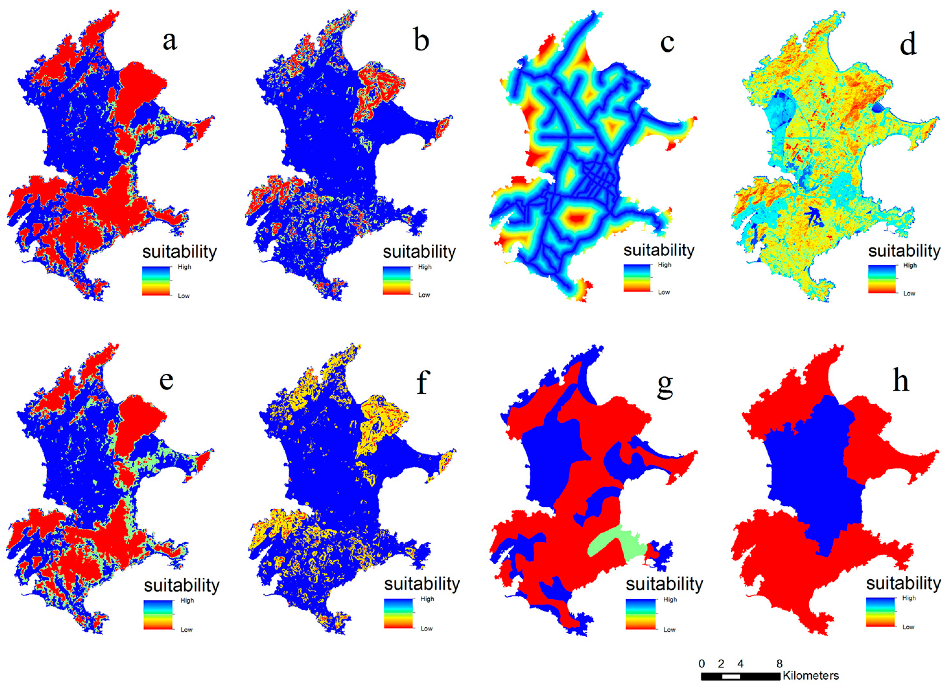
Table 1, and the spatial pattern maps are shown in Figure 2.
After the weights of factors were determined according to the AHP method, factors weights and factors scores were appointed to the related layers in the ArcGIS 10.1 environment, raster maps of eight factors were overlaid using the weighted sum overlay analysis, and a construction land suitability map and a farmland suitability map were generated. The analysis layers (construction land suitability map and farmland suitability map) were divided into three classes according to natural breaks in the ArcGIS 10.1 environment. The highest score area was identified as suitable area, which was followed by restrictive area. The lowest score area was identified as unsuitable area.
The land suitability map of the economic priority program was obtained by identifying existing construction land and ecologically sensitive areas as the unsuitable zone based on the construction land suitability map. The land suitability map of the ecological priority program was obtained by identifying existing construction land, ecologically sensitive areas, and farmland as the unsuitable zone based on the construction land suitability map. The land suitability map of coordinated development program was obtained according to the principle shown in Table 5 based on the construction land suitability map and farmland suitability map. Then, the ecologically sensitive areas and existing construction land were taken as the unsuitable zone. The above processes were implemented in the arcGIS 10.1 environment by raster calculation and reassignment.
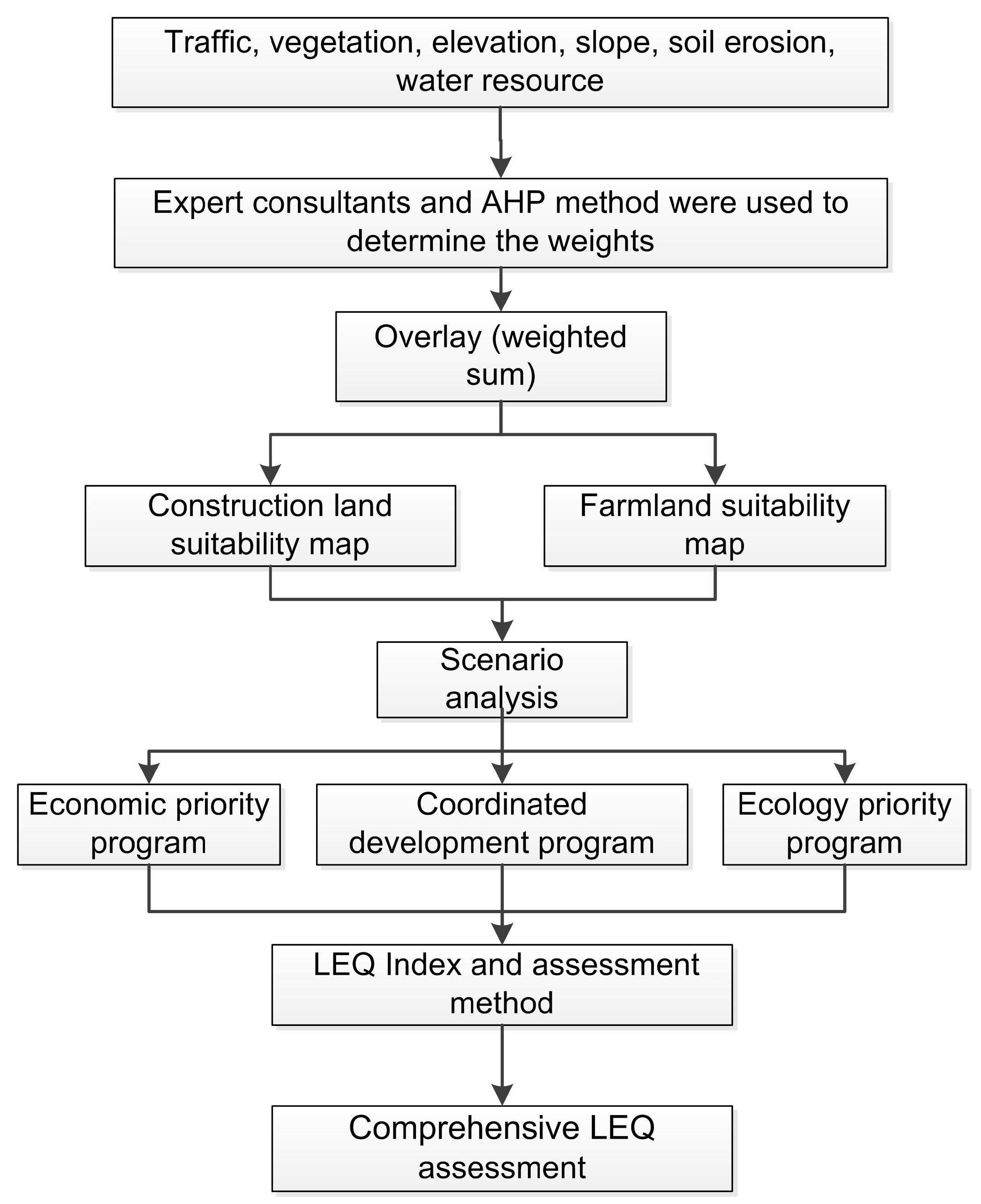
The six indices in the LEQ evaluation (LSI, PD, CI, LS, VI, and CONT) were calculated by Fragstats 4.2 (UMASS, Amherst, USA) based on land suitability map for three scenarios. Then, we calculated the landscape disturbance index, landscape stability index, and LEQ index according to Equations (2), (3), and (1), respectively. The steps followed in this study are presented in general terms in Figure 3.

3. Results

3.1. Land Development Suitability Evaluation

For the three scenarios, the unsuitable zone areas were the largest, followed by suitable zone, while the restricted zone areas were the smallest. The suitable zone was mainly located in the central plains of PI, and the unsuitable zone was mainly in the mountainous areas and urban built-up areas (Figure 4).
The percentage of the suitable zone in the economic priority program was the largest among the three scenarios, while the percentage in the ecological priority program was the lowest. For restricted zones, the largest was the economic priority program and the lowest was the coordinated program. The percentage of unsuitable zone in economic priority program was the lowest, while that in the coordinated program was the largest (Table 7).

3.2. LEQ Evaluation

For landscape disturbance, CI was the highest in the economy priority program, indicating that the landscape was affected by construction land in the economic priority program. LSI and PD were highest in the ecological priority program, indicating that the patch shape was most irregular, and the fragmentation degree was the highest. However, CI was minimal in this program. LSI, PD, and CI were at a medium level in the coordinated program, and the landscape disturbance index was minimal (Table 8).
The landscape stability index score of the coordinated program was the highest. LS of economic priority program was the highest, while VI and CONT were the lowest, indicating that LS has a higher contribution to LEQ. In the ecology priority program, VI was the highest, and CONT was at a medium level. The CONT and VI in the coordinated program were high (Table 8), indicating that the landscape was dominated by a few large patches or the same type of patch was highly connected, which was good for intensive use of the land.
A comprehensive evaluation of LEQ showed that the score of the coordinated program was the highest, followed by the economic priority program, and the ecology priority program was the lowest. In the economic priority program, the landscape disturbance and stability were both the lowest, and LEQ was at a medium level. In the ecological priority program, the landscape disturbance was at the highest level, while stability was at a medium level, so LEQ was the lowest (Table 8). The coordinated program had lowest landscape disturbance while having the highest stability, and the highest LEQ.

4. Discussion

4.1. Spatial Variation of Land Development Suitability

Land development suitability evaluation results showed that the suitable zone was mainly distributed in the plain, but the unsuitable zone was mainly distributed in hilly areas. This is similar to other findings [41,60]. The hills comprise high altitude and slope, which not only directly affects construction and cultivation, but also affects transportation, soil, and water resources that are related to construction and cultivation [40]. The coastal area in PI was an unsuitable zone, which is useful for ecological integrity and landscape connectivity, and helpful for forming the ecological barrier of PI [37,61].

4.2. SA of Land Development Suitability

Rapid urbanization promoted economic development, but damaged the ecosystem. How to balance the two aspects is a relevant and difficult problem [1,2,3,43,61]. In our study, both economic development and ecological protection were considered in SA. The LEQ of the coordinated development scenario is the highest, which is similar to the results of other studies [43]. The result showed that from the perspective of landscape ecology, pure urban development or ecological protection may be inappropriate, not meeting the needs for integrated development. However, coordinated development may be a better choice, which takes both the ecological protection and urban development into account. The use of SA allows several decision scenarios to be evaluated in order to guide managers or planners to reach the most satisfactory solution considering trade-off measures involved in the decision-making process.

4.3. Landscape Ecological Evaluation Method of Land Development Suitability

Different development scenarios have different landscape effects, so landscape evaluation provides a quantitative tool for evaluating the results of different scenarios. In this study, from the perspective of landscape ecosystem structure and function, a landscape ecological multi-parameter evaluation system was established to quantitatively analyze land suitability.
PD characterizes landscape fragmentation. High PD means a high degree of landscape fragmentation, which is usually caused by a high intensity of human disturbance. A higher LSI value indicates longer and irregular borders, which also means a higher degree of landscape fragmentation [62,63,64,65,66,67,68]. Human activities including urban construction, rural residential, and traffic construction block the migration of biology and the movement of material and energy [31,57]. When the ratio of interference in an area increases, the landscape stability tends to decrease [69,70].
Increased vegetation coverage is conducive to biological migration, environment improvement, habitat protection, and landscape stability. Vegetation coverage in an unsuitable zone is higher than the suitable and restricted zones, and therefore has a greater contribution to LEQ. The CONT index describes the contagion of landscapes. CONT is close to zero when the dispersion degree is the highest. When the patch is completely gathered, CONT equals 100. Increased CONT indicates an increased degree of contagion [67,68,71,72].

5. Conclusions

This study uses GIS, AHP, SA, and LEQ to evaluate the land development suitability under the pressure of economic development and ecological protection on an island. The suitable zone was mainly distributed in the plain, and the unsuitable zone was mainly distributed in hilly areas, which reflects that high altitudes and slope affected transportation, soil, and water resources related to construction and cultivation. The coordinated program had the highest LEQ score, indicating that pure urban development or ecological protection may be inappropriate, while coordinated development may be a better choice. SA could guide managers or planners to reach the most satisfactory solution taking into account trade-off measures involved in the decision-making process.

Acknowledgments

The research was funded by the National Natural Science Foundation of China (Grant No. 41406121) and the Scientific Research Foundation of Third Institute of Oceanography, State Oceanic Administration (Grant No. 2012020).

Author Contributions

Qingsheng Li conceived and designed this research; Qingsheng Li, Jinliang Huang, Cui Wang and Heshan Lin conducted the model building and the results discussion; Qingsheng Li, Cui Wang and Heshan Lin performed the data collection and calculation; Qingsheng Li, Jinliang Huang and Jinlong Jiang contributed to the comparison and discussion, and wrote the paper; and Jiwei Zhang and Bingkun Wang provided important advice for paper promotion.

Conflicts of Interest

The authors declare no conflict of interest.

References

  1. Collin, M.L.; Melloul, A.J. Combined land-use and environmental factors for sustainable groundwater management. Urban Water 2001, 3, 229–237. [Google Scholar] [CrossRef]
  2. Styers, D.M.; Chappelka, A.H.; Marzen, L.J.; Somers, G.L. Developing a land-cover classification to select indicators of forest ecosystem health in a rapidly urbanizing landscape. Landsc. Urban Plan. 2010, 94, 158–165. [Google Scholar] [CrossRef]
  3. Zhang, J.; Fu, M.; Zhang, Z.; Tao, J.; Fu, W. A trade-off approach of optimal land allocation between socio-economic development and ecological stability. Ecol. Model. 2014, 272, 175–187. [Google Scholar] [CrossRef]
  4. Joerin, F.; Theriault, M.; Musy, A. Using GIS and outranking multicriteria analysis for land-use suitability evaluation. Int. J. Geogr. Inf. Sci. 2001, 15, 153–174. [Google Scholar] [CrossRef]
  5. Malczewski, J. GIS-based land-use suitability analysis: A critical overview. Prog. Plan. 2004, 62, 3–65. [Google Scholar] [CrossRef]
  6. Shearer, K.S.; Xiang, W.N. Representing multiple voices in landscape planning: A land suitability evaluation study for a park land-banking program in Concord, North Carolina, USA. Landsc. Urban Plan. 2009, 93, 111–122. [Google Scholar] [CrossRef]
  7. Steiner, F.; McSherry, L.; Cohen, J. Land suitability analysis for the Upper Gila River Watershed. Landsc. Urban Plan. 2000, 50, 199–214. [Google Scholar] [CrossRef]
  8. Bojórquez-Tapia, L.A.; Diaz-Mondragón, S.; Ezcurra, E. GIS-based approach for participatory decision making and land suitability evaluation. Int. J. Geogr. Inf. Sci. 2001, 15, 129–151. [Google Scholar] [CrossRef]
  9. Malczewski, J. Ordered weighted averaging with fuzzy quantifiers: GIS-based multicriteria evaluation for land-use suitability analysis. Int. J. Appl. Earth Obs. 2006, 8, 270–277. [Google Scholar] [CrossRef]
  10. Chen, H.; Liu, G.; Yang, Y.; Ye, X.; Shi, Z. Comprehensive Evaluation of Tobacco Ecological Suitability of Henan Province Based on GIS. Agric. Sci. China 2010, 9, 583–592. [Google Scholar] [CrossRef]
  11. Chen, Y.; Yu, J.; Khan, S. Spatial sensitivity analysis of multi-criteria weights in GIS-based land suitability evaluation. Environ. Modell. Softw. 2010, 25, 1582–1591. [Google Scholar] [CrossRef]
  12. Gallant, A.L.; Euliss, J.N.H.; Browning, Z. Mapping Large-Area Landscape Suitability for Honey Bees to Assess the Influence of Land-Use Change on Sustainability of National Pollination Services. PLoS ONE 2014, 9, e99268. [Google Scholar] [CrossRef] [PubMed]
  13. McHarg, I.L. Design with Nature; Natural History Press: Garden City, NY, USA, 1969. [Google Scholar]
  14. Bauer, K.W. The use of soils data in regional planning. Geoderma 1973, 10, 1–26. [Google Scholar] [CrossRef]
  15. Fabos, J.G.Y.; Greene, C.M.; Joyner, S.A. The Metland Landscape Planning Process: Composite Landscape Evaluation, Alternative Plan Formulation, and Plan Evaluation; Massachusetts Agricultural Experiment Station, University of Massachusetts: Amherst, MA, USA, 1978. [Google Scholar]
  16. Wandahwa, P.; Van Ranst, E. Qualitative land suitability evaluation for pyrethrum cultivation in west Kenya based upon computer-captured expert knowledge and GIS. Agric. Ecosyst. Environ. 1996, 56, 187–202. [Google Scholar] [CrossRef]
  17. Ahamed, T.R.N.; Rao, K.G.; Murthy, J.S.R. GIS-based fuzzy membership model for crop-land suitability analysis. Agric. Syst. 2000, 63, 75–95. [Google Scholar] [CrossRef]
  18. Mendas, A.; Delali, A. Integration of MultiCriteria Decision Analysis in GIS to develop land suitability for agriculture: Application to durum wheat cultivation in the region of Mleta in Algeria. Comput. Electron. Agric. 2012, 83, 117–126. [Google Scholar] [CrossRef]
  19. Reshmidevi, T.V.; Eldho, T.I.; Jana, R.A. GIS-integrated fuzzy rule-based inference system for land suitability evaluation in agricultural watersheds. Agric. Syst. 2009, 101, 101–109. [Google Scholar] [CrossRef]
  20. Wang, D.; Li, C.; Song, X.; Wang, J.; Yang, X.; Huang, W.; Wang, J.; Zhou, J. Evaluation of Land Suitability Potentials for Selecting Winter Wheat Cultivation Areas in Beijing, China, Using RS and GIS. Agric. Sci. China 2011, 10, 1419–1430. [Google Scholar] [CrossRef]
  21. Yu, J.; Chen, Y.; Wu, J.; Khane, S. Cellular automata-based spatial multi-criteria land suitability simulation for irrigated agriculture. Int. J. Geogr. Inf. Sci. 2011, 25, 131–148. [Google Scholar] [CrossRef]
  22. Liu, Y.; Jiao, L.; Liu, Y.; He, J. A self-adapting fuzzy inference system for the evaluation of agricultural land. Environ. Modell. Softw. 2013, 40, 226–234. [Google Scholar] [CrossRef]
  23. Yalew, S.G.; Van Griensven, A.; Van der Zaag, P. AgriSuit: A web-based GIS-MCDA framework for agricultural land suitability evaluation. Comput. Electron. Agric. 2016, 128, 1–8. [Google Scholar] [CrossRef]
  24. Kong, C.; Lan, H.; Yang, G.; Xu, K. Geo-environmental suitability evaluation for agricultural land in the rural–urban fringe using BPNN and GIS: A case study of Hangzhou. Environ. Earth Sci. 2016, 75, 1136. [Google Scholar] [CrossRef]
  25. Uy, P.D.; Nakagoshi, N. Application of land suitability analysis and landscape ecology to urban greenspace planning in Hanoi, Vietnam. Urban For. Urban Green. 2008, 7, 25–40. [Google Scholar] [CrossRef]
  26. Pourebrahim, S.; Hadipour, M.; Mokhtar, M.B.; Mohamed, M.I.H. Analytic network process for criteria selection in sustainable coastal land use planning. Ocean Coast. Manag. 2010, 53, 544–551. [Google Scholar] [CrossRef]
  27. Aragonés-Beltrán, P.; Pastor-Ferrando, J.P.; García-García, F.; Pascual-Agulló, A. An Analytic Network Process approach for siting a municipal solid waste plant in the Metropolitan Area of Valencia (Spain). J. Environ. Manag. 2010, 91, 1071–1086. [Google Scholar] [CrossRef] [PubMed]
  28. Baiocchi, V.; Lelo, K.; Polettini, A.; Pomi, R. Land suitability for waste disposal in metropolitan areas. Waste Manag. Res. 2014, 32, 707–716. [Google Scholar] [CrossRef] [PubMed]
  29. Chang, N.; Parvathinathan, G.; Breeden, J.B. Combining GIS with fuzzy multicriteria decision-making for landfill siting in a fast-growing urban region. J. Environ. Manag. 2008, 87, 139–153. [Google Scholar] [CrossRef] [PubMed]
  30. Marull, J.; Mallarach, J.M. A new GIS methodology for assessing and predicting landscape and ecological connectivity: Applications to the metropolitan area of Barcelona (Catalonia Spain). Landsc. Urban Plan. 2005, 71, 243–262. [Google Scholar] [CrossRef]
  31. Wang, S.; Liu, C.; Zhang, H. Suitability evaluation for land reclamation in mining area: A case study of Gaoqiao bauxite mine. Trans. Nonferrous Met. Soc. China 2011, 21, 506–515. [Google Scholar] [CrossRef]
  32. Xu, K.; Kong, C.; Li, J.; Zhang, L.; Wu, C. Suitability evaluation of urban construction land based on geo-environmental factors of Hangzhou, China. Comput. Geosci. 2011, 37, 992–1002. [Google Scholar] [CrossRef]
  33. Cerreta, M.; Toro, P.D. Urbanization suitability maps: A dynamic spatial decision support system for sustainable land use. Earth Syst. Dyn. 2012, 3, 157–171. [Google Scholar] [CrossRef] [Green Version]
  34. Malmir, M.; Zarkesh, M.M.K.; Monavari, S.M.; Jozi, S.A.; Sharifi, E. Analysis of land suitability for urban development in Ahwaz County in southwestern Iran using fuzzy logic and analytic network process (ANP). Environ. Monit. Assess. 2016, 188, 447. [Google Scholar] [CrossRef] [PubMed]
  35. Moreno, J. Applicability of knowledge-based and fuzzy theory-oriented approaches to land suitability for upland rice and rubber, as compared to the farmers’ perception: A case study of Lao PDR. Unpublished Master’s Thesis, International Institute for Geo-Information Science and Earth Observation, Enschede, The Netherlands, 2007. [Google Scholar]
  36. Elaalem, M.; Comber, A.; Fisher, P. A Comparison of Fuzzy AHP and Ideal Point Methods for Evaluating Land Suitability. Trans. GIS 2011, 15, 329–346. [Google Scholar] [CrossRef]
  37. Li, Q.; Huang, J.; Wang, C.; Wang, B.; Wu, Y.; Zhang, J.; Lin, H.; Luo, H. Assessment of the Pingtan Island land development suitability based on comprehensive ecological–economic–industrial analysis. Mar. Sci. 2017, 41, 1–10. [Google Scholar]
  38. Akinci, H.; Ozalp, A.Y.; Turgut, B. Agriculture land use suitability analysis using GIS and AHP technique. Comput. Electron. Agric. 2013, 97, 71–82. [Google Scholar] [CrossRef]
  39. Datye, V.S.; Gupte, S.C. Association between agricultural land use and physico-socio-economic phenomena: A multivariate approach. Trans. Inst. Ind. Geogr. 1984, 6, 61–72. [Google Scholar]
  40. Koulouri, M.; Giourga, C. Land abandonment and slope gradient as key factors of soil erosion in Mediterranean terraced lands. Catena 2007, 69, 274–281. [Google Scholar] [CrossRef]
  41. Park, S.; Jeonb, S.; Kim, S.; Choi, C. Prediction and comparison of urban growth by land suitability index mapping using GIS and RS in South Korea. Landsc. Urban Plan. 2011, 99, 104–114. [Google Scholar] [CrossRef]
  42. Gong, J.; Liu, Y.; Chen, W. Land suitability evaluation for development using a matter-element model: A case study in Zengcheng, Guangzhou, China. Land Use Policy 2012, 29, 464–472. [Google Scholar] [CrossRef]
  43. Liu, Y.; Peng, J.; Han, Y.; Wei, H.; Du, Y. Suitability evaluation for building land consolidation on gentle hillside based on OWA operator: A case in Dali Bai Nationality Borough in Yunnan, China. Acta Ecol. Sin. 2014, 34, 3188–3197. [Google Scholar]
  44. Lauver, C.; Whistler, J. A hierarchical classification of Landsat TM imagery to identify natural grassland areas and rare species habitat. Photogramm. Eng. Remote Sens. 1993, 60, 627–634. [Google Scholar]
  45. Jensen, J. Introduction to Digital Image Processing; Prentice Hall: Upper Saddle River, NJ, USA, 1996. [Google Scholar]
  46. Rundquist, B.C.; Harrington, J.A., Jr.; Goodin, D.G. Meso scale satellite bioclimatology. Prof. Geogr. 2000, 52, 331–344. [Google Scholar] [CrossRef]
  47. Lobo, D.; Lozano, Z.; Delgado, F. Water erosion risk evaluation and impact on productivity of a Venezuelan soil. Catena 2005, 64, 297–306. [Google Scholar] [CrossRef]
  48. Ziadat, F.M.; Sultan, K.A. Combining current land use and farmers’ knowledge to design land-use requirements and improve land suitability evaluation. Renew. Agric. Food Syst. 2011, 26, 287–296. [Google Scholar] [CrossRef]
  49. Saaty, T.L. A scaling method for priorities in hierarchical structures. J. Math. Psychol. 1977, 15, 57–68. [Google Scholar] [CrossRef]
  50. Saaty, T.L. Fundamentals of Decision Making and Priority Theory with the AHP; RWS Publications: Pittsburgh, PA, USA, 1994. [Google Scholar]
  51. Saaty, T.L. An exposition of the AHP in reply to the paper remarks on the analytic hierarchy process. Manag. Sci. 1990, 36, 259–268. [Google Scholar] [CrossRef]
  52. Saaty, T.L. The Analytic Hierarchy Process: Planning, Priority Setting, Resource Allocation; McGraw-Hill International: New York, NY, USA, 1980. [Google Scholar]
  53. Saaty, T.L. Mathematical Methods of Operations Research; Dover Publications: Mineola, NY, USA, 2004. [Google Scholar]
  54. Carrion, J.A.; Estella, A.E.; Dols, F.A.; Toro, M.Z.; Rodriguez, M.; Ridao, A.R. Environmental decision-support systems for evaluating the carrying capacity of land areas: Optimal site selection for grid-connected photovoltaic power plants. Renew. Sustain. Energy Rev. 2008, 12, 2358–2380. [Google Scholar] [CrossRef]
  55. Lu, Y.; Zong, Y. Ecological Planning of Land Use: The Central Area of Tianjin. J. Environ. Sci. China 1996, 25, 421–424. [Google Scholar]
  56. Ju, J. A Primary Integration Matrices Approach to Sustainability Orientated Land Use Planning; Institute of Regional Development Planning: Stuttgart, Germany, 1998. [Google Scholar]
  57. Zhu, Y.; Pu, L.; Zhao, C. Evaluation of Landscape Ecological Quality—A Case Study in Wujing County. Sci. Geogr. Sin. 2007, 27, 182–187. [Google Scholar]
  58. Computer Network Information Center, Chinese Academy of Sciences. Geospatial Data Cloud. 2014. Available online: http://www.gscloud.cn/ (accessed on 25 June 2016). (In Chinese)
  59. Chen, W.; Zhan, Y. Pingtan Water Resources Allocation Planning Report; Fujian Provincial Investigation Design & Research Institute of Water Conservancy & Hydropower: Fuzhou, China, 2010. [Google Scholar]
  60. Lei, S.; Hao, J.; Wang, L. Evaluation of exploitation suitability of unutilized arable lands in ecologically fragile areas—A case study of Datong City, Shanxi Province. Chin. J. Eco-Agric. 2011, 19, 1417–1423. [Google Scholar]
  61. Jiao, S.; Li, Z.; Gao, Q.; Zhou, K.; Wei, C.; He, S. The application of landscape connectivity theory in urban ecology suitability evaluation and optimization. Geogr. Res. 2013, 32, 720–730. [Google Scholar]
  62. Turner, M.G.; Ruscher, C.L. Changes in landscape pattern in Georgia, USA. Landsc. Ecol. 1988, 1, 241–251. [Google Scholar] [CrossRef]
  63. Turner, B.L., II. The human causes of global environmental change. In Global Change and Our Common Future: Papers from a Forum; DeFries, R.S., Malone, T., Eds.; National Academy Press: Washington, DC, USA, 1989. [Google Scholar]
  64. Gardner, R.H.; O’Neill, R.V. Pattern, process, and predictability: The use of neutral models for landscape analysis. In Quantitative Methods in Landscape Ecology; Turner, M.G., Gardner, R.H., Eds.; Springer-Verlag: New York, NY, USA, 1991. [Google Scholar]
  65. Turner, B.L., II; Meyer, W.B. Land use and land cover in global environmental change: Considerations for study. Int. Soc. Sci. J. 1991, 43, 669–679. [Google Scholar]
  66. Baker, W.L.; Cai, Y. The programs for multi-scale analysis of landscape structure using the GRASS geographical information system. Landsc. Ecol. 1992, 7, 291–302. [Google Scholar] [CrossRef]
  67. McGarigal, K.; Marks, B.J. Fragstats: Spatial Pattern Analysis Program for Quantifying Landscape Structure; Gen. Tech. Rep. PNW-GTR-351; Pacific Northwest Research Station, USDA-Forest Service: Portland, OR, USA, 1995.
  68. Xie, Y.; Yu, M.; Bai, Y.; Xing, X. Ecological analysis of an emerging urban landscape pattern—Desakota: A case study in Suzhou, China. Landsc. Ecol. 2006, 21, 1297–1309. [Google Scholar] [CrossRef]
  69. Shugart, H.H. Terrestrial Ecosystems in Changing Environments; Cambridge University Press: Cambridge, UK, 1998. [Google Scholar]
  70. Shugart, H.H.; West, D.C. Long-term dynamics of forest ecosystems. Am. Sci. 1981, 69, 647–652. [Google Scholar]
  71. Wu, J. Landscape Ecology—Pattern, Process, Scale and Hierarchy, 2nd ed.; Higher Education Press: Beijing, China, 2007. [Google Scholar]
  72. Hu, D.; Tang, L.; Qiu, Q.; Shi, L.; Shao, G. Decadal temporal changes in landscapes and their driving forces for West-bank Economic Zone of Taiwan Straits. Acta Ecol. Sin. 2015, 35, 6138–6147. [Google Scholar]
Figure 1. The location and administrative divisions of the study area.
Sustainability 09 01292 g001
Figure 2. Standardized maps used in land suitability analysis. (a) Elevation (for construction land suitability); (b) Slope (for construction land suitability); (c) Traffic; (d) Vegetation; (e) Elevation (for farmland suitability); (f) Slope (for farmland suitability); (g) Soil erosion; (h) Water resource.
Sustainability 09 01292 g002
Figure 3. The steps followed in this study. AHP: Analytic Hierarchy Process.
Sustainability 09 01292 g003
Figure 4. Land development suitability zoning in study area for three scenarios.
Sustainability 09 01292 g004
Table 1. Criteria and attributes that determine land suitability.
CategoryFactorAttributeImpact LevelNormalized Value
Construction land suitabilityElevation indexElevation < 10 mLow1
10 < Elevation < 15 mModerate0.5
Elevation > 15 mHigh0
Slope indexSlope < 8°Low1
8 < Slope < 15°Moderate0.5
Slope > 15°High0
Traffic indexDistance to road = 0Low1
0 < Distance to road < 3 kmModerate0–1
Distance to road > 3 kmHigh0
Vegetation indexNDVI = −1Low1
−1 < NDVI < 1Moderate0–1
NDVI = 1High0
Farmland suitabilityElevation indexElevation < 10 mLow1
10 < Elevation < 20 mModerate0.5
Elevation > 20 mHigh0
Slope indexSlope < 8°Low1
8 < Slope < 25°Moderate0.5
Slope > 25°High0
Soil erosion indexErosion modulus < 2500 t/(km2·a)Low1
2500 < Erosion modulus < 5000 t/(km2·a)Moderate0.5
Erosion modulus > 5000 t/(km2·a)high0
Water resource indexAnnual average runoff depth > 500 mmLow1
Annual average runoff depth < 500 mmHigh0.5
NDVI: Normalized Difference Vegetation Index.
Table 2. The fundamental scale for pairwise comparison of the factors.
Intensity of ImportanceDefinitionExplanation
1Equal importanceTwo activities contribute equally to the objective
3Weak importance of one over anotherExperience and judgment slightly favor one activity over another
5Essential or strong importanceExperience and judgment strongly favor one activity over another
7Demonstrated importanceAn activity is strongly favored and its dominance demonstrated in practice
9Absolute importanceThe evidence favoring one activity over another is of the highest possible order or affirmation
2, 4, 6, 8Intermediate values between the two adjacent judgmentsWhen compromise is needed
ReciprocalsIf activity i has one of the above numbers assigned to it when compared with activity j, then j has the reciprocal value when compared with i
Table 3. Pairwise comparison matrix and weights for construction land suitability evaluation indices.
IndicesElevation IndexSlope IndexTraffic IndexVegetation IndexWeights
Elevation index11/21/22/10.1886
Slope index213/23/10.3866
Traffic index22/313/10.3160
Vegetation index1/21/31/310.1088
Table 4. Pairwise comparison matrix and weights for farmland suitability evaluation indices.
IndicesElevation IndexSlope IndexSoil Erosion IndexWater Resource IndexWeights
Elevation index11/21/21/10.1646
Slope index212/11/10.3416
Soil erosion index21/212/10.2876
Water resource index111/210.2062
Table 5. Land suitability evaluation principle under coordinated development program.
ClassificationFarmland Suitability
SuitableRestrictiveUnsuitable
Construction land suitabilitySuitableUnsuitable for developmentSuitable for developmentSuitable for development
RestrictiveUnsuitable for developmentRestrictive for developmentSuitable for development
UnsuitableUnsuitable for developmentUnsuitable for developmentUnsuitable for development
Table 6. Detailed description of factors used in landscape ecological quality (LEQ) evaluation.
IndexEquationDescription
Landscape disturbanceLandscape shape index (LSI) LSI = 0.25 E / A E: edge length of total patch
A: area of total landscape
Patch density (PD) PD = N / A N: number of patches
A: area of total landscape
The ratio of construction land (CI) CI = D / A D: area of total buildup landscape
A: area of total landscape
Landscape stabilityLand use structure index (LS) LS = i = 1 n X i W i ; i = 1 n W i = 1 xi score of land use i
wi: weight of land use i
Vegetation index (VI) VI = i = 1 n v i × a i / A vi: vegetation index of land use i
ai: area of land use i
A: area of total landscape
Landscape contagion index (CONT) CONT = [ 1 + i = 1 m j = 1 m P i j ln ( P i j ) 2 l n ( m ) ] × 100 m: number of land use type
Pij: probability of belonging to the type of i and j for two adjacent grids that are randomly selected
Table 7. Areal and percentile distributions of zones in study area for three scenarios.
ProgramsEconomic Priority ProgramEcological Priority ProgramCoordinated Program
Area (km2)Percentage (%)Area (km2)Percentage (%)Area (km2)Percentage/%
Suitable zone110.5037.7564.88 22.1774.3425.40
Restricted zone57.5419.6643.4114.8328.759.82
Unsuitable zone124.6642.59184.4163.00189.6164.78
Total292.70100292.70100292.70100
Table 8. LEQ evaluation result among the programs.
ScenarioLSIPDCILSVICONTLandscape Disturbance IndexLandscape Stability IndexLEQ
Economic priority program0011000.340.330.97
Ecological priority program110010.450.660.480.73
Coordinated program0.030.410.210.040.9310.210.663.09

