An Integrative DR Study for Optimal Home Energy Management Based on Approximate Dynamic Programming


Abstract
:1. Introduction
2. Modeling of the Integrative DR Strategy
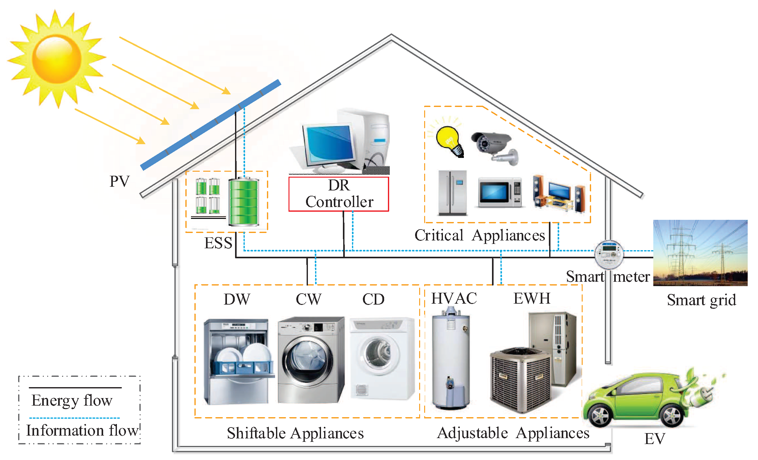
2.1. Models and Constraints of Home Appliances
2.1.1. Adjustable Appliances
2.1.2. Shiftable Appliances
2.1.3. Energy Storage
2.1.4. Electric Vehicle
2.2. DR Optimization Scenarios
2.2.1. Optimal DR for Adjustable Appliances
2.2.2. Optimal DR Policy Considering Shiftable Appliances
2.2.3. Optimal DR Policy Combining ESS and PV
2.2.4. Integrative Optimal DR Policy
3. Approximate Dynamic Programming
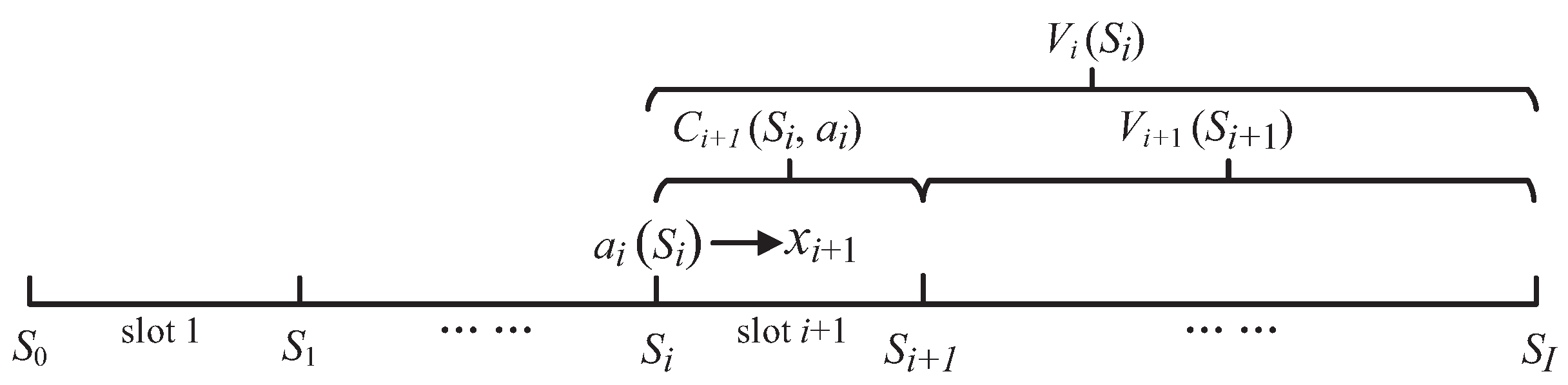
3.1. Problem Reformulation
3.2. ADP for the Integrative DR
3.3. Approximating Functions’ Design
| Algorithm 1. AOPI. |
| Input: |
| 1. Approximate function ; |
| 2. Initial policy ; |
| 3. ; |
| Output: Optimal parameter vector for all i; optimal decision policy ; |
| 4. while do |
| 5. Algorithm 2 Policy evaluation; |
| 6. Obtain parameter vector for all i; |
| 7. Solve (31); |
| 8. end while; |
| 9. return for all i. |
| Algorithm 2. Policy evaluation. |
| Input: for all ; |
| Output: for all ; |
| 1. Initialization: ; |
| 2. for do |
| 3. Sample an initial state ; |
| 4. for do |
| 5. Compute ; |
| 6. Compute ; |
| 7. end for |
| 8. for do |
| 9. Compute ; |
| 10. Update by RLS; |
| 11. end for |
| 12. end for; |
| 13. return . |
4. Case Studies
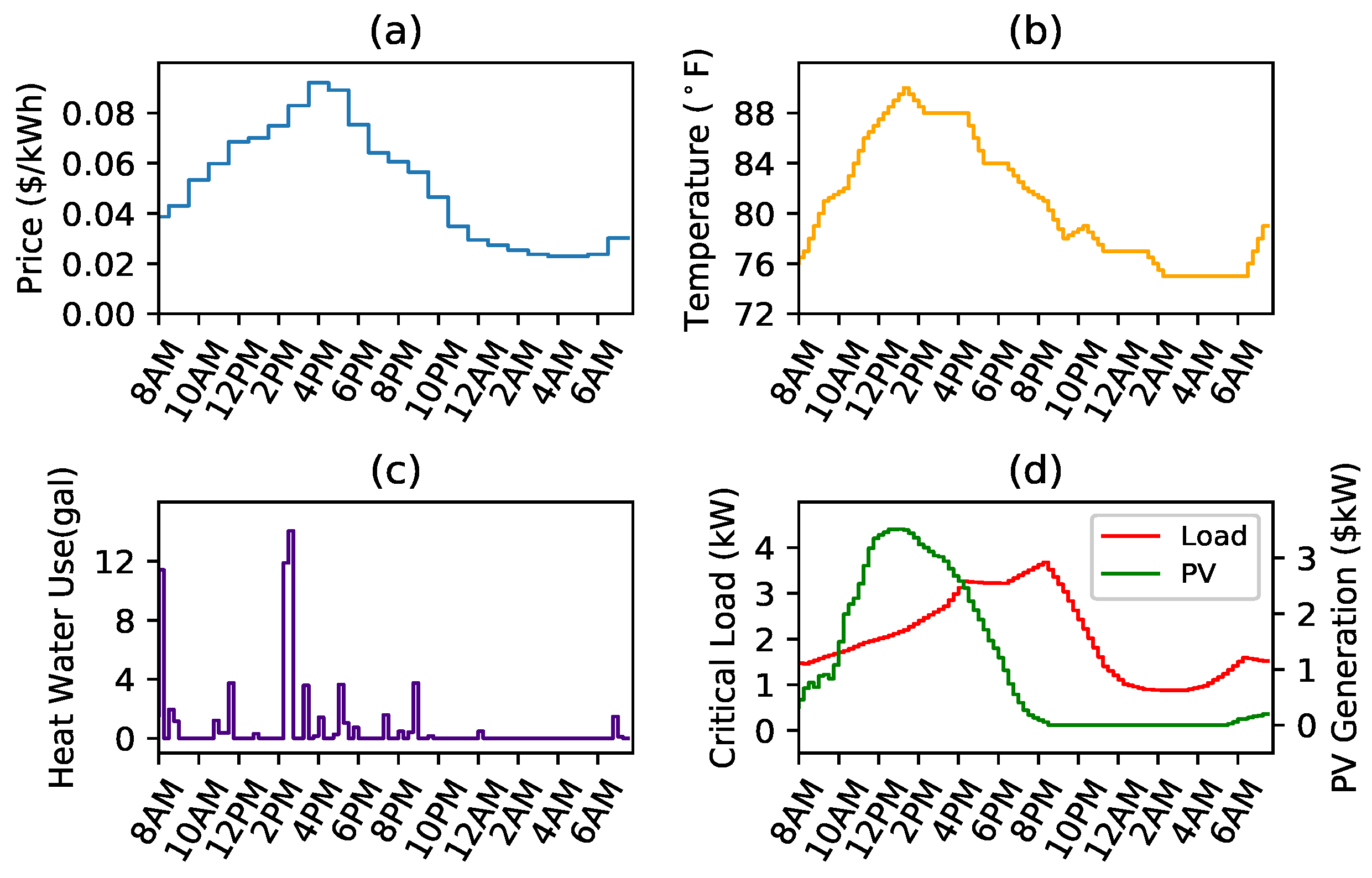
4.1. Parameters
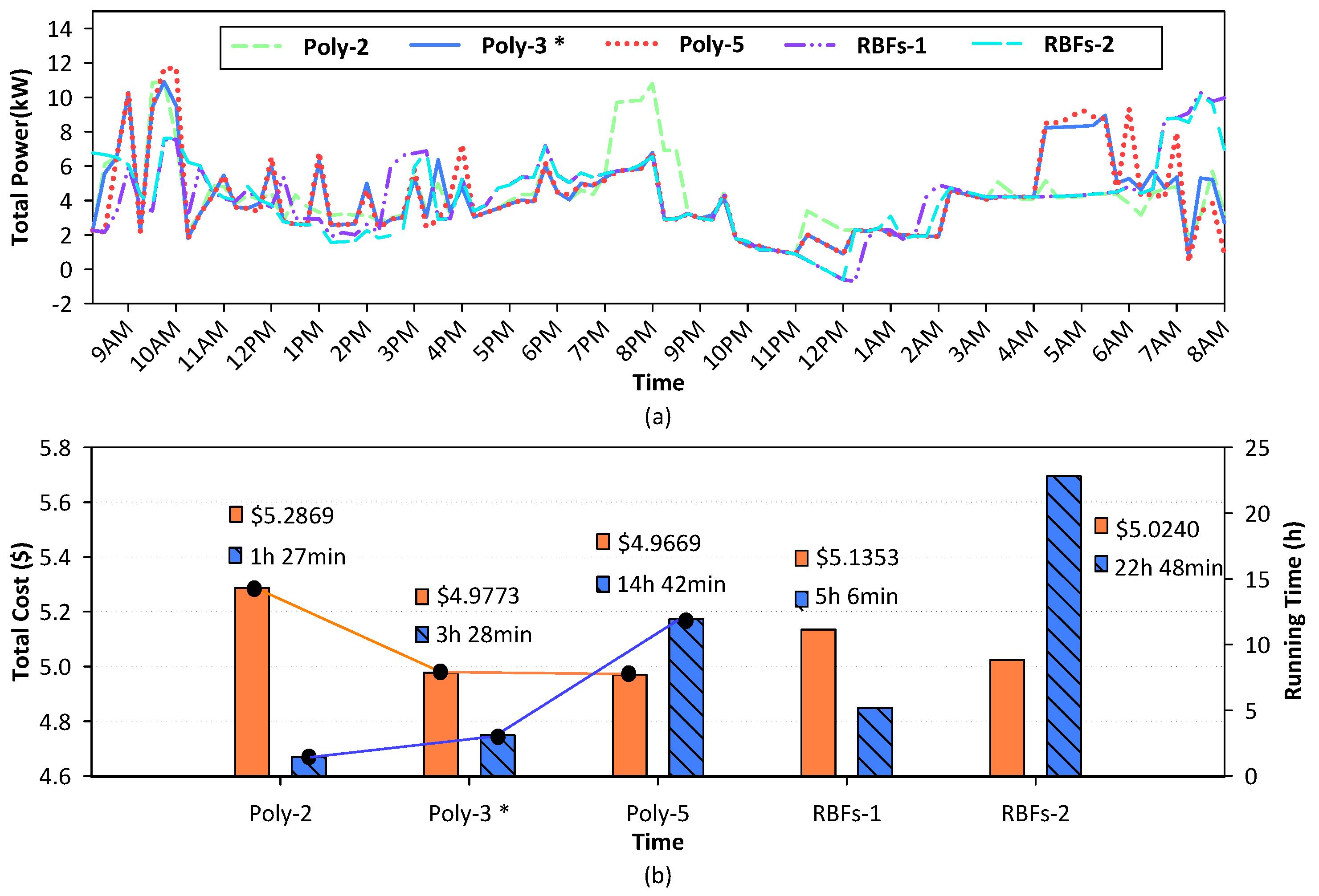
4.2. Different Choices of Approximating Functions
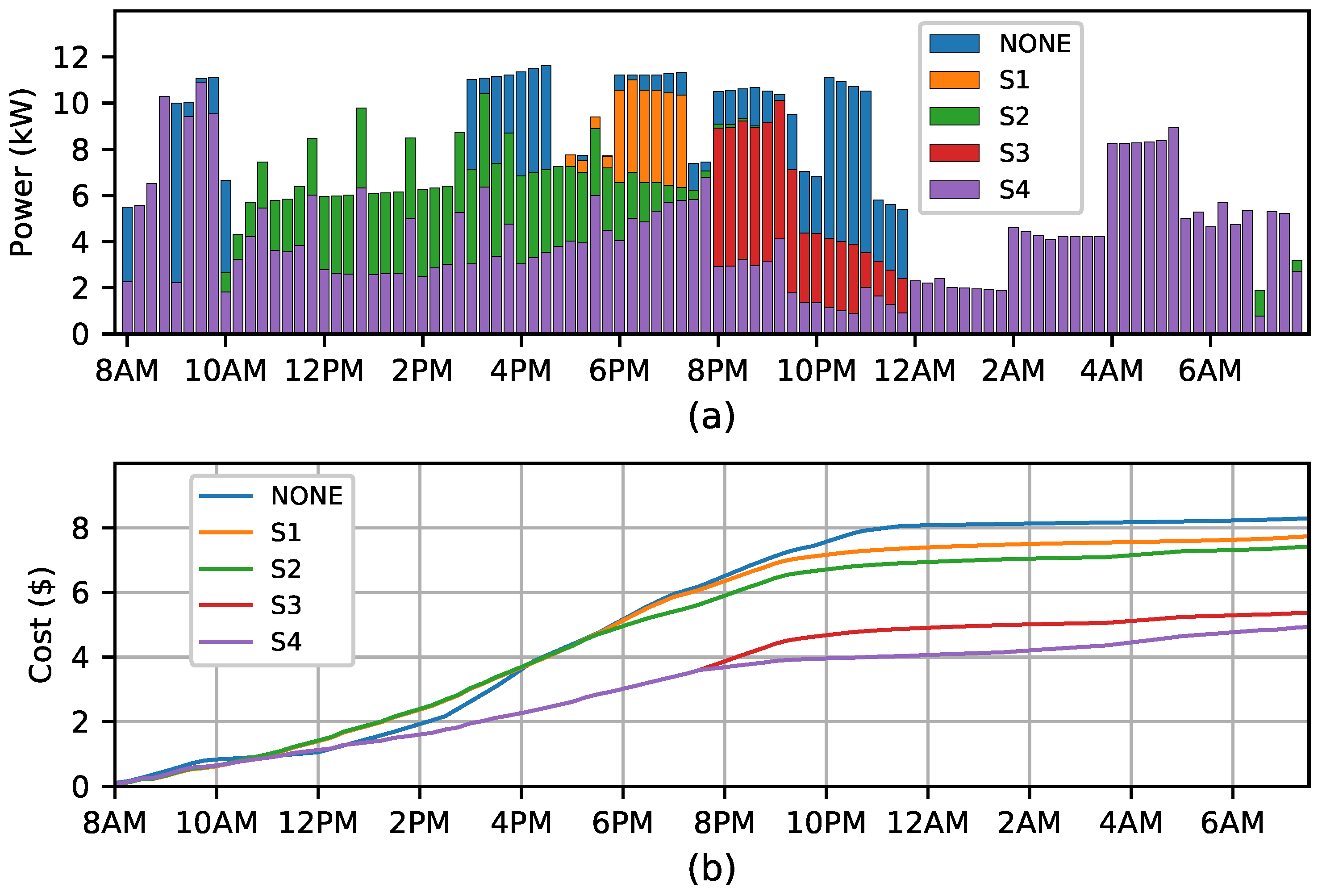
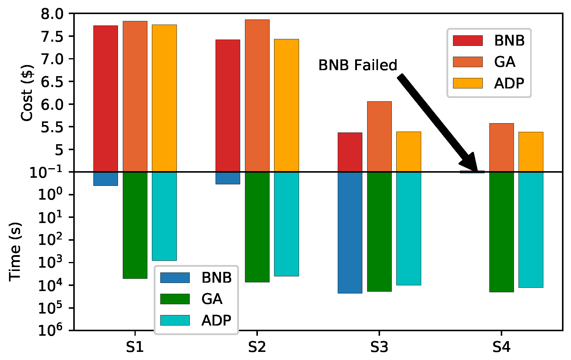
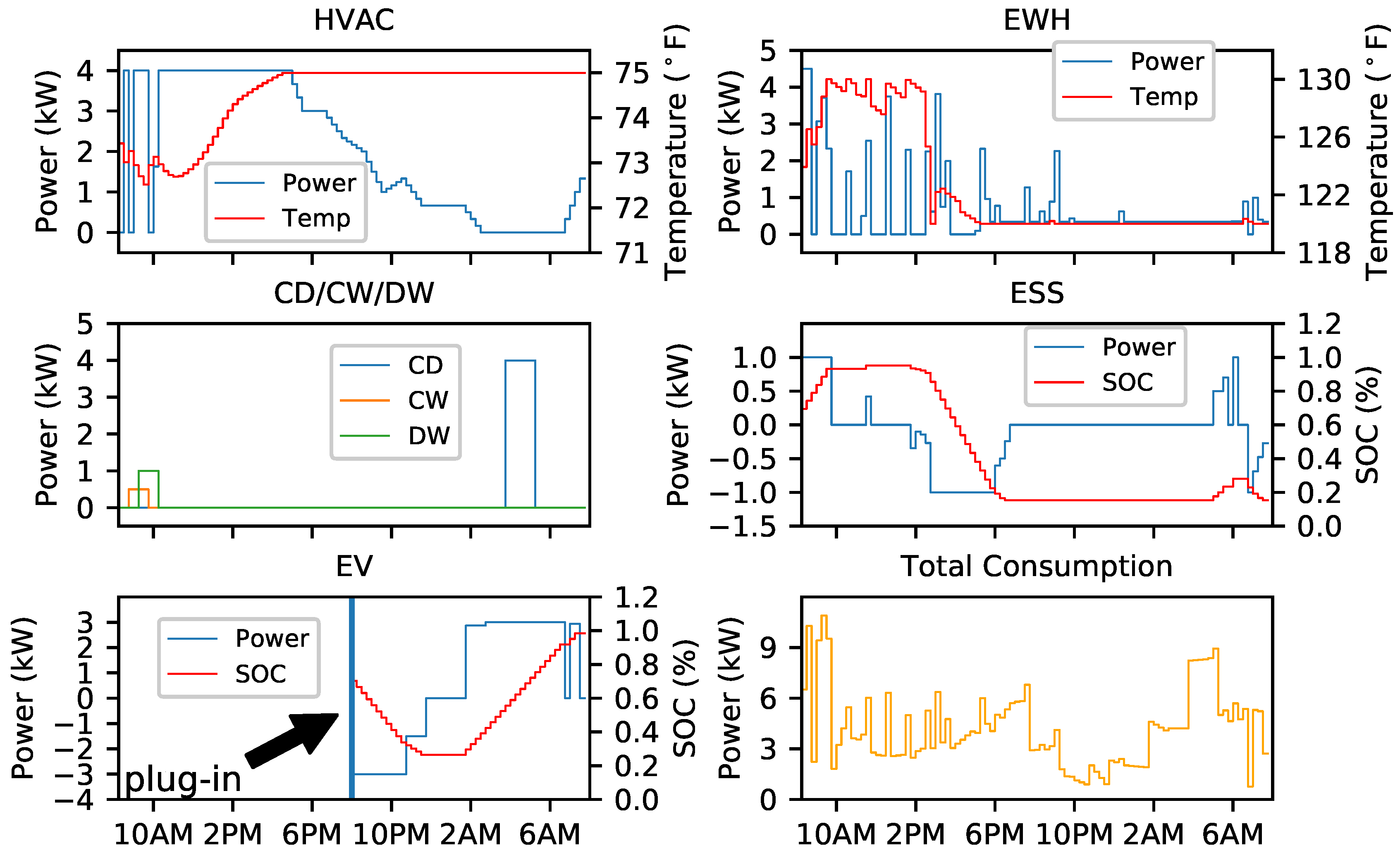
4.3. Comparison of Different Scenarios
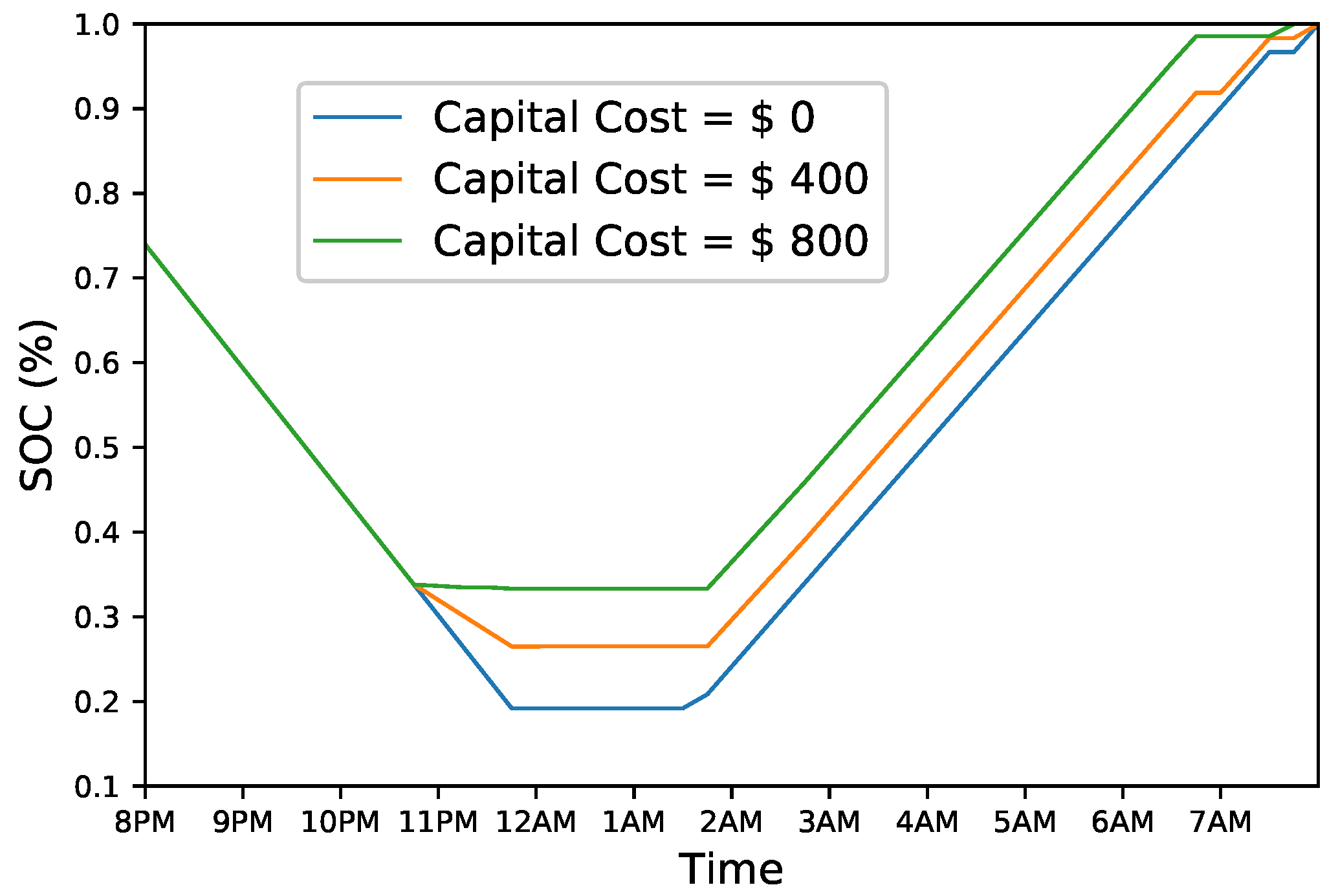
4.4. Discussion and Future Work
5. Conclusions
Acknowledgments
Author Contributions
Conflicts of Interest
Nomenclature
| P | Power (kW) |
| T | Temperature (∘F) |
| E | Energy level of battery (kWh) |
| Battery state of charge (kWh) | |
| Allowable deviation of temperature (∘F) | |
| Efficiency | |
| Inertia factor of air in the house | |
| A | thermal conductivity of the house (kW/∘F) |
| Tank surface area of EWH (ft2) | |
| R | Tank insulation thermal resistance of EWH (hour·ft2·∘F/BTU) |
| Density of water (8.34 lbs/gallon) | |
| F | Hot water flow rate (gallons/hour) |
| Specific heat of water (1.00 BTU/(lbs·∘F)) | |
| Capacity of the EWH tank (gallons) | |
| s | On/off status of a shiftable appliance |
| L | EV battery life |
| Battery depth of discharge | |
| Electricity price ($/kWh) | |
| C | Cost ($) |
| V | Value function |
| S | State vector |
| a | Action vector |
| Set of all feasible actions | |
| DR control policy | |
| Regression parameters of the value function approximator | |
| Duration of a time slot | |
| Superscripts: | |
| Heating, ventilation and air conditioning | |
| Electric water heater | |
| Cloth washer | |
| Cloth dryer | |
| Dish washer | |
| Energy storage system | |
| Electric vehicle | |
| Photovoltaics | |
| Adjustable appliances | |
| Shiftable appliances | |
| Critical appliances | |
| Index of iteration for approximate optimistic policy iteration (AOPI) algorithm | |
| Index of iteration for policy evaluation in the n-th iteration of AOPI | |
| * | Optimum |
| Subscripts: | |
| i | Index of time slot |
| Indoor | |
| Outdoor | |
| Setting value by users | |
| Maximum value | |
| Minimum value | |
| Cold water | |
| Charging | |
| Discharging | |
| Degradation of the battery |
References
- Deng, R.; Yang, Z.; Chow, M.Y.; Chen, J. A survey on demand response in smart grids: Mathematical models and approaches. IEEE Trans. Ind. Inform. 2015, 11, 570–582. [Google Scholar] [CrossRef]
- Association of Home Appliance Manufactures (AHAM). Smart Grid White Paper: The Home Appliance Industrys Principles & Requirements for Achieving a Widely Accepted Smart Grid. Available online: https://www.smartgrid.gov/document/smart_grid (accessed on 20 May 2015).
- Zhao, Z.; Lee, W.C.; Shin, Y.; Song, K.-B. An optimal power scheduling method for demand response in home energy management system. IEEE Trans. Smart Grid 2013, 4, 1391–1400. [Google Scholar] [CrossRef]
- Vardakas, J.; Zorba, N.; Verikoukis, C. A survey on demand response programs in smart grids: Pricing methods and optimization algorithms. IEEE Commun. Surv. Tutor. 2015, 17, 152–178. [Google Scholar] [CrossRef]
- Zhang, D.; Li, S.; Sun, M.; O’Neill, Z. An Optimal and Learning–Based Demand Response and Home Energy Management System. IEEE Trans. Smart Grid 2016, 7, 1790–1801. [Google Scholar] [CrossRef]
- Erdinc, O.; Tascikaraoglu, A.; Paterakis, N.G.; Eren, Y.; Catalao, J.P.S. End-User Comfort Oriented Day-Ahead Planning for Responsive Residential HVAC Demand Aggregation Considering Weather Forecasts. IEEE Trans. Smart Grid 2017, 8, 362–372. [Google Scholar] [CrossRef]
- Pourmousavi, S.A.; Patrick, S.N.; Nehrir, M.H. Real-Time Demand Response Through Aggregate Electric Water Heaters for Load Shifting and Balancing Wind Generation. IEEE Trans. Smart Grid 2014, 5, 769–778. [Google Scholar] [CrossRef]
- Wei, Q.; Liu, D.; Shi, G.; Liu, Y. Multibattery Optimal Coordination Control for Home Energy Management Systems via Distributed Iterative Adaptive Dynamic Programming. IEEE Trans. Smart Grid 2015, 7, 4203–4214. [Google Scholar] [CrossRef]
- Althaher, S.; Mancarella, P.; Mutale, J. Automated Demand Response From Home Energy Management System Under Dynamic Pricing and Power and Comfort Constraints. IEEE Trans. Smart Grid 2015, 6, 1874–1883. [Google Scholar] [CrossRef]
- Anvari-Moghaddam, A.; Monsef, H.; Rahimi-Kian, A. Optimal Smart Home Energy Management Considering Energy Saving and a Comfortable Lifestyle. IEEE Trans. Smart Grid 2015, 6, 324–332. [Google Scholar] [CrossRef]
- Roh, H.T.; Lee, J.W. Residential Demand Response Scheduling With Multiclass Appliances in the Smart Grid. IEEE Trans. Smart Grid 2016, 7, 94–104. [Google Scholar] [CrossRef]
- Muratori, M.; Rizzoni, G. Residential Demand Response: Dynamic Energy Management and Time-Varying Electricity Pricing. IEEE Trans. Power Syst. 2016, 31, 1108–1117. [Google Scholar] [CrossRef]
- Erdinc, O.; Paterakis, N.G.; Mendes, T.D.P.; Bakirtzis, A.G.; Catalão, J.P.S. Smart Household Operation Considering Bi-Directional EV and ESS Utilization by Real-Time Pricing-Based DR. IEEE Trans. Smart Grid 2015, 6, 1281–1291. [Google Scholar] [CrossRef]
- Rastegar, M.; Fotuhi-Firuzabad, M. Outage Management in Residential Demand Response Programs. IEEE Trans. Smart Grid 2015, 6, 1453–1462. [Google Scholar] [CrossRef]
- Paterakis, N.G.; Erdinc, O.; Bakirtzis, A.G.; Catalão, J.P.S. Optimal Household Appliances Scheduling Under Day-Ahead Pricing and Load-Shaping Demand Response Strategies. IEEE Trans. Ind. Inform. 2015, 6, 1509–1519. [Google Scholar] [CrossRef]
- U.S. Department of Commerce. Electricity Storage in Buildings for Residential Sector Demand Response: Control Algorithms and Economic Viability Evaluation. Available online: http://dx.doi.org/10.6028/NIST.GCR.14-978 (accessed on 15 April 2016).
- Farzin, H.; Fotuhi-Firuzabad, M.; Moeini-Aghtaie, M. A Practical Scheme to Involve Degradation Cost of Lithium–Ion Batteries in Vehicle-to-Grid Applications. IEEE Trans. Sustain. Energy 2016, 7, 1730–1738. [Google Scholar] [CrossRef]
- Erdinc, O. Economic impacts of small-scale own generating and storage units, and electric vehicles under different demand response strategies for smart households. Appl. Energy 2014, 126, 142–150. [Google Scholar] [CrossRef]
- Mohsenian-Rad, A.H.; Wong, V.W.S.; Jatskevich, J.; Schober, R.; Leon-Garcia, A. Autonomous Demand-Side Management Based on Game-Theoretic Energy Consumption Scheduling for the Future Smart Grid. IEEE Trans. Smart Grid 2010, 1, 320–331. [Google Scholar] [CrossRef]
- Powell, W.B. Approximate Dynamic Programming, 2nd ed.; David, N.A.C., Balding, J., Eds.; Publishing House: Westfield, NJ, USA, 2011. [Google Scholar]
- Samadi, P.; Mohsenian-Rad, H.; Wong, V.; Schober, R. Real-time pricing for demand response based on stochastic approximation. IEEE Trans. Smart Grid 2014, 5, 789–798. [Google Scholar] [CrossRef]
- Simao, H.; Jeong, H.; Defourny, B.; Powell, W.; Boulanger, A.; Gagneja, A.; Wu, L.; Anderson, R. A robust solution to the load curtailment problem. IEEE Trans. Smart Grid 2013, 4, 2209–2219. [Google Scholar] [CrossRef]
- Wei, Q.; Liu, D.; Shi, G. A novel dual iterative Q-learning method for optimal battery management in smart residential environments. IEEE Trans. Ind. Electron. 2015, 62, 2509–2518. [Google Scholar] [CrossRef]
- Fuselli, D.; Angelis, F.D.; Boaro, M.; Squartini, S.; Wei, Q.; Liu, D.; Piazza, F. Action dependent heuristic dynamic programming for home energy resource scheduling. Int. J. Electr. Power Energy Syst. 2013, 48, 148–160. [Google Scholar] [CrossRef]
- Black, J.W. Integrating Demand into the U.S. Electric Power System: Technical, Economic, and Regulatory Frameworks for Responsive Load. Ph.D. Thesis, Massachusetts Institute of Technology, Cambridge, MA, USA, 2005. Available online: http://hdl.handle.net/1721.1/31168 (accessed on 5 August 2015).
- Nehrir, M.; Jia, R.; Pierre, D.; Hammerstrom, D. Power management of aggregate electric water heater loads by voltage control. In Proceedings of the 2007 IEEE Power Engineering Society General Meeting, Tampa, FL, USA, 24–28 June 2007; pp. 1–6. [Google Scholar]
- Zhou, C.; Qian, K.; Allan, M.; Zhou, W. Modeling of the cost of ev battery wear due to v2g application in power systems. IEEE Trans. Energy Convers. 2011, 26, 1041–1050. [Google Scholar] [CrossRef]
- Bellman, R. Dynamic Programming, 6th ed.; David, N.A.C., Balding, J., Eds.; Princeton University: Princeton, NJ, USA, 1957. [Google Scholar]
- Davis, P.J. Interpolation and Approximation, 1st ed.; ser. Dover Books on Mathematics; Dover: New York, NY, USA, 2014. [Google Scholar]
- Bertsekas, D.P.; Tsitsiklis, J.N. Neuro-Dynamic Programming, 1st ed.; Athena Scientific: Belmont, MA, USA, 1996. [Google Scholar]
- Champaign-Urbana. Department of Atmospheric Sciences, University of Illinois. Available online: https://www.atmos.illinois.edu/weather/daily/index.html (accessed on 10 July 2016).
- Iea/ecbcs Annex 42. Available online: http://www.ieaannex54.org/annex42/index.html (accessed on 10 July 2016).
- EERE. Commercial and Residential Hourly Load Profiles for All tmy3 Locations in The United States. Available online: http://en.openei.org/datasets/?les/961/pub/ (accessed on 10 July 2016).
- Ameren Illinois. Available online: http://www.ameren.com/account/retail-energy (accessed on 10 July 2016).
- Yalmip. Available online: http://users.isy.liu.se/johanl/yalmip/pmwiki.php?n=Main.HomePage (accessed on 11 July 2017 ).
- Yu, M.; Hong, S.H. A Real-Time Demand-Response Algorithm for Smart Grids: A Stackelberg Game Approach. IEEE Trans. Smart Grid 2016, 7, 879–888. [Google Scholar] [CrossRef]
- Forouzandehmehr, N.; Esmalifalak, M.; Mohsenian–Rad, H.; Han, Z. Autonomous Demand Response Using Stochastic Differential Games. IEEE Trans. Smart Grid 2015, 6, 291–300. [Google Scholar] [CrossRef]
- Tran, N.H.; Tran, D.H.; Ren, S.; Han, Z.; Huh, E.N.; Hong, C.S. How Geo-Distributed Data Centers Do Demand Response: A Game-Theoretic Approach. IEEE Trans. Smart Grid 2016, 7, 937–947. [Google Scholar] [CrossRef]
- Maharjan, S.; Zhu, Q.; Zhang, Y.; Gjessing, S.; Basar, T. Dependable Demand Response Management in the Smart Grid: A Stackelberg Game Approach. IEEE Trans. Smart Grid 2013, 7, 120–132. [Google Scholar] [CrossRef]
- Chai, B.; Chen, J.; Yang, Z.; Zhang, Y. Demand Response Management With Multiple Utility Companies: A Two-Level Game Approach. IEEE Trans. Smart Grid 2014, 5, 722–731. [Google Scholar] [CrossRef]


| HVAC | |||||||
|---|---|---|---|---|---|---|---|
| A | |||||||
| 73 ∘F | 2 ∘F | 73 ∘F | 4 kW | 0.95 | 3 | 0.25 | |
| EWH | |||||||
| A | |||||||
| 125 ∘F | 5 ∘F | 125 ∘F | 60 ∘F | 4.5 kW | 24.1 ft2 | 15 | 40 gal |
| ESS | |||||||
| 5 kWh | 0.6 | 1 | 0.2 | 1 kW/1kW | 0.95/0.95 | ||
| EV | |||||||
| 21.6 kWh | 1 | 0.15 | 3 kW | 3 kW | |||
| 0.95 | [46,96] | 211.9$/kWh | 5.6 miles/kWh | 25.68 miles | |||
| CW/DW/CD | |||||||
| 9:00 a.m.–6:00 p.m. | |||||||
| 9:30 a.m.–5:00 p.m. | |||||||
| 6:00 p.m.–8:00 p.m. | |||||||
| P1 | P2 | P3 | P4 | |||||
|---|---|---|---|---|---|---|---|---|
| cost ($) | time (s) | cost ($) | time (s) | cost ($) | time (s) | cost ($) | time (s) | |
| BNB | 7.7333 | 0.4 | 7.4176 | 0.4 | 5.3708 | 22734 | - | - |
| 1-9 GA * | 7.8293 | 5109 | 7.8633 | 7431 | 6.0596 | 19,104 | 5.5741 | 20,174 |
| ADP | 7.7497 | 808 | 7.4304 | 4032 | 5.3807 | 10,142 | 4.9773 | 12,481 |
© 2017 by the authors. Licensee MDPI, Basel, Switzerland. This article is an open access article distributed under the terms and conditions of the Creative Commons Attribution (CC BY) license (http://creativecommons.org/licenses/by/4.0/).
Share and Cite
Li, H.; Zeng, P.; Zang, C.; Yu, H.; Li, S. An Integrative DR Study for Optimal Home Energy Management Based on Approximate Dynamic Programming. Sustainability 2017, 9, 1248. https://doi.org/10.3390/su9071248
Li H, Zeng P, Zang C, Yu H, Li S. An Integrative DR Study for Optimal Home Energy Management Based on Approximate Dynamic Programming. Sustainability. 2017; 9(7):1248. https://doi.org/10.3390/su9071248
Chicago/Turabian StyleLi, Hepeng, Peng Zeng, Chuanzhi Zang, Haibin Yu, and Shuhui Li. 2017. "An Integrative DR Study for Optimal Home Energy Management Based on Approximate Dynamic Programming" Sustainability 9, no. 7: 1248. https://doi.org/10.3390/su9071248
APA StyleLi, H., Zeng, P., Zang, C., Yu, H., & Li, S. (2017). An Integrative DR Study for Optimal Home Energy Management Based on Approximate Dynamic Programming. Sustainability, 9(7), 1248. https://doi.org/10.3390/su9071248