A Hybrid Estimation of Distribution Algorithm for Multi-Objective Multi-Sourcing Intermodal Transportation Network Design Problem Considering Carbon Emissions

Abstract
:1. Introduction
2. Literature Review
3. Problem Description and Model Formulation
3.1. Formulation of Proposed Mathematical Model
| An infinite number; | |
| Amount of freight from sourcing place i, ; | |
| Set of available nodes of stage j, ; | |
| Available nodes of stage 0 and =N; | |
| Available node of stage M and =1; | |
| Set of available transportation modes of stage j, ; | |
| The handling capacity for the kth node of stage j, , , ; | |
| Carbon emission cost of freight i from the lth node in stage to the hth node in stage j under the transportation mode w, , , ; | |
| Transportation cost of freight i from the lth node in stage to the hth node in stage j under the transportation mode w, , , ; | |
| Transportation time of freight i from the lth node in stage to the hth node in stage j under the transportation mode w, , , , ; | |
| Switch cost of freight i from transportation mode w to v for the kth node of stage j, , , , ; | |
| Switch time of freight i from transportation mode w to v for the kth node of stage j, , , , ; and | |
| . | |
| ; |
| ; |
| the start time at the stage j for freight i; and |
| the leave time at the stage j for freight i. |
3.2. Modification of Established Model
4. HEDA for MO_MSITNDP
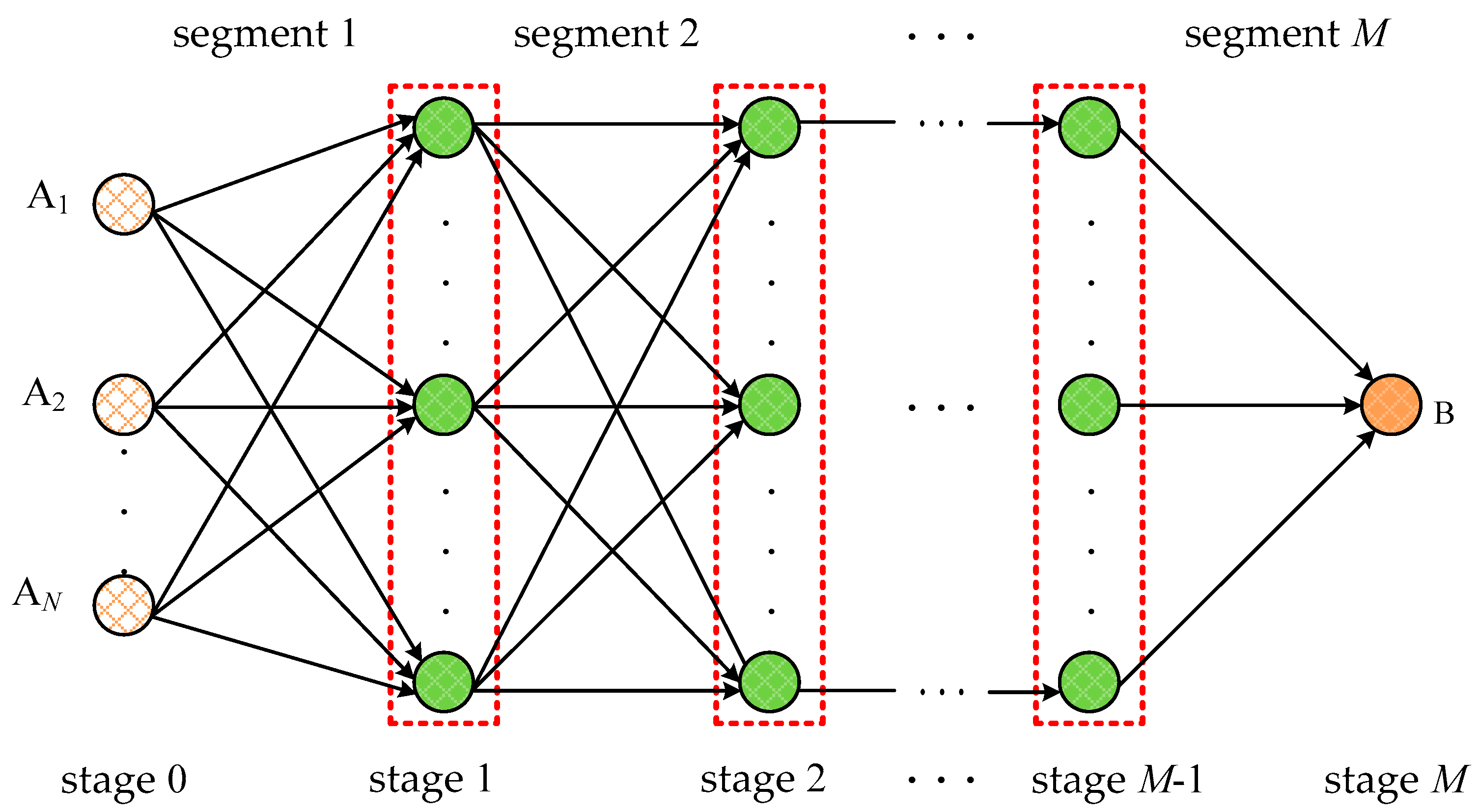
4.1. Solution Representation
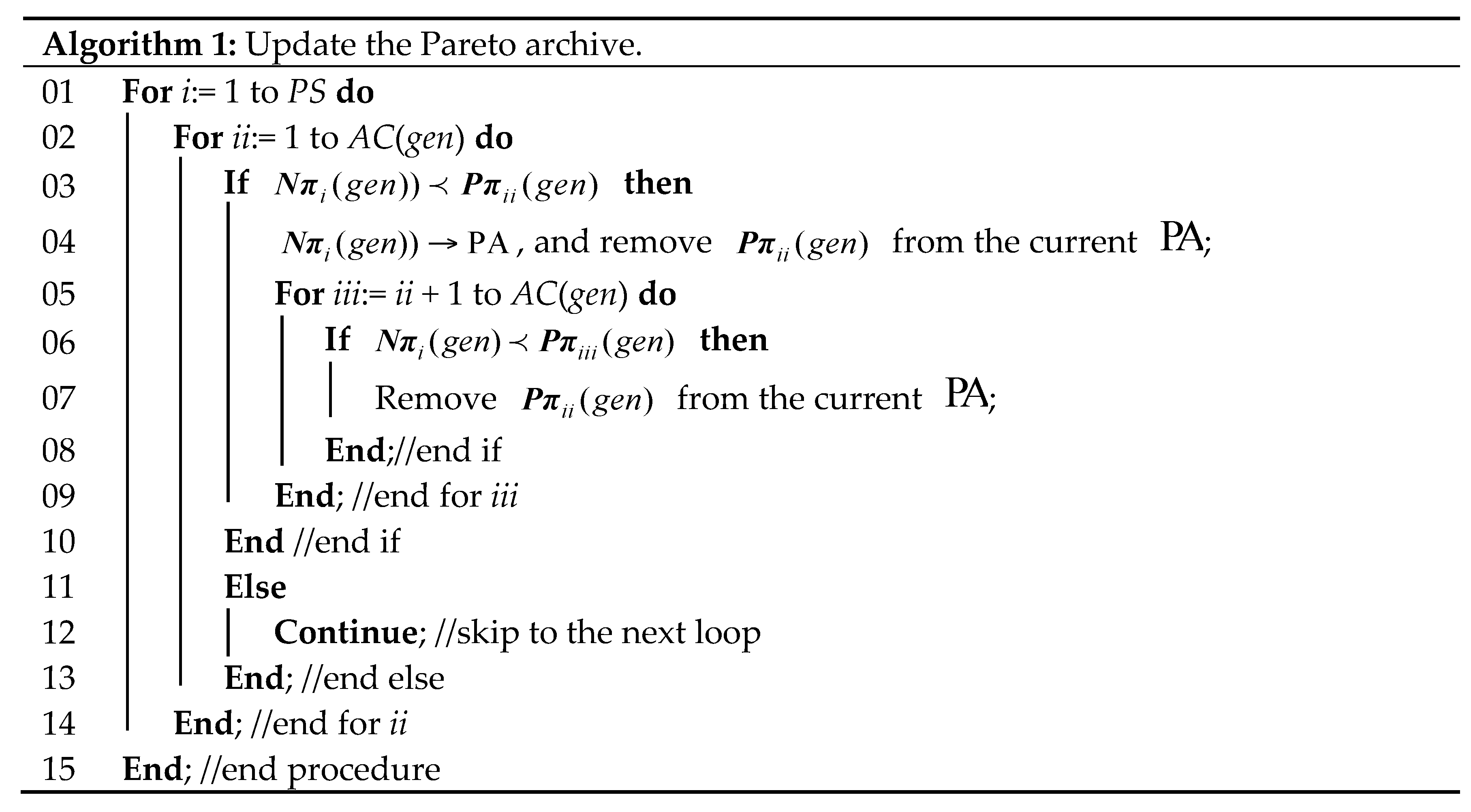
4.2. Multi-Objective Handling Method
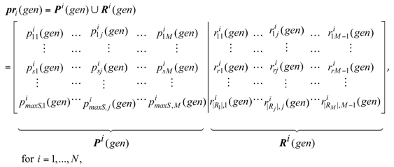
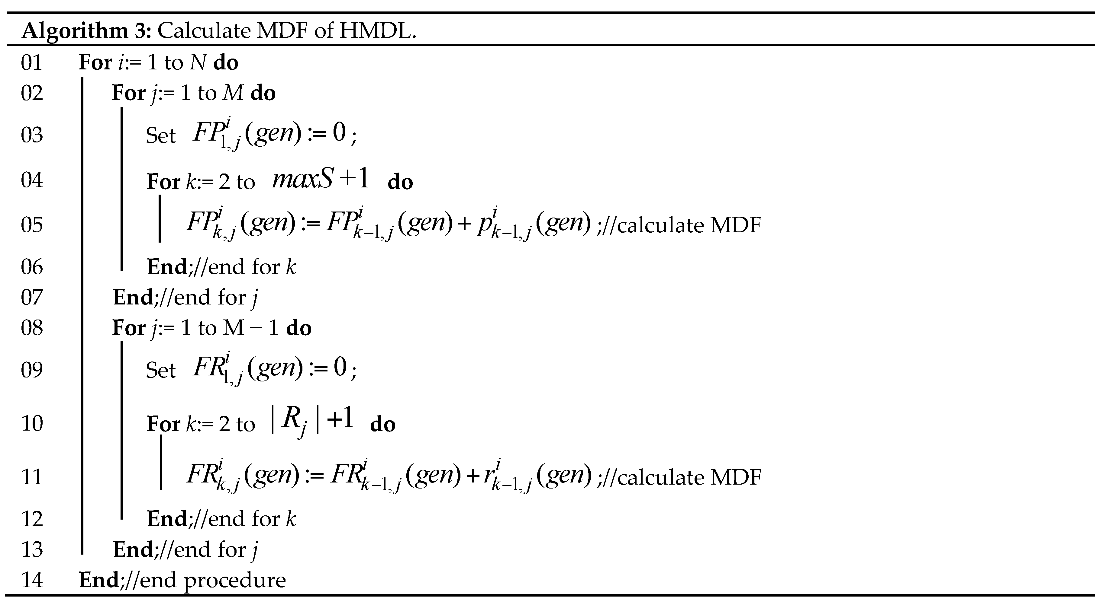
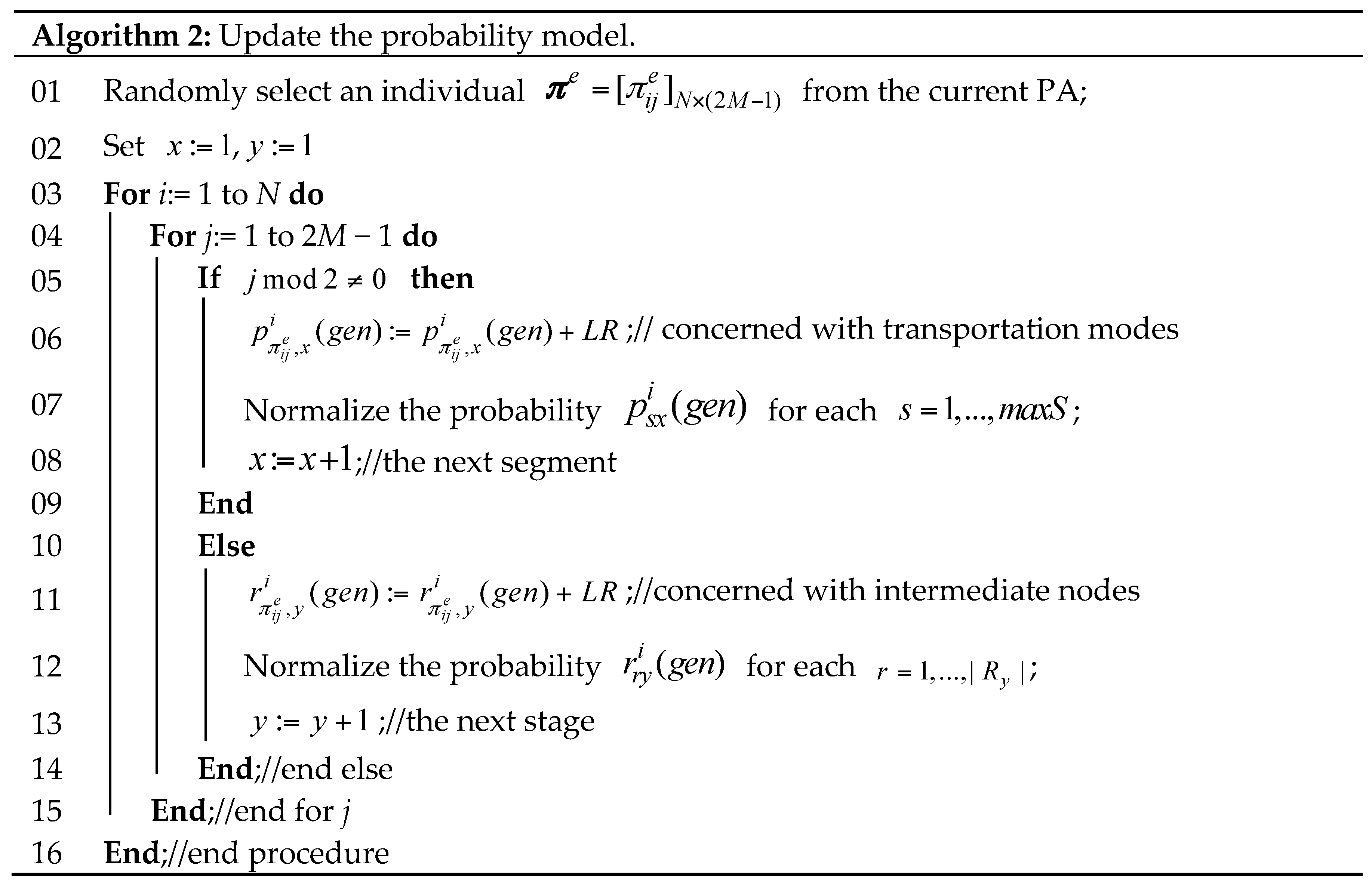
4.3. The Proposed Heterogeneous Probability Model and Update Mechanism
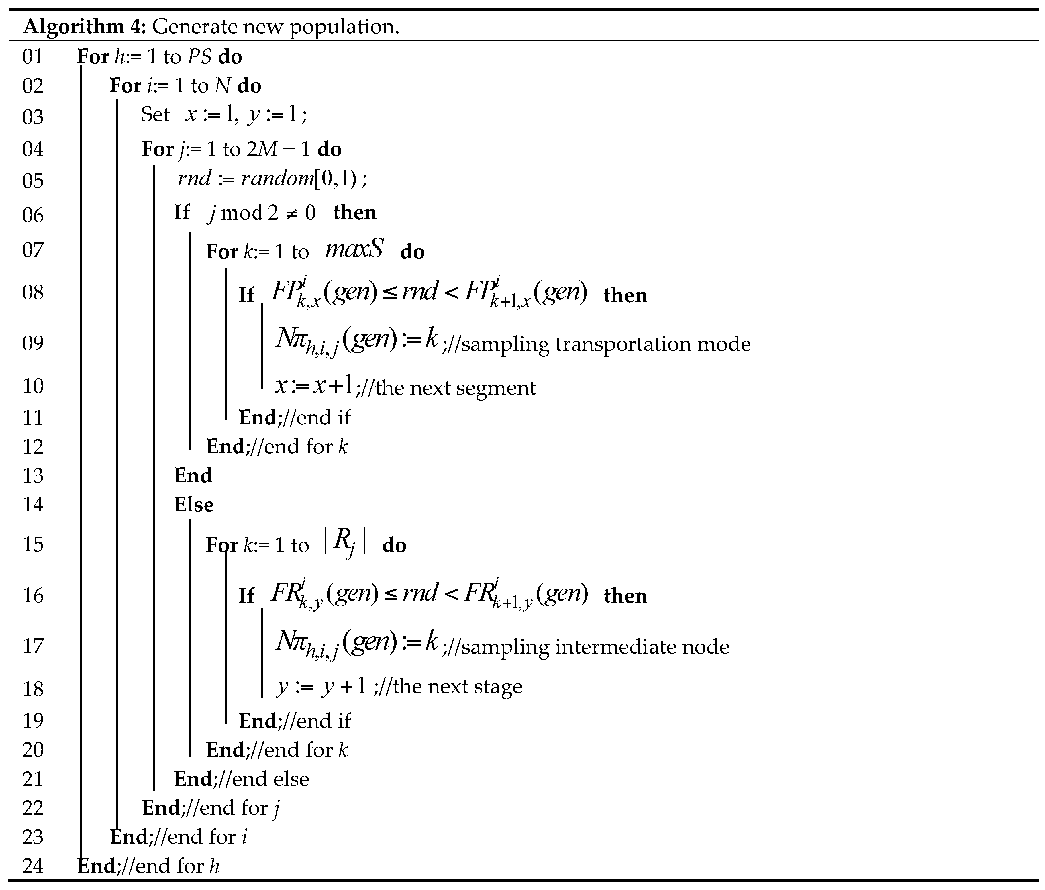
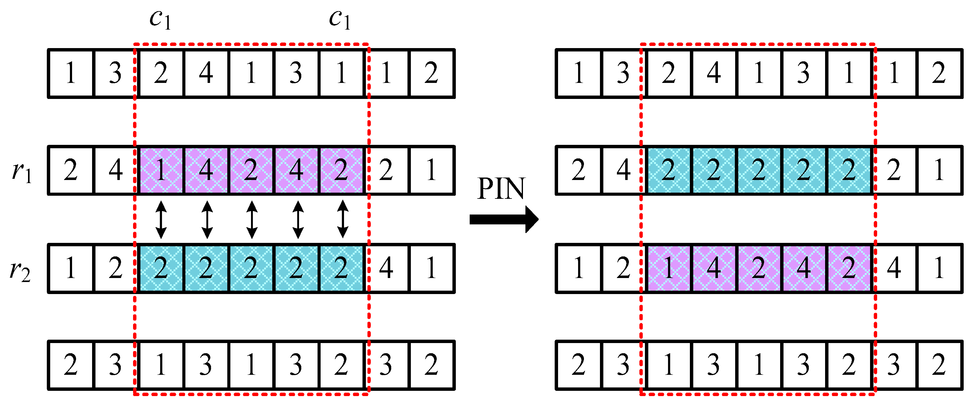
4.4. New Population Generation Method
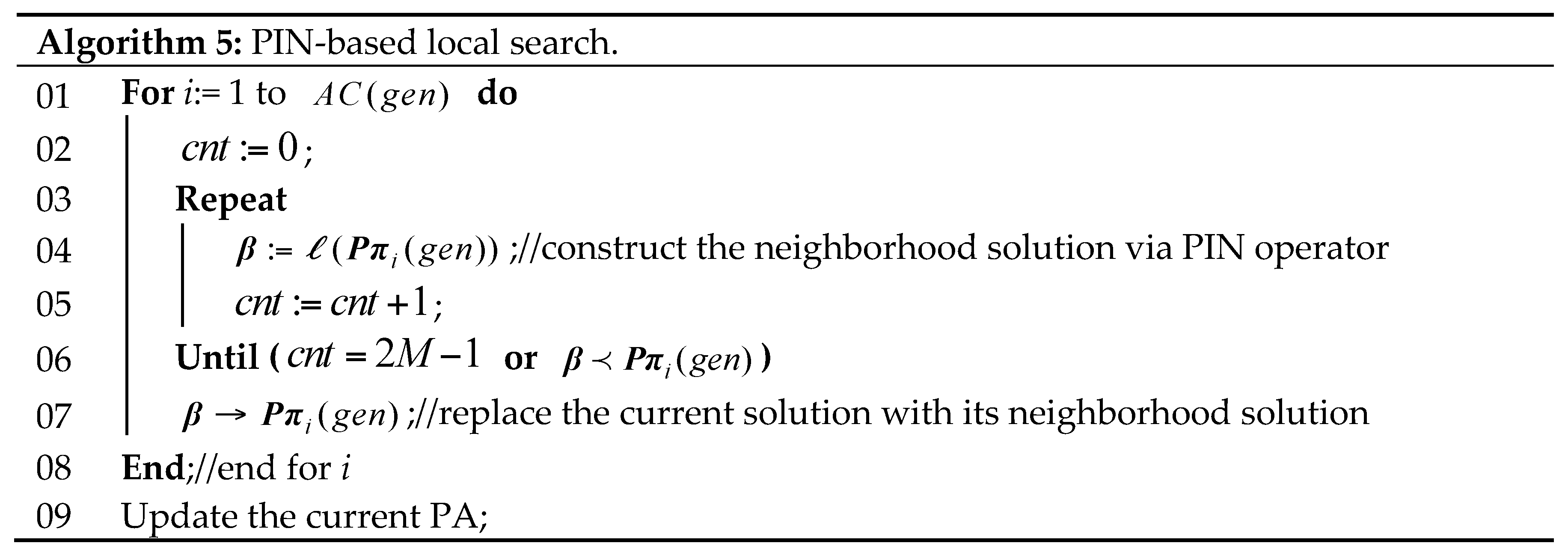
4.5. Problem-Dependent Local Search
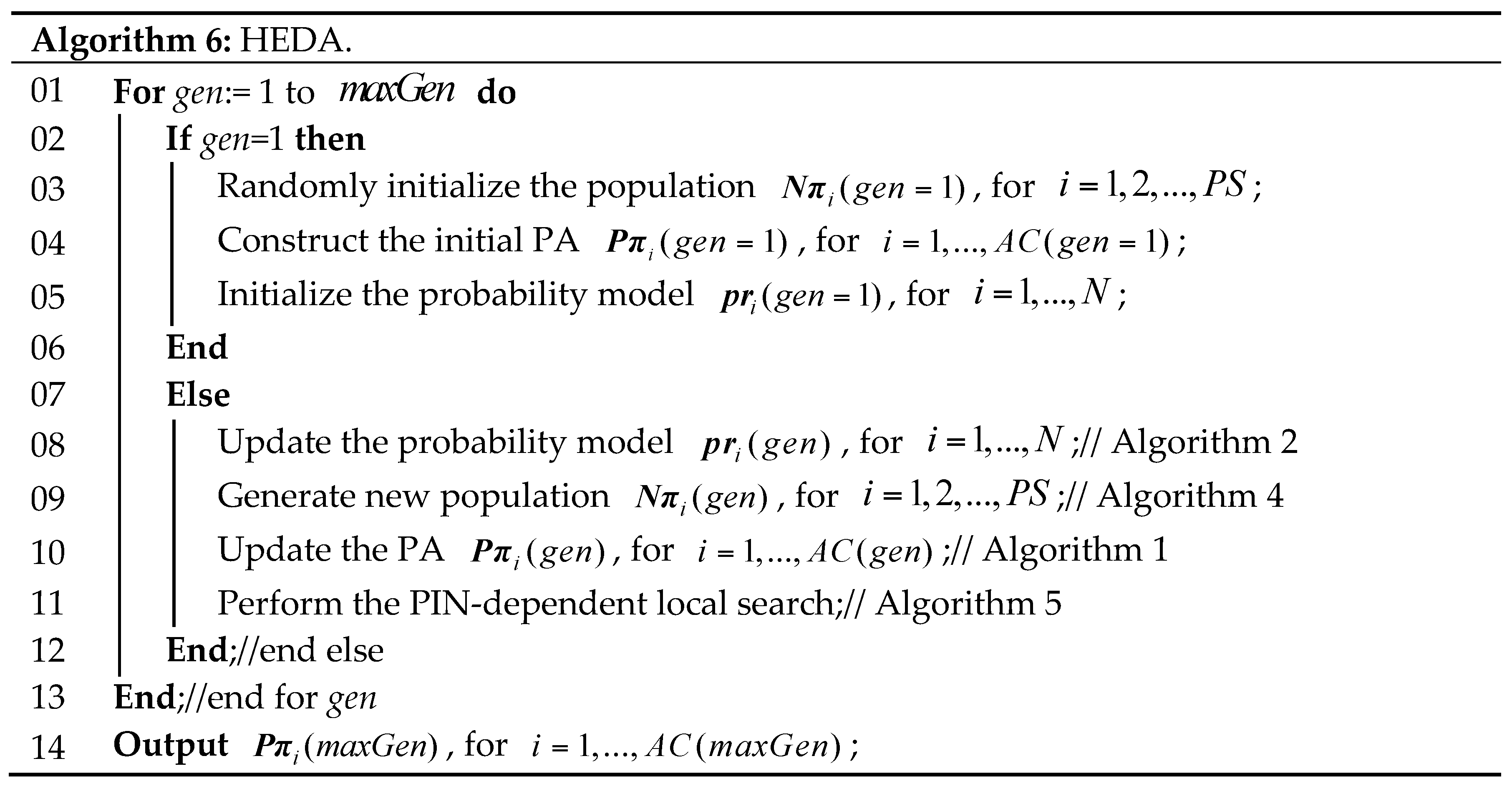
4.6. Procedure of HEDA
5. Computational Results and Comparisons
5.1. Experimental Setup
5.2. Performance Metrics
 is the union of non-dominated solutions with regard to , and then
  is the number of non-dominated solutions in
  which are not dominated by solutions in
  as shown in Equation (20). The larger the value of is, the better performance of Algorithm l.
 , shown as following Equation (21). The higher the value of
  is, the better performance of Algorithm l.
 to [40], then DIR can be defined in Equation (22). Obviously, a smaller
  means a better convergence performance to , as well as a better distribution of .
5.3. Comparisons Results
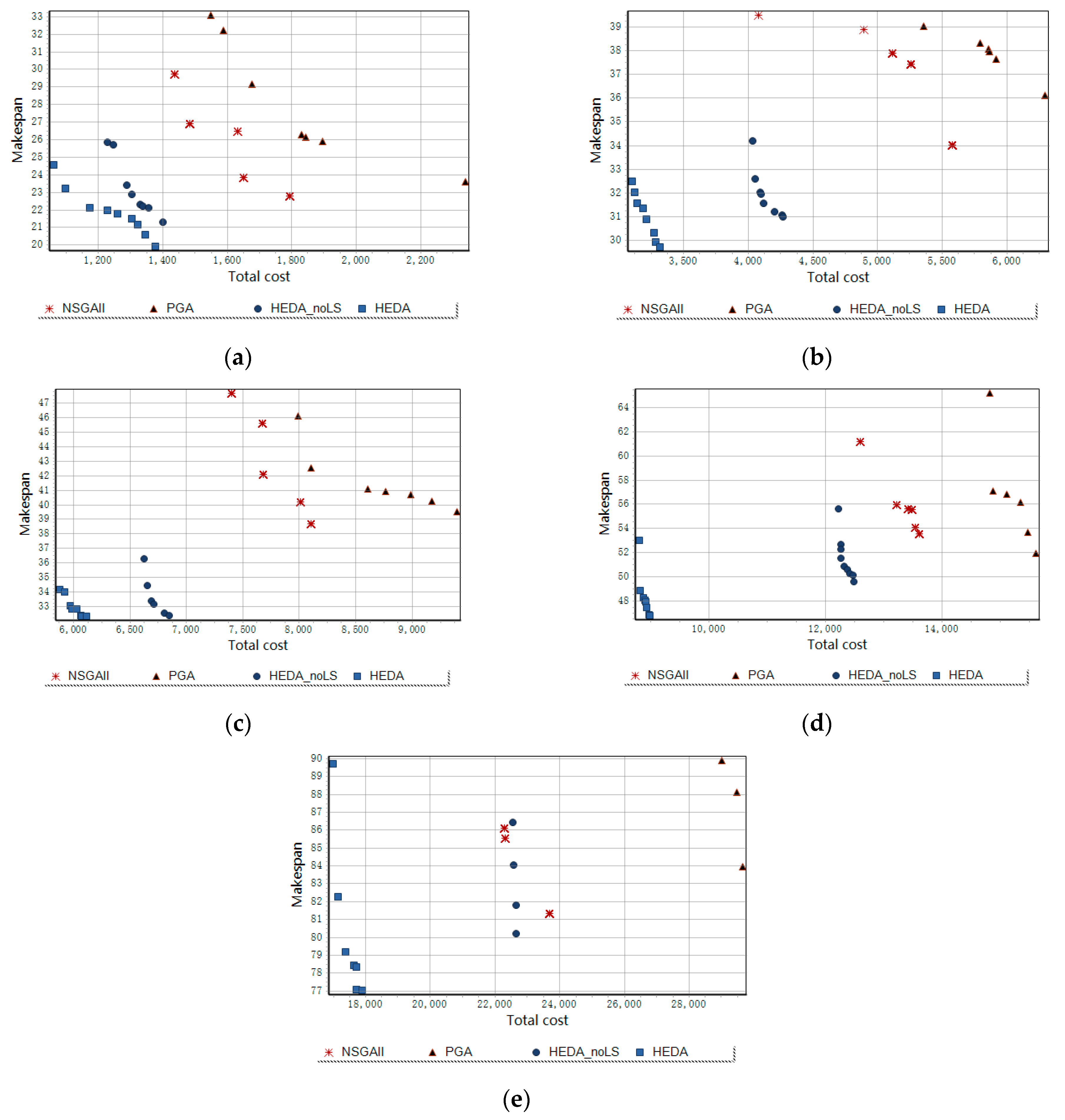
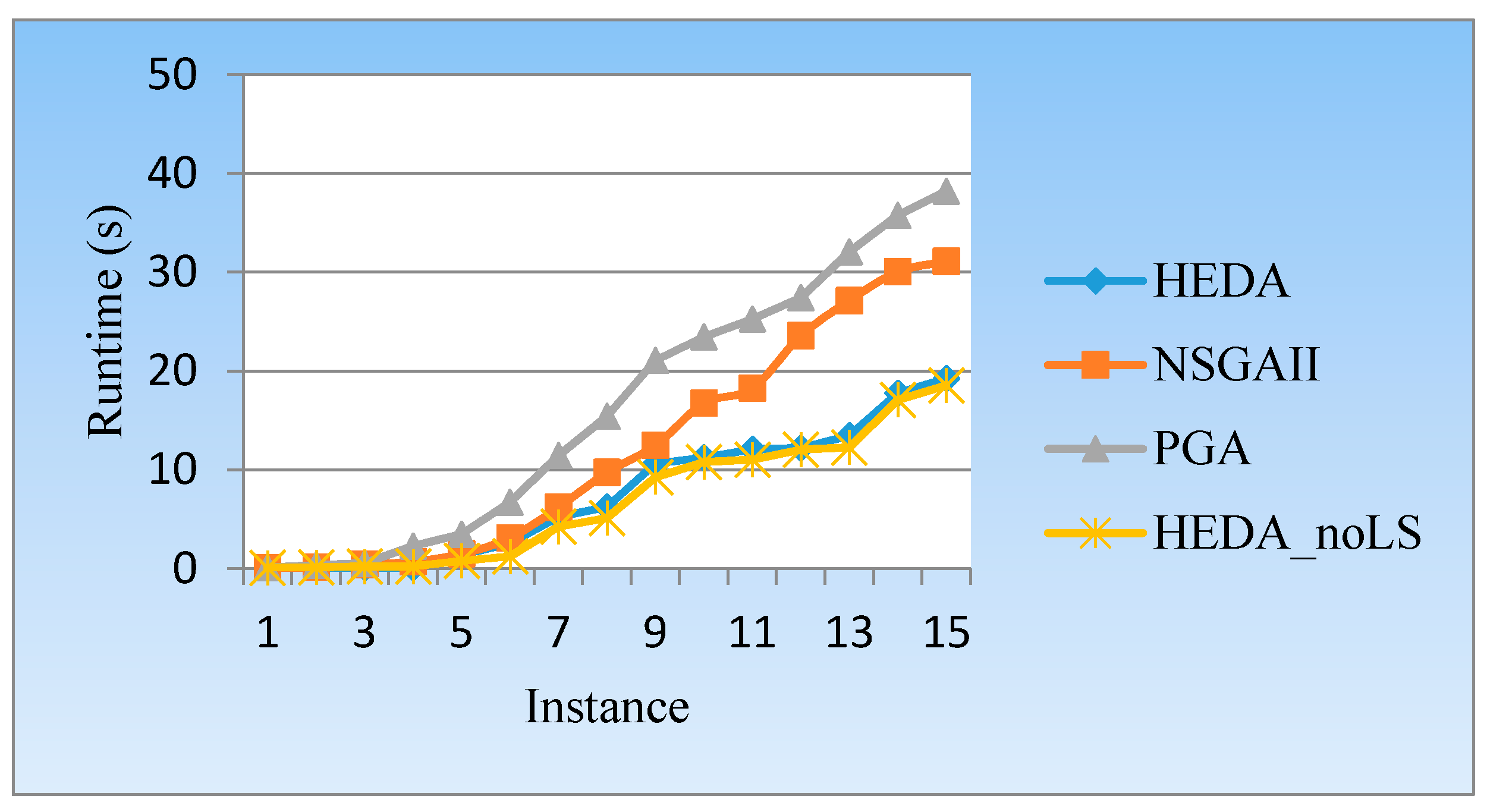
5.3.1. Comparison with Existing Algorithms
5.3.2. Comparison with Optimization Solver
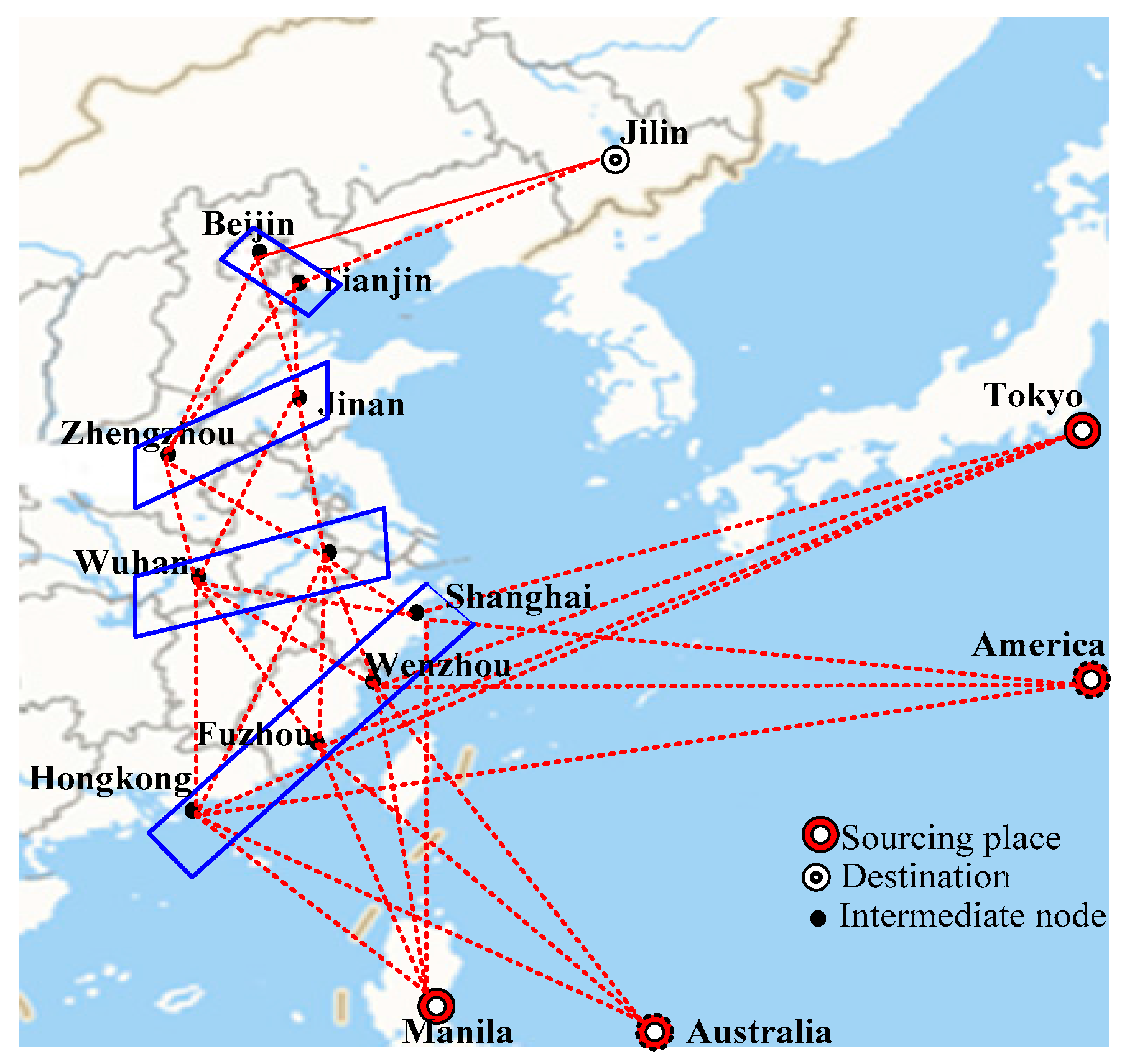
5.4. Case Study
5.5. Management Insights
6. Conclusions
Acknowledgments
Author Contributions
Conflicts of Interest
References
- Duan, X.; Heragu, S. Carbon Emission Tax Policy in an Intermodal Transportation Network. In Proceedings of the IIE Annual Conference, Nashville, TN, USA, 30 May–2 June 2015. [Google Scholar]
- Zheng, H.Y.; Wang, L. Reduction of carbon emissions and project makespan by a Pareto-based estimation of distribution algorithm. Int. J. Prod. Econ. 2015, 164, 421–432. [Google Scholar] [CrossRef]
- Bouchery, Y.; Fransoo, J. Cost, carbon emissions and modal shift in intermodal network design decisions. Int. J. Prod. Econ. 2014, 164, 388–399. [Google Scholar] [CrossRef]
- Li, Y.; Bao, L.; Li, W.; Deng, H. Inventory and Policy Reduction Potential of Greenhouse Gas and Pollutant Emissions of Road Transportation Industry in China. Sustainability 2016, 8, 1218. [Google Scholar] [CrossRef]
- Piecyk, M.I.; Mckinnon, A.C. Forecasting the carbon footprint of road freight transport in 2020. Int. J. Prod. Econ. 2010, 128, 31–42. [Google Scholar] [CrossRef]
- Benjaafar, S.; Li, Y.; Daskin, M. Carbon footprint and the management of supply chains: Insights from simple models. IEEE Trans. Autom. Sci. Eng. 2013, 10, 99–116. [Google Scholar] [CrossRef]
- Lam, S.L.; Gu, Y. A market-oriented approach for intermodal network optimisation meeting cost, time and environmental requirements. Int. J. Prod. Econ. 2016, 171, 266–274. [Google Scholar] [CrossRef]
- Kim, N.S.; Wee, V.B. Toward a better methodology for assessing CO2 emissions for intermodal and truck-only freight systems: A European case study. Int. J. Sustain. Transp. 2014, 8, 177–201. [Google Scholar] [CrossRef]
- Zheng, Y.; Liao, H.; Yang, X. Stochastic Pricing and Order Model with Transportation Mode Selection for Low-Carbon Retailers. Sustainability 2016, 8, 48. [Google Scholar] [CrossRef]
- Craig, A.J.; Blanco, E.E.; Sheffi, Y. Estimating the CO2 intensity of intermodal freight transportation. Transp. Res. D Transp. Environ. 2013, 22, 49–53. [Google Scholar] [CrossRef]
- Kaur, H.; Singh, S.P. Flexible dynamic sustainable procurement model. Ann. Oper. Res. 2017. [Google Scholar] [CrossRef]
- Steadieseifi, M.; Dellaert, N.P.; Nuijten, W.; Woensel, T.V.; Raoufi, R. Multimodal freight transportation planning: A literature review. Eur. J. Oper. Res. 2014, 233, 1–15. [Google Scholar] [CrossRef]
- Meng, Q.; Wang, X. Intermodal hub-and-spoke network design: Incorporating multiple stakeholders and multi-type containers. Transp. Res. B Meth. 2011, 45, 724–742. [Google Scholar] [CrossRef]
- Limbourg, S.; Jourquin, B. Optimal rail-road container terminal locations on the European network. Transp. Res. E Log. 2009, 45, 551–563. [Google Scholar] [CrossRef]
- Vermam, M.; Verter, V.; Zufferey, N. A bi-objective model for planning and managing rail-truck intermodal transportation of hazardous materials. Transp. Res. E Log. 2012, 48, 132–149. [Google Scholar] [CrossRef]
- Francesco, M.D.; Lai, M.; Zuddas, P. Maritime repositioning of empty containers under uncertain port disruptions. Comput. Ind. Eng. 2013, 64, 827–837. [Google Scholar] [CrossRef]
- Bandeira, D.L.; Becker, J.L.; Borenstein, D.A. DSS for integrated distribution of empty and full containers. Decis. Support Syst. 2009, 47, 383–397. [Google Scholar] [CrossRef]
- Yang, X.; Low, J.M.W.; Tang, L.C. Analysis of intermodal freight from China to Indian Ocean: A goal programming approach. J. Transp. Geogr. 2011, 19, 515–527. [Google Scholar] [CrossRef]
- Resat, H.G.; Turkay, M. Design and operation of intermodal transportation network in the Marmara region of Turkey. Transp. Res. E Log. 2015, 83, 16–33. [Google Scholar] [CrossRef]
- Domuţa, C.; Radu, D.; Enache, M.; Aştilean, A. Application for Intermodal Transportation Routing using Bi-objective Time-dependent Modified Algorithm. Acta Electroteh. 2012, 53, 154–159. [Google Scholar]
- Namseok, K.; Janic, M.; Wee, B.V. Trade-off between carbon dioxide emissions and logistics costs based on multi-objective optimization. Transp. Res. Rec. J. Transp. Res. Board 2009, 2139, 107–116. [Google Scholar]
- Rudi, A.; Fröhling, M.; Zimmer, K.; Schultman, F. Freight transportation planning considering carbon emissions and in-transit holding costs: A capacitated multi-commodity network flow model. Eur. J. Transp. Log. 2016, 5, 123–160. [Google Scholar] [CrossRef]
- Demir, E.; Burgholzer, W.; Hrušovský, M.; Arıkan, E.; Jammernegg, W.; Woensel, T.V. A green intermodal service network design problem with travel time uncertainty. Transp. Res. B Meth. 2015, 42, 1439–1443. [Google Scholar] [CrossRef]
- Lee, C.T.; Hashim, H.; Ho, C.S.; Fan, Y.V.; Klemeš, J.J. Sustaining the low-carbon emission development in Asia and beyond: Sustainable energy, water, transportation and low-carbon emission technology. J. Clean. Prod. 2017, 146, 1–13. [Google Scholar] [CrossRef]
- KılıÇ, F.; Gök, M. A demand based route generation algorithm for public transit network design. Comput. Oper. Res. 2014, 51, 21–29. [Google Scholar] [CrossRef]
- Vermam, M.; Verter, V. A lead-time based approach for planning rail–truck intermodal transportation of dangerous goods. Eur. J. Oper. Res. 2010, 202, 696–706. [Google Scholar] [CrossRef]
- An, C.; Macharis, C.; Janssens, G.K. Corridor network design in hinterland transportation systems. Flex. Serv. Manuf. J. 2012, 2, 294–319. [Google Scholar]
- Braekers, K.; An, C.; Janssens, G.K. Optimal shipping routes and vessel size for intermodal barge transport with empty container repositioning. Comput. Ind. 2013, 64, 155–164. [Google Scholar] [CrossRef]
- Ishfaq, R.; Sox, C.R. Design of intermodal logistics networks with hub delays. Eur. J. Oper. Res. 2012, 220, 629–641. [Google Scholar] [CrossRef]
- Li, L.; Negenborn, R.R.; Schutter, B.D. Intermodal freight transport planning—A receding horizon control approach. Transp. Res. C Emerg. 2015, 60, 77–95. [Google Scholar] [CrossRef]
- Sterzik, S.; Kopfer, H.A. Tabu Search Heuristic for the Inland Container Transportation Problem. Comput. Oper. Res. 2013, 40, 953–962. [Google Scholar] [CrossRef]
- Nossack, J.; Pesch, E. A truck scheduling problem arising in intermodal container transportation. Eur. J. Oper. Res. 2013, 230, 666–680. [Google Scholar] [CrossRef]
- Zhang, J.; Zhang, Q.; Zhang, L. A Study on the Paths Choice of Intermodal Transport Based on Reliability, 2014; Springer: Berlin, Germany, 2015; pp. 305–315. [Google Scholar]
- Wang, S.; Wang, L.; Xu, Y.; Liu, M. An effective estimation of distribution algorithm for the flexible job-shop scheduling problem with fuzzy processing time. Int. J. Prod. Res. 2013, 51, 3778–3793. [Google Scholar] [CrossRef]
- Wang, L.; Wang, S.; Zheng, X. A hybrid estimation of distribution algorithm for unrelated parallel machine scheduling with sequence-dependent setup times. IEEE. J. Autom. Sin. 2016, 3, 235–246. [Google Scholar]
- Salcedo-Sanz, S. A survey of repair methods used as constraint handling techniques in evolutionary algorithms. Comput. Sci. Rev. 2009, 3, 175–192. [Google Scholar] [CrossRef]
- Wang, Y.; Cai, Z.; Guo, G.; Zhou, Y.Q. Multiobjective optimization and hybrid evolutionary algorithm to solve constrained optimization problems. IEEE Trans. Syst. Man Cybern. B 2007, 37, 560–575. [Google Scholar] [CrossRef]
- Li, H.; Zhang, Q. Multiobjective optimization problems with complicated Pareto sets, MOEA/D and NSGA-II. IEEE Trans. Evolut. Comput. 2009, 13, 284–302. [Google Scholar] [CrossRef]
- Nowicki, E.; Smutnicki, C. A fast tabu search algorithm for the permutation flow-shop problem. Eur. J. Oper. Res. 1996, 91, 160–175. [Google Scholar] [CrossRef]
- Qian, B.; Wang, L.; Huang, D.X.; Wang, X. Multi-objective no-wait flow-shop scheduling with a memetic algorithm based on differential evolution. Soft Comput. 2009, 13, 847–869. [Google Scholar] [CrossRef]
- Deb, K.; Pratap, A.; Agarwal, S.; Meyarivan, T. A fast and elitist multiobjective genetic algorithm: NSGA-II. IEEE Trans. Evolut. Comput. 2002, 6, 182–197. [Google Scholar] [CrossRef]
- Bérubé, J.F.; Gendreau, M.; Potvin, J.Y. An exact-constraint method for bi-objective combinatorial optimization problems: Application to the traveling salesman problem with profits. Eur. J. Oper. Res. 2009, 194, 39–50. [Google Scholar] [CrossRef]


| Instance | HEDA vs. NSGAII | HEDA vs. PGA | HEDA vs. HEDA_noLS | |||||||||||||||
|---|---|---|---|---|---|---|---|---|---|---|---|---|---|---|---|---|---|---|
| NSGAII | HEDA | PGA | HEDA | HEDA_noLS | HEDA | |||||||||||||
| MAX | AVG | SD | MAX | AVG | SD | MAX | AVG | SD | MAX | AVG | SD | MAX | AVG | SD | MAX | AVG | SD | |
| 44 | 20.24 | 14.45 | 5 | 3.71 | 0.63 | 3 | 1.57 | 0.79 | 5 | 3.81 | 0.59 | 4 | 2.52 | 1.26 | 4 | 2.81 | 0.96 | |
| 53 | 6.29 | 13.99 | 8 | 5.48 | 1.65 | 2 | 0.10 | 0.43 | 6 | 4.57 | 1.22 | 8 | 2.76 | 2.04 | 8 | 3.81 | 2.38 | |
| 52 | 3.76 | 12.22 | 10 | 5.81 | 1.87 | 0 | 0.00 | 0.00 | 12 | 6.52 | 2.34 | 9 | 2.43 | 2.57 | 9 | 5.67 | 2.40 | |
| 36 | 6.81 | 12.55 | 9 | 4.86 | 2.05 | 1 | 0.14 | 0.35 | 9 | 4.62 | 2.08 | 6 | 2.00 | 1.90 | 6 | 3.43 | 1.47 | |
| 0 | 0.00 | 0.00 | 9 | 3.81 | 1.94 | 0 | 0.00 | 0.00 | 9 | 4.24 | 1.82 | 4 | 0.71 | 1.16 | 7 | 4.00 | 1.57 | |
| 0 | 0.00 | 0.00 | 8 | 3.67 | 1.98 | 0 | 0.00 | 0.00 | 9 | 3.86 | 1.61 | 2 | 0.52 | 0.73 | 7 | 3.95 | 1.43 | |
| 0 | 0.00 | 0.00 | 8 | 4.38 | 1.76 | 0 | 0.00 | 0.00 | 8 | 3.76 | 1.69 | 6 | 1.19 | 1.82 | 8 | 3.71 | 1.91 | |
| 0 | 0.00 | 0.00 | 10 | 4.48 | 1.99 | 0 | 0.00 | 0.00 | 8 | 3.48 | 1.94 | 3 | 0.29 | 0.70 | 7 | 3.76 | 1.74 | |
| 0 | 0.00 | 0.00 | 5 | 2.52 | 1.18 | 0 | 0.00 | 0.00 | 7 | 2.48 | 1.40 | 6 | 0.86 | 1.83 | 7 | 2.48 | 1.65 | |
| 0 | 0.00 | 0.00 | 7 | 2.38 | 1.40 | 0 | 0.00 | 0.00 | 5 | 2.48 | 1.33 | 3 | 0.67 | 0.99 | 4 | 2.00 | 1.07 | |
| 0 | 0.00 | 0.00 | 4 | 1.95 | 1.09 | 0 | 0.00 | 0.00 | 5 | 2.33 | 1.28 | 3 | 0.29 | 0.76 | 8 | 2.29 | 1.69 | |
| 0 | 0.00 | 0.00 | 4 | 2.00 | 1.07 | 0 | 0.00 | 0.00 | 6 | 2.10 | 1.38 | 3 | 0.29 | 0.76 | 3 | 1.67 | 0.64 | |
| 0 | 0.00 | 0.00 | 12 | 5.33 | 3.48 | 0 | 0.00 | 0.00 | 11 | 4.00 | 2.98 | 2 | 0.10 | 0.43 | 10 | 3.52 | 3.19 | |
| 0 | 0.00 | 0.00 | 6 | 2.33 | 1.32 | 0 | 0.00 | 0.00 | 6 | 3.14 | 1.39 | 1 | 0.10 | 0.29 | 5 | 1.86 | 1.04 | |
| 0 | 0.00 | 0.00 | 9 | 2.00 | 1.69 | 0 | 0.00 | 0.00 | 6 | 2.05 | 1.13 | 0 | 0.00 | 0.00 | 10 | 2.48 | 2.15 | |
| Average | 12.33 | 2.47 | 3.55 | 7.60 | 3.65 | 1.67 | 0.40 | 0.12 | 0.10 | 7.47 | 3.56 | 1.65 | 4.00 | 0.98 | 1.15 | 6.87 | 3.16 | 1.69 |
| Instance | HEDA vs. NSGAII | HEDA vs. PGA | HEDA vs. HEDA_noLS | |||||||||||||||
|---|---|---|---|---|---|---|---|---|---|---|---|---|---|---|---|---|---|---|
| NSGAII | HEDA | PGA | HEDA | HEDA_noLS | HEDA | |||||||||||||
| MAX | AVG | SD | MAX | AVG | SD | MAX | AVG | SD | MAX | AVG | SD | MAX | AVG | SD | MAX | AVG | SD | |
| 0.44 | 0.21 | 0.15 | 1.00 | 1.00 | 0.00 | 0.67 | 0.33 | 0.18 | 1.00 | 1.00 | 0.00 | 1.00 | 0.68 | 0.35 | 1.00 | 0.78 | 0.24 | |
| 0.53 | 0.07 | 0.14 | 1.00 | 1.00 | 0.00 | 0.25 | 0.01 | 0.05 | 1.00 | 1.00 | 0.00 | 1.00 | 0.55 | 0.38 | 1.00 | 0.69 | 0.34 | |
| 0.54 | 0.04 | 0.13 | 1.00 | 0.99 | 0.02 | 0.00 | 0.00 | 0.00 | 1.00 | 1.00 | 0.00 | 1.00 | 0.37 | 0.33 | 1.00 | 0.85 | 0.30 | |
| 0.36 | 0.07 | 0.13 | 1.00 | 1.00 | 0.00 | 0.25 | 0.04 | 0.09 | 1.00 | 1.00 | 0.00 | 1.00 | 0.43 | 0.38 | 1.00 | 0.99 | 0.05 | |
| 0.00 | 0.00 | 0.00 | 1.00 | 1.00 | 0.00 | 0.00 | 0.00 | 0.00 | 1.00 | 1.00 | 0.00 | 0.75 | 0.17 | 0.26 | 1.00 | 1.00 | 0.00 | |
| 0.00 | 0.00 | 0.00 | 1.00 | 1.00 | 0.00 | 0.00 | 0.00 | 0.00 | 1.00 | 1.00 | 0.00 | 0.50 | 0.13 | 0.19 | 1.00 | 0.99 | 0.03 | |
| 0.00 | 0.00 | 0.00 | 1.00 | 1.00 | 0.00 | 0.00 | 0.00 | 0.00 | 1.00 | 1.00 | 0.00 | 1.00 | 0.20 | 0.30 | 1.00 | 1.00 | 0.00 | |
| 0.00 | 0.00 | 0.00 | 1.00 | 1.00 | 0.00 | 0.00 | 0.00 | 0.00 | 1.00 | 1.00 | 0.00 | 0.50 | 0.06 | 0.13 | 1.00 | 1.00 | 0.00 | |
| 0.00 | 0.00 | 0.00 | 1.00 | 1.00 | 0.00 | 0.00 | 0.00 | 0.00 | 1.00 | 1.00 | 0.00 | 0.86 | 0.13 | 0.27 | 1.00 | 1.00 | 0.00 | |
| 0.00 | 0.00 | 0.00 | 1.00 | 1.00 | 0.00 | 0.00 | 0.00 | 0.00 | 1.00 | 1.00 | 0.00 | 1.00 | 0.17 | 0.26 | 1.00 | 1.00 | 0.00 | |
| 0.00 | 0.00 | 0.00 | 1.00 | 1.00 | 0.00 | 0.00 | 0.00 | 0.00 | 1.00 | 1.00 | 0.00 | 0.75 | 0.07 | 0.19 | 1.00 | 1.00 | 0.00 | |
| 0.00 | 0.00 | 0.00 | 1.00 | 1.00 | 0.00 | 0.00 | 0.00 | 0.00 | 1.00 | 1.00 | 0.00 | 1.00 | 0.12 | 0.30 | 1.00 | 1.00 | 0.00 | |
| 0.00 | 0.00 | 0.00 | 1.00 | 1.00 | 0.00 | 0.00 | 0.00 | 0.00 | 1.00 | 1.00 | 0.00 | 1.00 | 0.05 | 0.21 | 1.00 | 1.00 | 0.00 | |
| 0.00 | 0.00 | 0.00 | 1.00 | 1.00 | 0.00 | 0.00 | 0.00 | 0.00 | 1.00 | 1.00 | 0.00 | 1.00 | 0.07 | 0.23 | 1.00 | 1.00 | 0.00 | |
| 0.00 | 0.00 | 0.00 | 1.00 | 1.00 | 0.00 | 0.00 | 0.00 | 0.00 | 1.00 | 1.00 | 0.00 | 0.00 | 0.00 | 0.00 | 1.00 | 1.00 | 0.00 | |
| Average | 0.12 | 0.03 | 0.04 | 1.00 | 1.00 | 0.00 | 0.08 | 0.03 | 0.02 | 1.00 | 1.00 | 0.00 | 0.82 | 0.21 | 0.25 | 1.00 | 0.95 | 0.06 |
| Instance | HEDA vs. NSGAII | HEDA vs. PGA | HEDA vs. HEDA_noLS | |||||||||||||||||
|---|---|---|---|---|---|---|---|---|---|---|---|---|---|---|---|---|---|---|---|---|
| NSGAII | HEDA | PGA | HEDA | HEDA_noLS | HEDA | |||||||||||||||
| MIN | AVG | SD | MIN | AVG | SD | MIN | AVG | SD | MIN | AVG | SD | MIN | AVG | SD | MIN | AVG | SD | |||
| 36.64 | 123.36 | 67.77 | 0.00 | 1107.72 | 1012.93 | 61.66 | 116.48 | 74.67 | 0.00 | 60.73 | 51.70 | 0.00 | 15.66 | 19.03 | 0.00 | 25.87 | 53.26 | |||
| 181.89 | 544.88 | 265.34 | 0.00 | 2286.86 | 5945.60 | 158.87 | 793.87 | 400.31 | 0.00 | 55.16 | 246.67 | 0.00 | 183.72 | 191.64 | 0.00 | 128.18 | 163.28 | |||
| 269.57 | 1225.25 | 758.57 | 0.00 | 1550.08 | 6811.30 | 647.41 | 1960.32 | 800.04 | 0.00 | 0.00 | 0.00 | 0.00 | 390.81 | 331.60 | 0.00 | 93.72 | 138.05 | |||
| 1598.90 | 3824.40 | 1870.46 | 0.00 | 9359.46 | 17,387.86 | 2038.44 | 4826.59 | 2376.99 | 0.00 | 203.33 | 504.80 | 32.09 | 829.86 | 593.75 | 0.00 | 652.71 | 968.25 | |||
| 1054.05 | 2843.73 | 1558.43 | 0.00 | 0.00 | 0.00 | 1954.42 | 4134.30 | 1889.59 | 0.00 | 0.00 | 0.00 | 157.67 | 1649.53 | 1260.86 | 0.00 | 233.46 | 401.39 | |||
| 1216.20 | 4652.32 | 3060.08 | 0.00 | 0.00 | 0.00 | 2946.40 | 6184.59 | 2407.24 | 0.00 | 0.00 | 0.00 | 1096.54 | 2973.23 | 1518.30 | 0.00 | 404.02 | 581.21 | |||
| 1650.11 | 5755.40 | 2848.66 | 0.00 | 0.00 | 0.00 | 1967.32 | 7092.64 | 3234.82 | 0.00 | 0.00 | 0.00 | 217.86 | 2257.73 | 1475.94 | 0.00 | 691.68 | 1160.49 | |||
| 1343.27 | 8610.60 | 3947.62 | 0.00 | 0.00 | 0.00 | 2449.42 | 10,036.65 | 6093.77 | 0.00 | 0.00 | 0.00 | 833.73 | 4881.32 | 2931.44 | 0.00 | 371.87 | 954.23 | |||
| 2254.08 | 6060.90 | 3079.91 | 0.00 | 0.00 | 0.00 | 2639.69 | 8937.82 | 5210.97 | 0.00 | 0.00 | 0.00 | 1347.68 | 4364.83 | 2613.23 | 0.00 | 1512.26 | 3231.31 | |||
| 1785.60 | 6760.44 | 4068.56 | 0.00 | 0.00 | 0.00 | 4635.60 | 11,795.78 | 6546.49 | 0.00 | 0.00 | 0.00 | 1730.08 | 4839.59 | 3264.24 | 0.00 | 1572.35 | 2319.77 | |||
| 3116.28 | 8257.92 | 4925.34 | 0.00 | 0.00 | 0.00 | 5636.08 | 15,186.47 | 8625.25 | 0.00 | 0.00 | 0.00 | 2451.58 | 8163.42 | 6419.59 | 0.00 | 1162.14 | 3194.25 | |||
| 3917.91 | 9219.88 | 5022.42 | 0.00 | 0.00 | 0.00 | 6149.95 | 15,340.45 | 10,717.45 | 0.00 | 0.00 | 0.00 | 2664.78 | 5933.61 | 2339.85 | 0.00 | 1003.98 | 2603.61 | |||
| 5795.40 | 19,982.45 | 10,818.12 | 0.00 | 0.00 | 0.00 | 9074.13 | 34,600.99 | 21,887.46 | 0.00 | 0.00 | 0.00 | 4809.12 | 15,213.67 | 10,688.43 | 0.00 | 525.18 | 2348.70 | |||
| 2128.72 | 7800.28 | 4562.72 | 0.00 | 0.00 | 0.00 | 6379.80 | 20,857.98 | 9415.57 | 0.00 | 0.00 | 0.00 | 3564.77 | 7778.40 | 5030.00 | 0.00 | 439.48 | 1358.51 | |||
| 4697.53 | 10,692.39 | 6753.19 | 0.00 | 0.00 | 0.00 | 10,426.97 | 22,517.95 | 12,695.50 | 0.00 | 0.00 | 0.00 | 5898.19 | 16,269.53 | 11,700.77 | 0.00 | 0.00 | 0.00 | |||
| Average | 2069.74 | 6423.61 | 3573.81 | 0.00 | 953.61 | 2077.18 | 3811.08 | 10,958.86 | 6158.41 | 0.00 | 21.28 | 53.54 | 1653.61 | 5049.66 | 3358.58 | 0.00 | 587.79 | 1298.42 | ||
| Instance | CPLEX | HEDA | ||||||
|---|---|---|---|---|---|---|---|---|
| ONSN | RNDS | DIR | Time | ONSN | RNDS | DIR | Time | |
| 47 * | 1.00 | 0.00 | <0.1 | 7 | 0.47 | 107.47 | <0.1 | |
| 55 * | 1.00 | 0.00 | 1.23 | 10 | 0.58 | 645.23 | <0.1 | |
| 61 * | 1.00 | 0.00 | 2.37 | 13 | 0.89 | 961.30 | <0.1 | |
| 38 * | 1.00 | 0.00 | 5.24 | 8 | 0.91 | 809.26 | <0.1 | |
| 8 | 0.88 | 879.01 | 8.78 | 10 | 0.98 | 2.54 | 1.38 | |
| 11 | 0.87 | 669.25 | 25.33 | 11 | 1.00 | 0.00 | 2.56 | |
| 9 | 0.74 | 420.21 | 38.36 | 10 | 1.00 | 0.00 | 5.25 | |
| 7 | 0.89 | 321.52 | 1 h limit | 9 | 1.00 | 0.00 | 6.24 | |
| 4 | 0.77 | 264.67 | 2 h limit | 7 | 1.00 | 0.00 | 10.62 | |
| 7 | 0.74 | 74.45 | 2 h limit | 6 | 1.00 | 0.00 | 11.23 | |
| 3 | 0.52 | 254.91 | 2 h limit | 5 | 1.00 | 0.00 | 12.08 | |
| 4 | 0.69 | 141.12 | 2 h limit | 6 | 1.00 | 0.00 | 12.21 | |
| 5 | 0.56 | 957.76 | 4 h limit | 11 | 1.00 | 0.00 | 13.45 | |
| - | - | - | - | 7 | 1.00 | 0.00 | 17.77 | |
| - | - | - | - | 10 | 1.00 | 0.00 | 19.25 | |
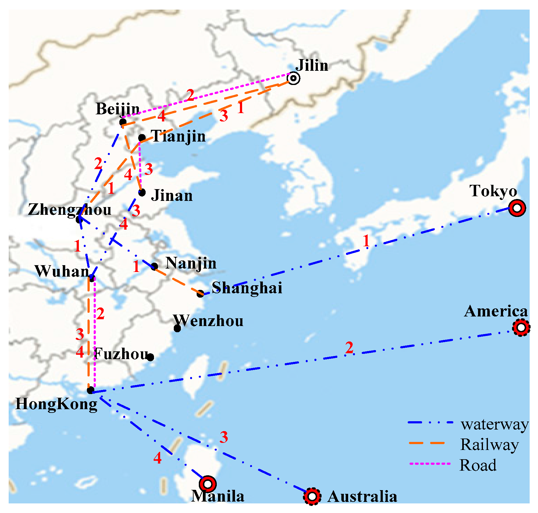
| Stage | Stage 1 | Stage 2 | Stage 3 | Stage 4 | Stage 5 |
|---|---|---|---|---|---|
| Nodes | Hong Kong (1) Fuzhou (2) Wenzhou (3) Shanghai (4) | Wuhan (1) Nanjing (2) | Zhengzhou (1) Jinan (2) | Beijing (1) Tianjin (2) | Jilin (1) |
| Sourcing Place | Tokyo | America | Australia | Manila |
|---|---|---|---|---|
| Supply/TEU | 80 | 50 | 50 | 120 |
| Mode | Waterway | Railway | Road | |
|---|---|---|---|---|
| Transportation cost ($/TEU-km) | 0.2 (Ship) | 0.18 (Barge) | 0.5 | 2 |
| Carbon emission cost ($/TEU-km) | 0.018 (Ship) | 0.015 (Barge) | 0.03 | 0.05 |
| Average speed (km/h) | 40 (Ship) | 30 (Barge) | 70 | 70 |
| Solution | Tokyo | America | Australia | Manilas | TTC/$ | MFT/h | CEC/$ | Feasibility (Yes/No) |
|---|---|---|---|---|---|---|---|---|
| 1 | 1-4-2-1-1-1-2-2-2 | 1-1-3-2-1-1-1-1-3 | 1-1-2-2-1-2-3-2-2 | 1-1-2-2-1-2-2-1-2 | 110,799 | 601 | 2330 | Yes |
| 2 | 1-1-2-2-1-2-2-2-2 | 1-1-2-2-1-1-3-2-3 | 1-1-2-2-1-1-2-2-2 | 1-1-2-2-1-2-2-2-2 | 99,097 | 614 | 2041 | Yes |
| 3 | 1-1-2-1-1-2-2-2-2 | 1-1-2-2-1-2-3-1-3 | 1-1-2-2-1-2-2-1-2 | 1-1-2-1-1-2-2-1-2 | 92,188 | 617 | 1854 | Yes |
| 4 | 1-4-2-2-1-2-2-1-2 | 1-1-2-2-1-1-2-2-2 | 1-1-2-1-1-2-3-2-2 | 1-1-2-2-1-2-2-1-2 | 92,141 | 662 | 1850 | Yes |
| 5 | 1-1-2-2-1-2-3-2-2 | 1-1-2-2-1-1-3-1-3 | 1-1-2-1-1-2-2-1-2 | 1-1-2-2-1-2-2-1-2 | 103,661 | 610 | 2106 | Yes |
© 2017 by the authors. Licensee MDPI, Basel, Switzerland. This article is an open access article distributed under the terms and conditions of the Creative Commons Attribution (CC BY) license (http://creativecommons.org/licenses/by/4.0/).
Share and Cite
Ji, S.-f.; Luo, R.-j. A Hybrid Estimation of Distribution Algorithm for Multi-Objective Multi-Sourcing Intermodal Transportation Network Design Problem Considering Carbon Emissions. Sustainability 2017, 9, 1133. https://doi.org/10.3390/su9071133
Ji S-f, Luo R-j. A Hybrid Estimation of Distribution Algorithm for Multi-Objective Multi-Sourcing Intermodal Transportation Network Design Problem Considering Carbon Emissions. Sustainability. 2017; 9(7):1133. https://doi.org/10.3390/su9071133
Chicago/Turabian StyleJi, Shou-feng, and Rong-juan Luo. 2017. "A Hybrid Estimation of Distribution Algorithm for Multi-Objective Multi-Sourcing Intermodal Transportation Network Design Problem Considering Carbon Emissions" Sustainability 9, no. 7: 1133. https://doi.org/10.3390/su9071133
APA StyleJi, S.-f., & Luo, R.-j. (2017). A Hybrid Estimation of Distribution Algorithm for Multi-Objective Multi-Sourcing Intermodal Transportation Network Design Problem Considering Carbon Emissions. Sustainability, 9(7), 1133. https://doi.org/10.3390/su9071133