CO₂ Emission Performance, Mitigation Potential, and Marginal Abatement Cost of Industries Covered in China’s Nationwide Emission Trading Scheme: A Meta-Frontier Analysis

Abstract

China’s nationwide emission trading scheme (CN-ETS) is scheduled to be launched in 2017. It is of great urgency and necessity to obtain a good understanding of the participating sectors of CN-ETS in terms of energy utilization and CO₂ emissions. In this regard, it should be noted that the findings may be biased without taking industry heterogeneity into consideration. To this end, a meta-frontier framework with the directional distance function is employed to estimate the CO₂ emission performance (CEP), mitigation potential (MP), and marginal abatement cost (MAC) at sector levels under the meta-frontier and the group-frontier. The results indicate that significant disparities in the CEP, MP, and MAC exist under both frontiers among various sectors, and the sectoral distributions of CEP, MP, and MAC are found to be different between the two frontiers. Additionally, the differences between the two frontiers in terms of CEP, MP, and MAC are considerable, and exhibit unequal distributions among these sectors. Notably, MAC under both frontiers and the difference between them are found to be significantly correlated with the carbon intensity. Finally, policy implications are provided for the government and participating enterprises, respectively.

1. Introduction

With climate change becoming an increasingly serious issue, the reduction of carbon dioxide (CO₂) emissions has attracted extensive attention worldwide. As the greatest CO₂ emitter in the world [1,2], China has shown its determination for developing a low-carbon economy and promised to abate its CO₂ emissions per unit of gross domestic product (GDP) (i.e., carbon intensity) by 40–45% by 2020 compared with that in 2005 [3]. Further, China set the latest target of abating carbon intensity by 18% by 2020, with 2015 as the reference year [4]. In order to achieve the above international commitments for mitigating CO₂ emissions, China’s National Development and Reform Commission (NDRC) has launched seven pilot emission trading schemes (ETS) since 2013 [5], which are specifically located in Shenzhen, Guangdong, Shanghai, Beijing, Tianjin, Chongqing, and Hubei. These regional carbon markets are considered as experimental explorations for the establishment of China’s nationwide emission trading scheme (CN-ETS), which is scheduled to be launched in 2017. It is reported the CN-ETS will cover seven emission-intensive industries, including paper making, electricity generation, metallurgy, non-ferrous metals, building materials, the chemical industry, and the aviation service industry [6].

In the context of achieving the construction and operation of CN-ETS, it is of great urgency and necessity to obtain a good understanding of the participating sectors in terms of energy utilization and CO₂ emissions [7]. In this regard, estimating the CO₂ emission performance (CEP), mitigation potential (MP), and marginal abatement costs (MAC) for these sectors can provide valuable information for the governments and participating enterprises. From the perspective of the government, a good knowledge of CEP, MP, and MAC could help design appropriate market mechanisms for the CN-ETS, e.g., the estimated MAC may be used as a reference for carbon pricing [8,9]. On the other hand, a comprehensive acquaintance of MAC among the participating sectors could help the participating enterprises to determine the best mitigation strategies [10]. Moreover, to the best knowledge of the authors, there have been few studies on the CEP, MP, and MAC of the sectors covered in the CN-ETS, and this paper aims to fill this research gap.

Additionally, it is accepted that there exists significant heterogeneity in terms of the production technology among various sectors [11], which is regarded as an obstacle to the objective evaluation of CEP, MP, and MAC [12]. Therefore, taking the technology heterogeneity into consideration, we employ a joint framework consisting of the directional distance function (DDF) and meta-frontier analysis to estimate CEP, MP, and MAC under the meta-frontier and the group-frontier, respectively. Following this, we investigate the sectoral distributions of CEP, MP, and MAC under both frontiers, and analyze the differences between the two frontiers at sector levels. Finally, several policy recommendations for the CN-ETS are made based on the conclusions. The rest of the paper proceeds as follows: Section 2 provides a literature review. Section 3 introduces the methods and materials. Section 4 presents the empirical results and discussion. Section 5 draws conclusions and policy implications.

2. Literature Review

DDF, theorized and developed by Chung et al. [13] and Chambers et al. [14,15], has been widely employed to study energy and environmental issues [16,17,18,19,20]. The main advantage of the DDF is that it can achieve the expansion of desirable outputs and reduction of undesirable outputs (e.g., CO₂), simultaneously [18]. Generally, two estimation techniques are often employed to estimate the DDF, namely the parametric and non-parametric methods. Compared with the former, the non-parametric technique does not need to pre-determine any functional and parametric forms, thereby avoiding the impacts of subjective factors on the results [17]. In this regard, the data envelopment analysis (DEA), a well-developed nonparametric frontier tool, is often combined with DDF to evaluate CEP [21,22,23], MP [9,24], and MAC [25,26,27]. For instance, Watanabe and Tanaka [21] employed the DEA-DDF to estimate the environmental performance for China’s industrial sector at province levels from 1994 to 2002. Liu et al. [26] evaluated the carbon emission performance and marginal abatement cost for provinces in China by using a non-parametric DDF. Additionally, the same method was applied by Wei et al. [9] to measure the reduction potential of CO₂ emissions for the thermal power plants in China’s Zhejiang province.

Considering the technology heterogeneity across decision making units (DMUs), Battese et al. [28] and O’Donnell et al. [29] incorporated the meta-frontier approach into DDF to formulate a joint framework. In the framework, DMUs with different production technologies are classified into several groups in which DMUs are deemed to be homogeneous, and then evaluated under the meta-frontier and the group-frontier, respectively. Recently, this combined methodology has been widely applied in the energy and environmental field [30,31,32,33,34,35,36,37,38,39]. For instance, using the combined method of DDF and the meta-frontier approach, Lin et al. [33] evaluated the environmental performance of 63 countries during the period from 1981 to 2005. Further, Zhang et al. [34] proposed a meta-frontier non-radial DDF by combining the meta-frontier approach with the non-radial DDF, and used it to assess the energy and CO₂ emission performance of electricity generation in Korea. Furthermore, the model was applied by Yao et al. [36] to estimate China’s energy efficiency, carbon emission performance, and mitigation potential at regional levels. Additionally, based on the same model, Li and Song [38] constructed a green development growth index to assess China’s green development at province levels.

The literature on energy and environmental issues is abundant at industry levels [7,10,27,40,41]. For instance, Lee and Zhang [27] measured the reduction potential and marginal abatement cost of CO₂ emissions for 30 of China’s manufacturing industries. Yuan et al. [40] estimated the shadow prices of CO₂ emissions for China’s industrial sectors with the use of non-parametric DDF. Teng et al. [41] employed multiple methods to derive the marginal abatement cost curves for China’s energy-intensive industries. Zhou et al. [10] applied multiple distance function approaches to approximate the shadow prices of CO₂ emissions for Shanghai’s industrial sectors. Xiao et al. [7] estimated the marginal abatement costs of CO₂ emissions for China’s industrial sectors during 2005–2011 by using a parametric DDF. Notably, it is found that the above studies mainly focus on the industrial sectors, while a comprehensive investigation on the participating sectors of CN-ETS has not been conducted. Furthermore, to the best of our knowledge, few studies take the industry heterogeneity into account, in addition to Xie et al. [11] and Chung and Heshmati [12]. In this context, we attempt to perform an empirical study on the participating sectors of CN-ETS in terms of CEP, MP, and MAC, taking into consideration the industry heterogeneity.

3. Methods and Materials

3.1. Environmental Production Technology

Consider a productive process in which various inputs of energy and non-energy resources are utilized to jointly produce desirable outputs and undesirable outputs. Mathematically, the joint production can be presented as Equation (1), which is the so-called environmental production technology.

$$P\left(x\right)=\left\{\left(y,b\right) :x can produce \left(y,b\right)\right\}$$

(1)

where $x\in {\Re }_{+}^I$ denotes the input vector, $y\in {\Re }_{+}^J$ denotes the desirable output vector, and $b\in {\Re }_{+}^K$ denotes the undesirable output vector. Notably, in the joint-production process, the inputs and the desirable outputs are usually presumed to be strongly disposable, while the undesirable outputs are weakly disposable.

3.2. Directional Distance Function

The directional distance function (DDF) has been widely utilized to characterize the environmental production technology. Compared with traditional distance functions, DDF can achieve the simultaneous extension of desirable outputs and shrinkage of undesirable outputs, which can be mathematically defined in Equation (2).

$$\overrightarrow{D}\left(x,y,b;g_y,g_b\right)=max\left\{\beta :\left(y+\beta g_y,b+\beta g_b\right)\in P\left(x\right)\right\}$$

(2)

where $\left(g_y, g_b\right)$ is the direction vector indicating the scale directions for the desirable outputs and undesirable outputs, which is generally specified as $\left(y, -b\right)$. β is the outcome of DDF that estimates the greatest extent to which y and b can be respectively expanded and reduced given x.

Following Boyd et al. [42], the non-parametric DEA-DDF with constant returns to scale (CRS) is presented as follows:

$$\begin{array}{c}\overrightarrow{D}\left(x,y,b;y,-b\right)=\max {\beta }_0\\ {\displaystyle \sum }_{j=1}^N{\lambda }_j{x}_j\le x_0\\ {\displaystyle \sum }_{j=1}^N{\lambda }_j{y}_j\ge \left(1+{\beta }_0\right)y_0\\ {\displaystyle \sum }_{j=1}^N{\lambda }_j{b}_j=\left(1-{\beta }_0\right)b_0\\ {\beta }_0\ge 0, {\lambda }_j\ge 0\end{array}$$

(3)

where $x_0, y_0, b_0$, respectively, denote the inputs, desirable outputs, and undesirable outputs for the observed production unit, and ${\lambda }_j$ is the intensity variable. Notably, the equal sign of the third constraint in Equation (3) reflects the weak disposability assumption of the undesirable outputs.

3.3. Meta-Frontier and Group-Frontier

Considering the existence of heterogeneity among various sectors in terms of energy utilization and carbon emissions, we thereby incorporate a meta-frontier analysis into the above DDF. Suppose N DMUs (industries in this paper) can be classified into $I \left(I\ge 1\right)$ groups. The number of DMUs in the $i$th group is $N_i\left(i =1, 2, \dots , I\right)$, and ${\displaystyle \sum }_{i=1}^I{N}_i=1$. Thus, the environmental production technologies of the meta-frontier and group-frontier can be described as follows:

$$P^M\left(x\right)=\left\{\left(y,b\right) : x can produce \left(y,b\right)\right\}$$

(4)

$$P^{G-i}\left(x\right)=\left\{\left(y,b\right) : x can produce \left(y,b\right)\right\}, i=1,2,\dots ,I$$

(5)

where both $P^M\left(x\right)$ and $P^{G-i}\left(x\right)$ satisfy the assumptions of disposability mentioned earlier, and $P^M\left(x\right)$ consists of all the $P^{G-i}\left(x\right)\left(i=1,2,\dots ,I\right):P^M\left(x\right)=\left\{P^{G-1}\left(x\right){{\displaystyle \cup }}^{\text{}}{P}^{G-i}\left(x\right){{\displaystyle \cup }}^{\text{}}\dots {{\displaystyle \cup }}^{\text{}}{P}^{G-I}\left(x\right)\right\}$, namely, $P^M\left(x\right)$ includes all DMUs and envelops all group frontiers.

Applying the DDF depicted in Equation (2) to specify Equations (4) and (5), we can obtain the meta-frontier DDF and the $i$th group-frontier DDF:

$${\overrightarrow{D}}^M\left(x,y,b;g_y,g_b\right)=max\left\{{\beta }^M:\left(y+{\beta }^M{g}_y,b+{\beta }^M{g}_b\right)\in P^M\left(x\right)\right\}$$

(6)

$${\overrightarrow{D}}^{G-i}\left(x,y,b;g_y,g_b\right)=max\left\{{\beta }^{G-i}:\left(y+{\beta }^{G-i}{g}_y,b+{\beta }^{G-i}{g}_b\right)\in P^{G-i}\left(x\right)\right\}, i=1,2,\dots ,I$$

(7)

Finally, we employ Equation (3) to estimate the DDF values under the meta-frontier $\left({\beta }^M\right)$ and group-frontier $\left({\beta }^{G-i}\right)$, respectively.

3.4. CO₂ Emission Performance and Mitigation Potential

According to Hu and Wang [43], Zhou and Ang [44], and Choi et al. [45], the CEP can be measured by the ratio of target CO₂ emissions to the actual CO₂ emissions:

$${\mathrm{CEP}}_j=\frac{C_j-{\beta }_j{C}_j}{C_j}=1-{\beta }_j$$

(8)

where ${\mathrm{CEP}}_j$, $C_j$, and ${\beta }_j$ denote the CEP, actual CO₂ emissions, and DDF value of ${\mathrm{DMU}}_j$, respectively. In addition, ${\beta }_j{C}_j$ denotes the excessive CO₂ emissions of ${\mathrm{DMU}}_j$ compared with the frontier, which is considered as achievable emission reductions. Thus, the MP of ${\mathrm{DMU}}_j$ can be measured by Equation (9):

$${\mathrm{MP}}_j=\frac{{\beta }_j{C}_j}{C_j}\times 100\%={\beta }_j\times 100\%$$

(9)

where ${\mathrm{MP}}_j$ denotes the MP of ${\mathrm{DMU}}_j$, and the sum of ${\mathrm{CEP}}_j$ plus ${\mathrm{MP}}_j$ equals 1, which implies that a greater reduction potential signifies a worse environmental performance of the observation.

3.5. Shadow Price

The shadow price is often utilized to approximate the marginal abatement cost of undesirable outputs, which is generally read as the opportunity cost of eliminating one extra unit of undesirable output in terms of lost desirable outputs in the production process. In this context, Färe and Grosskopf [16] developed the duality relationship between the distance function and revenue function, which is of great significance for the derivation of the shadow price of undesirable outputs. With the use of the Lagrangian technique and the envelope theorem, the shadow price of undesirable outputs is derived as follows:

$$p^b=-p^y\times \frac{\partial \overrightarrow{D}\left(x,y,b;g_y,g_b\right)/\partial b}{\partial \overrightarrow{D}\left(x,y,b;g_y,g_b\right)/\partial y}$$

(10)

Noticing the deficiency that different observations sharing the same frontier point enjoy at the same shadow price, Lee et al. [46] thereby incorporated an inefficiency factor into Equation (8) and reformulated the shadow-pricing equation as:

$$p^b=-p^y\times \frac{\partial \overrightarrow{D}\left(x,y,b;g_y,g_b\right)/\partial \left({\sigma }_{b}b\right)}{\partial \overrightarrow{D}\left(x,y,b;g_y,g_b\right)/\partial ({\sigma }_{y}y)}\times \frac{{\sigma }_b}{{\sigma }_y}$$

(11)

where $p^y$ and $p^b$, respectively denote the shadow prices of the desirable and undesirable outputs. According to Färe et al. [47], $p^y$ is usually assumed to equal its market price (i.e., 1). ${\sigma }_y,{\sigma }_b$ are the inefficiency factors and ${\sigma }_b/{\sigma }_y$ equals $\left(1-\beta )/(1+\beta \right)$.

3.6. Materials

3.6.1. Sectors and Variables

It is reported that the CN-ETS will cover the emission-intensive industries of paper making, electricity generation, metallurgy, non-ferrous metals, building materials, the chemical industry, and the aviation service industry [6]. According to the Standard Industrial Classification formulated by the National Bureau of Statistics of China (NBSC), the seven industries covered in the CN-ETS can be further divided into 39 sectors. Furthermore, according to the carbon intensity, the 39 sectors can be classified into three groups: high-carbon, medium-carbon, and low-carbon groups, and each group consists of 13 sectors. The specific sectors of the three groups are listed in

Table 1. Specific sectors and codes for high-, medium-, and low-carbon groups.

High-Carbon Group	Medium-Carbon Group	Low-Carbon Group
Electricity Generation and Supply (S1)	Manufacture of Glass Products (S14)	Manufacture of Paper (S27)
Pressing of Steel (S2)	Manufacture of Ceramics Products (S15)	Manufacture of Paper Products (S28)
Smelting of Steel (S3)	Manufacture of Glass Fiber Products (S16)	Manufacture of Paper Pulp (S29)
Casting of Ferrous Metals (S4)	Manufacture of Glass (S17)	Manufacture of Synthetic Fibers (S30)
Smelting of Ferroalloy (S5)	Manufacture of Raw Chemical Materials (S18)	Manufacture of Fiber Materials (S31)
Smelting of Iron (S6)	Manufacture of Special Chemical Products (S19)	Pressing of Non-ferrous Metals (S32)
Processing of Petroleum (S7)	Manufacture of Synthetic Materials (S20)	Smelting of Common Non-ferrous Metals (S33)
Processing of Coking (S8)	Manufacture of Fertilizers (S21)	Smelting of Non-ferrous metal alloy (S34)
Manufacture of Tile and Construction stone (S9)	Manufacture of Paints and Pigments (S22)	Smelting of Precious Metals (S35)
Manufacture of Cement and Limestone Products (S10)	Manufacture of Common Chemical Products (S23)	Smelting of Rare Earth Metals (S36)
Manufacture of Cement and Limestone (S11)	Manufacture of Pesticides (S24)	Casting Pressing of Non-ferrous Metals (S37)
Manufacture of other Non-metallic Mineral Products (S12)	Manufacture of Explosives and Fireworks (S25)	Manufacture of Plastics Products (S38)
Manufacture of Fireproof Materials (S13)	Civil Aviation Services (S26)	Manufacture of Rubber Products (S39)

Note: sector’s carbon intensity gradually decreases from S1 to S39.

.

Following the common practice in the literature, this paper selects five variables as the input- output indicators. Specifically, three variables of capital stock, labor employment, and energy consumption serve as the inputs, while the industrial value added (IVA) and CO₂ emissions are viewed as the desirable output and the undesirable output, respectively. The input-output variables are summarized in

Table 2. Variables of inputs and outputs.

Category	Variable	Unit
Input	Capital	100 million Yuan
	Labor	10 thousand persons
	Energy	10 thousand tons of coal equivalent (10,000 tce)
Desirable output	IVA	100 million Yuan
Undesirable output	CO2 emission	10 thousand tons

Note: Yuan denotes Chinese currency.

.

3.6.2. Data

A statistical description of the input-output data is shown in

Table 3. Descriptive statistics of input-output data (2014 and 2017).

Year	Items	Inputs			Desirable Output	Undesirable Output
		Capital	Labor	Energy	IVA	CO2
2014	Mean	4394.54	66.93	7393.14	2284.41	25,858.95
	Std. dev.	10678.39	64.43	22,921.26	2857.27	87,583.80
	Max	66,386.48	259.51	138,403.59	13,761.05	536,897.12
	Min	55.01	1.59	14.95	37.31	55.93
2017	Mean	6108.10	69.16	8418.21	2839.78	28,994.29
	Std. dev.	14,842.20	66.58	26,099.32	3551.90	98,203.14
	Max	92,272.49	268.17	157,593.40	17,106.51	601,994.73
	Min	76.46	1.64	17.02	46.38	62.71

Note: due to limitations of statistical data, the data in this paper only contain industrial enterprises above designated size.

, and a detailed description of the data sources of each variable is provided below.

Capital stock is generally estimated by the Perpetual Inventory Method (PIM), which requires the data of the initial capital stock and industrial capital depreciation rate. However, due to the limitations of statistical data, these data also need to be estimated. Thus, to decrease the deviation from data estimation, we adopt an alternative approach of taking the net value of fixed assets as the capital stock [48], which are collected from the “China Industrial Economic Statistical Yearbook 2015 [49]”. Moreover, the data of the “Civil Aviation Services (S26)” are collected from “From the Statistical View of Civil Aviation 2015 [50]”.

Labor employment is directly collected from the “China Industrial Economic Statistical Yearbook 2015 [49]” and “From the Statistical View of Civil Aviation 2015 [50]”.

Energy consumption denotes the comprehensive consumption of end-use energy, which includes 17 fuels of raw coal, cleaned coal, other washed coal, coke, coke oven gas, other gas, other coking products, crude oil, gasoline, kerosene, diesel oil, fuel oil, liquefied petroleum gas (LPG), refinery gas, other petroleum products, natural gas, and liquefied natural gas (LNG). The related data are obtained from the “China Energy Statistical Yearbook [51]” and “From the Statistical View of Civil Aviation 2015 [50]”. All kinds of energy usages are converted into standard coal equivalents with the use of conversion factors which are provided in Appendix IV of the China Energy Statistical Yearbook.

Considering that IVA cannot be directly gathered from relevant statistical yearbooks since 2008, we calculate the data in 2014 by multiplying those in 2007 with the growth rates of the industrial added value, which are acquired from the National Data Website [52]. Notably, the industrial added value of the Civil Aviation Service industry is converted from the main business income, by multiplying the ratio of the industrial added value of the entire industrial sector to the corresponding main business income. The main business income of the Civil Aviation Service industry is gathered from “From the Statistical View of Civil Aviation 2015 [52]”.

CO₂ emissions are generally estimated with the reference approach of the Intergovernmental Panel on Climate Change (IPCC), due to the lack of official statistical data on CO₂ emissions in China. Therefore, this paper also adopts the approach to estimate CO₂ emissions with the use of energy usage data:

$$C{O}_2 emissions={{\displaystyle \sum }}_i{E}_i\times NC{V}_i\times CE{F}_i\times CO{F}_i\times \left(44/12\right)$$

(12)

where $E_i$ denotes the final usage of energy source $i$; $NC{V}_i\left(\mathrm{net}\mathrm{caloric}\mathrm{value}\right)$, $CE{F}_i\left({\mathrm{CO}}_2\mathrm{emission}\mathrm{factor}\right)$, and $CO{F}_i\left({\mathrm{CO}}_2\mathrm{oxidation}\mathrm{factor}\right)$ denote the heat equivalent, the CO₂ emission factor, and the CO₂ oxidation factor, respectively. $44/12$ is the ratio of the CO₂ molecular weight (44) to the C atomic weight (12), which is named the CO₂ gasification coefficient.

Based on the economic development strategy and mitigation policy objectives which are included in “China’s 12th Five Year Plan [53]”, “China’s 13th Five Year Plan [4]”, and the “Industrial Action Plan on Climate Change (2012–2020) [54]”, we calculate the annual growth rates of capital stock, labor employment, energy consumption, IVA, and CO₂ emissions. For instance, the annual average growth rates of energy consumption and CO₂ emissions are calculated based on the projected goals set for the energy consumption reduction per unit of GDP and CO₂ emissions reduction per unit of GDP. Additionally, the annual growth rates of the capital stock and labor employment are assumed to be unchanged during the two periods [55].

Table 4. Annual growth rate of input and output variables.

Annual Growth Rate	2011–2015	2016–2020
${\phi }^k$	11.59%	11.59%
${\phi }^l$	1.11%	1.11%
${\phi }^e$	6.53%	3.43%
$\mu$	9.60%	6.50%
$\eta$	6.05%	2.75%

Note: ${\phi }^k, {\phi }^l,\mathrm{and}{\phi }^e$ denote the annual growth rate of capital stock, labor employment, and energy consumption, while $\mu$ and $\eta$ denote that of IVA and CO₂ emission.

reports the annual growth rates of the variables. By multiplying the respective annual growth rate, the input-output data in 2014 are used to forecast those in 2017, and the results are listed in Table 3.

4. Results and Discussions

In this section, we first report the estimates of DDF values ($\beta$), CO₂ emission performance (CEP), mitigation potential (MP), and marginal abatement cost (MAC) under the meta-frontier and group-frontier at group levels. Then, we investigate the sectoral distributions of CEP, MP, and MAC under both frontiers, and analyze the differences between the two frontiers in terms of the CEP, MP, and MAC at sector levels.

4.1. Statistical Summary of Estimates

4.1.1. DDF Values

DDF values under the meta-frontier (${\beta }^M$) and the group-frontier (${\beta }^G$) are estimated by combining Equation (3) with Equations (6) and (7), respectively, and the results are listed in

Table 5. Estimates of DDF values.

	Groups	N	Min	Max	Mean	Std. Dev.
Meta-frontier	High-carbon	13	0.000	0.888	0.688	0.214
	Medium-carbon	13	0.000	0.840	0.672	0.211
	Low-carbon	13	0.000	0.635	0.271	0.216
	Total	39	0.000	0.888	0.544	0.285
Group-frontier	High-carbon	13	0.000	0.687	0.234	0.217
	Medium-carbon	13	0.000	0.532	0.169	0.209
	Low-carbon	13	0.000	0.635	0.271	0.216
	Total	39	0.000	0.687	0.225	0.213

. From the table, it can be observed that ${\beta }^M$ and ${\beta }^G$ vary from 0 to 0.888 and from 0 to 0.687, respectively. Moreover, the mean values of ${\beta }^M$ are generally larger than those of ${\beta }^G$. From the perspective of total sectors, the average ${\beta }^M$ is found to be 0.544, which is more than twice that of ${\beta }^G$ (0.225), indicating that there is a significant difference. Additionally, the differences in the average DDF value between the two frontiers are found to be considerable at group levels, especially for the high-carbon and medium-carbon groups. Specifically, the average ${\beta }^M$ (0.688) of the high-carbon group is found to be almost three times that of ${\beta }^G$ (0.234). Further, the average DDF value of the medium-carbon group varies between the meta-frontier and group-frontier at greater levels, which is found to jump from 0.169 to 0.672. As for the low-carbon group, the difference between the two frontiers could be neglected. Notably, there are significant differences among the DDF values of the three groups when the meta-frontier is used as the basis of evaluation, while relatively moderate distinctions are observed when using the group frontiers.

4.1.2. CO₂ Emission Performance

Table 6. Estimates of CO₂ emission performance.

	Groups	N	Min	Max	Mean	Std. Dev.
Meta-frontier	High-carbon	13	0.112	1.000	0.312	0.214
	Medium-carbon	13	0.160	1.000	0.328	0.211
	Low-carbon	13	0.365	1.000	0.729	0.216
	Total	39	0.112	1.000	0.456	0.285
Group-frontier	High-carbon	13	0.313	1.000	0.766	0.217
	Medium-carbon	13	0.468	1.000	0.831	0.209
	Low-carbon	13	0.365	1.000	0.729	0.216
	Total	39	0.313	1.000	0.775	0.213

reports the estimates of CO₂ emission performance under the meta-frontier (MCEP) and the group-frontier (GCEP). From the table, it is found that MCEP and GCEP vary from 0.112 to 1 and from 0.313 to 1, respectively. Moreover, the mean values of GCEP are generally higher than those of MCEP. From the perspective of total sectors, the average GCEP is found to be 0.775, while that under the meta-frontier is only 0.456, which indicates that there is a significant difference. Additionally, the differences in the average CEP scores between the two frontiers are found to be considerable at group levels, especially for the high-carbon and medium-carbon groups. Specifically, the average GCEP (0.766) of the high-carbon group is found to be more than twice that of MCEP (0.312). Similarly, the average CEP of the medium-carbon group is found to jump from 0.328 to 0.831, which is an increase of 153%. As for the low-carbon group, the difference between the two frontiers could be neglected. Notably, there are significant differences among the CEP scores of the three groups when the meta-frontier is used as the basis of evaluation, while relatively moderate distinctions are found when using the group frontiers.

4.1.3. Mitigation Potential

Table 7. Estimates of mitigation potential.

	Groups	N	Min	Max	Mean	Std. Dev.
Meta-frontier	High-carbon	13	0.0%	88.8%	68.8%	0.214
	Medium-carbon	13	0.0%	84.0%	67.2%	0.211
	Low-carbon	13	0.0%	63.5%	27.1%	0.216
	Total	39	0.0%	88.8%	54.4%	0.285
Group-frontier	High-carbon	13	0.0%	68.7%	23.4%	0.217
	Medium-carbon	13	0.0%	53.2%	16.9%	0.209
	Low-carbon	13	0.0%	63.5%	27.1%	0.216
	Total	39	0.0%	68.7%	22.5%	0.213

reports the estimates of Mitigation Potential under the meta-frontier (MMP) and the group-frontier (GMP). From the table, it can be observed that MMP and GMP vary from 0% to 88.8% and from 0% to 68.7%, respectively. Moreover, the mean values of MMP are generally higher than those of GMP. From the perspective of total sectors, the average MMP is found to be 54.4%, which is more than twice the mean value of GMP (22.5%), indicating that there is a significant difference. Additionally, the differences in the average MP values between the two frontiers are found to be considerable at group levels, especially for the high-carbon and medium-carbon groups. Specifically, the average MMP of the high-carbon group (68.8%) is found to be almost three times that of GMP (23.4%). Further, the average MP value of the medium-carbon group varies between the meta-frontier and group-frontier at greater levels, which is found to jump from 16.9% to 67.2%. As for the low-carbon group, the difference between the two frontiers could be neglected. Notably, there are significant differences among the MP values of the three groups when the meta-frontier is used as the basis of evaluation, while relatively moderate distinctions are observed when using the group frontiers.

4.1.4. Marginal Abatement Cost

Table 8. Estimates of marginal abatement cost (unit: 10,000 Yuan per ton).

	Groups	N	Min	Max	Weighted Mean 1	Std. Dev.
Meta-frontier	High-carbon	13	0.024	0.246	0.050	0.054
	Medium-carbon	13	0.083	0.506	0.131	0.110
	Low-carbon	13	0.242	1.297	0.497	0.329
	Total	39	0.024	1.297	0.067	0.343
Group-frontier	High-carbon	13	0.016	0.147	0.040	0.033
	Medium-carbon	13	0.079	0.258	0.208	0.074
	Low-carbon	13	0.361	1.616	1.032	0.447
	Total	39	0.016	1.616	0.077	0.485

¹ Weight is the share of each sector’s emissions in the all.

reports the estimates of the marginal abatement cost under the meta-frontier (MMAC) and the group-frontier (GMAC). From the table, it is found that MMAC and GMAC vary from 240 to 12,970 Yuan/ton and from 160 to 16,160 Yuan/ton, respectively. From the perspective of the meta-frontier, the low-carbon group is found to have the highest weighted average MMAC of 4970 Yuan/ton, followed by the medium group with a value of 1310 Yuan/ton, and the high-carbon group is at the bottom, with a value of 500 Yuan/ton. On the other hand, the weighted average GMAC values of the three groups also follow the same order, which are found to be 10,320, 2080, and 400 Yuan/ton. The differences between the mean values of MMAC and GMAC at group levels are considerable, especially for the low-carbon group, which is found to have a twofold change in the values. Additionally, the average weighted MAC values of the total sectors under the group-frontier and the meta-frontier are found as 670 and 770 Yuan/ton, respectively. As a matter of fact, the sectors have to sacrifice relatively more IVA for reducing an additional unit of CO₂ emissions, if they are producing at the more efficient overall production frontier with relatively less mitigation potential. So, in general, marginal abatement costs are negatively correlated with the mitigation potential.

It is interesting to compare our MAC estimates with those of previous studies. A summary of MAC estimates is reported in

Table 9. Summary of MAC estimates (unit: Yuan per ton).

Studies	Methodology	Sample	Mean	Weighted Mean
Lee and Zhang (2012) [27]	IDF/P/T	30 Manufacturing industries, 2009	19.7	/
Yuan et al. (2012) [40]	DDF/N/DEA	24 Industrial sectors, 2004 and 2008	16,360	/
Zhou et al. (2015) [10]	MDF/N/T/Q	Shanghai’s industrial sectors	/	394.5–1906.1
Xie et al. (2016) [11]	DDF/N/Three-stage DEA	9 key industries, 2005–2014.	1345	/
Xiao et al. (2017) [7]	DDF/P/Q	39 industrial sectors, 2005–2011	13,131	3517
This paper	Meta-DDF/N/DEA	39 participating sectors of CN-ETS	3180 and 4240	670 and 770

Note: P = Parametric; N = Nonparametric; T = Translog functional form; Q = Quadratic functional form; IDF = Input distance function; DDF = Directional distance function; MDF = Multiple distance function; CN-ETS = China’s nationwide emission trading scheme.

. From the table, it can be observed that the estimates of the previous studies lie in different ranges. The different samples and approaches in these studies are the main reasons for the differences in the results. The results of this study are found to be apparently lower than those of Xiao et al. [7] in terms of the mean and weighted mean of MAC. This is reasonable because our study only covers the emission-intensive industries of the industrial sector, while Xiao et al. [7] consider all industrial sectors as research objects, which is more expensive to reduce emissions. Additionally, the significant disparity of the average MAC between Yuan et al. [40] and Xie et al. [11] can also be attributed to the difference in research objects.

4.2. Sectoral Analysis

4.2.1. Distribution Analysis

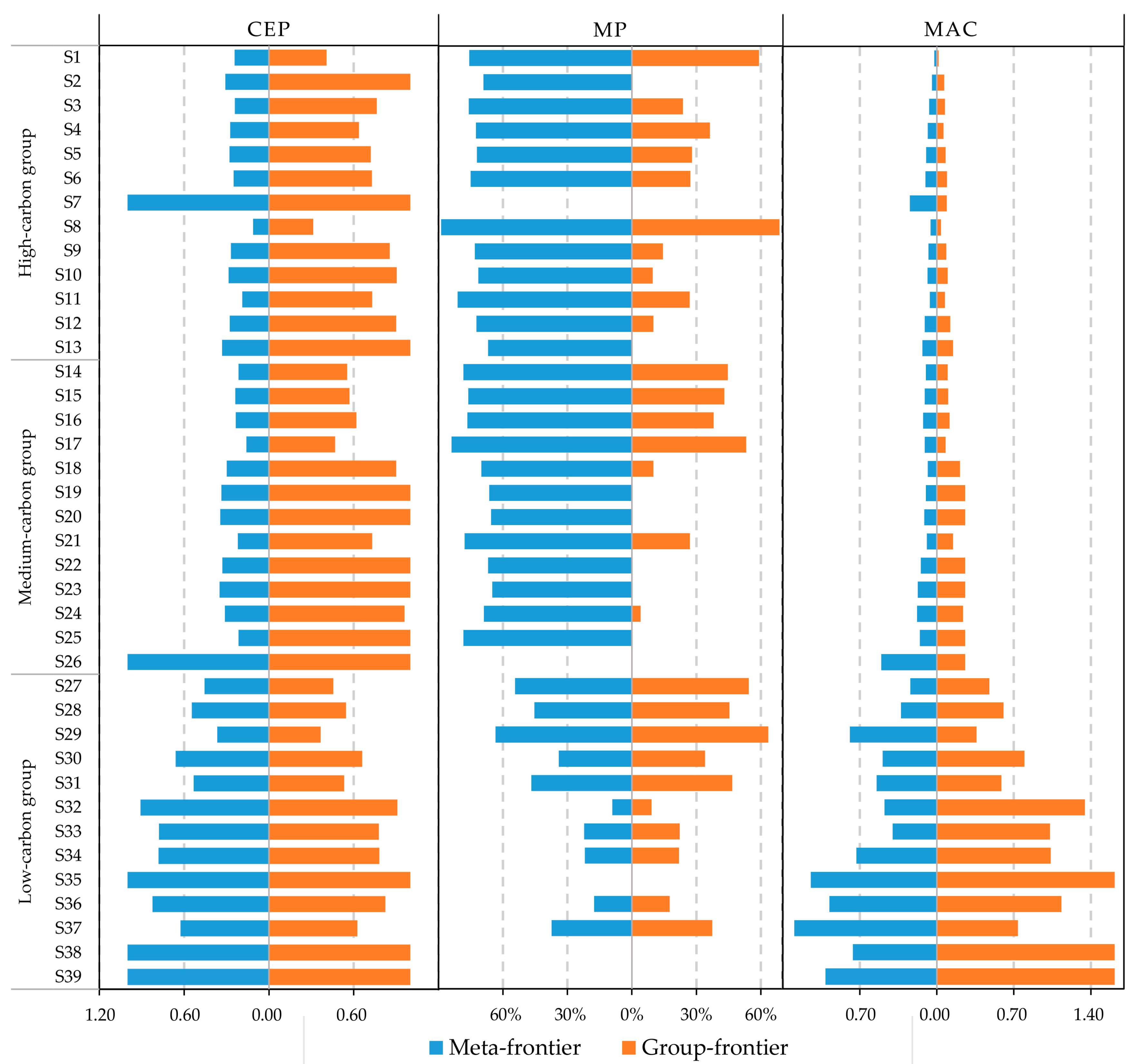
Figure 1 indicates the estimates of CEP, MP, and MAC under the meta-frontier and the group-frontier at the sector level. From the figure, we can observe that there exist significant disparities in the CEP, MP, and MAC under both frontiers among the 39 sectors. Specifically, from the meta-frontier perspective, the sectoral distribution of MCEP presents an increasing trend from S1 to S39 (i.e., the decreasing order of carbon intensity), while that of MMP presents the opposite tendency. Similarly, the sectoral distributions of GCEP and GMP show the upward and downward trends along with the decrease of carbon intensity in their respective groups, respectively. For instance, in the high-carbon group, the sectoral distribution of GCEP presents an increasing tendency from S1 to S13, while a decreasing trend is observed for GMP. On the other hand, it is found that both of the sectoral distributions of MMAC and GMAC present an increasing tendency from S1 to S39.

In light of this interesting phenomenon, we conducted a correlation analysis between MMAC, GMAC, and carbon intensity, respectively, and the results are listed in

Table 10. Correlation analysis.

Estimates	Items	Carbon Intensity
MMAC	Pearson correlation	−0.537 **
	Sig. (2-tailed)	0.000
	N	39
GMAC	Pearson correlation	−0.566 **
	Sig. (2-tailed)	0.000
	N	39
D_MAC	Pearson correlation	−0.320 *
	Sig. (2-tailed)	0.047
	N	39

** Correlation is significant at the 0.01 level (2-tailed); * Correlation is significant at the 0.05 level (2-tailed).

. According to the correlation results, there exists a significantly negative correlation (p = 0.000 < 0.01, Pearson’s r = −0.537) between carbon intensity and MMAC, which has been previously reported in the literature, such as in Zhou et al. [10]. Additionally, GMAC is also found to be significantly negatively correlated with carbon intensity (p = 0.000 < 0.01, Pearson’s r = −0.566).

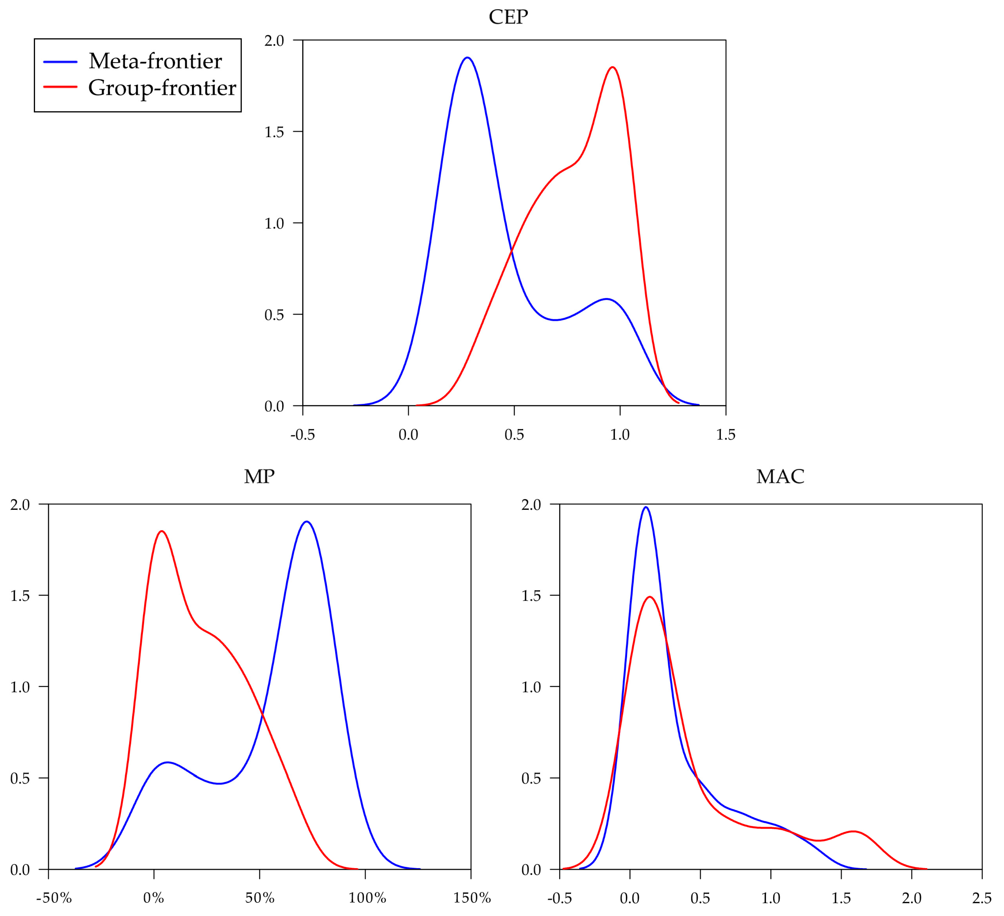
In order to provide an intuitive understanding of the distribution patterns of CEP, MP, and MAC, and make a comparison between the meta-frontier and the group-frontier, the kernel density curves of CEP, MP, and MAC under both frontiers are plotted based on the R-program. From Figure 2, it can be found that there exist some differences in the distribution patterns of CEP, MP, and MAC between the two frontiers. Specifically, the kernel curve of CEP moves rightward and the dispersion range of points become narrower when the evaluation basis switches from the meta-frontier to the group-frontier, which means an increase in the mean value and a decrease in the variance of CEP, respectively. In the meanwhile, the kernel curve of MP moves leftward and the dispersion range of points become narrower, which means that the mean value and the variance of MP both decrease. On the contrary, the kernel curve of MAC holds the position unchanged, but exhibits a significant decrease in the peak value and an expansion in the dispersion range of points when the evaluation basis changes, which jointly means a considerable increase in the variance of MAC.

4.2.2. Difference Analysis

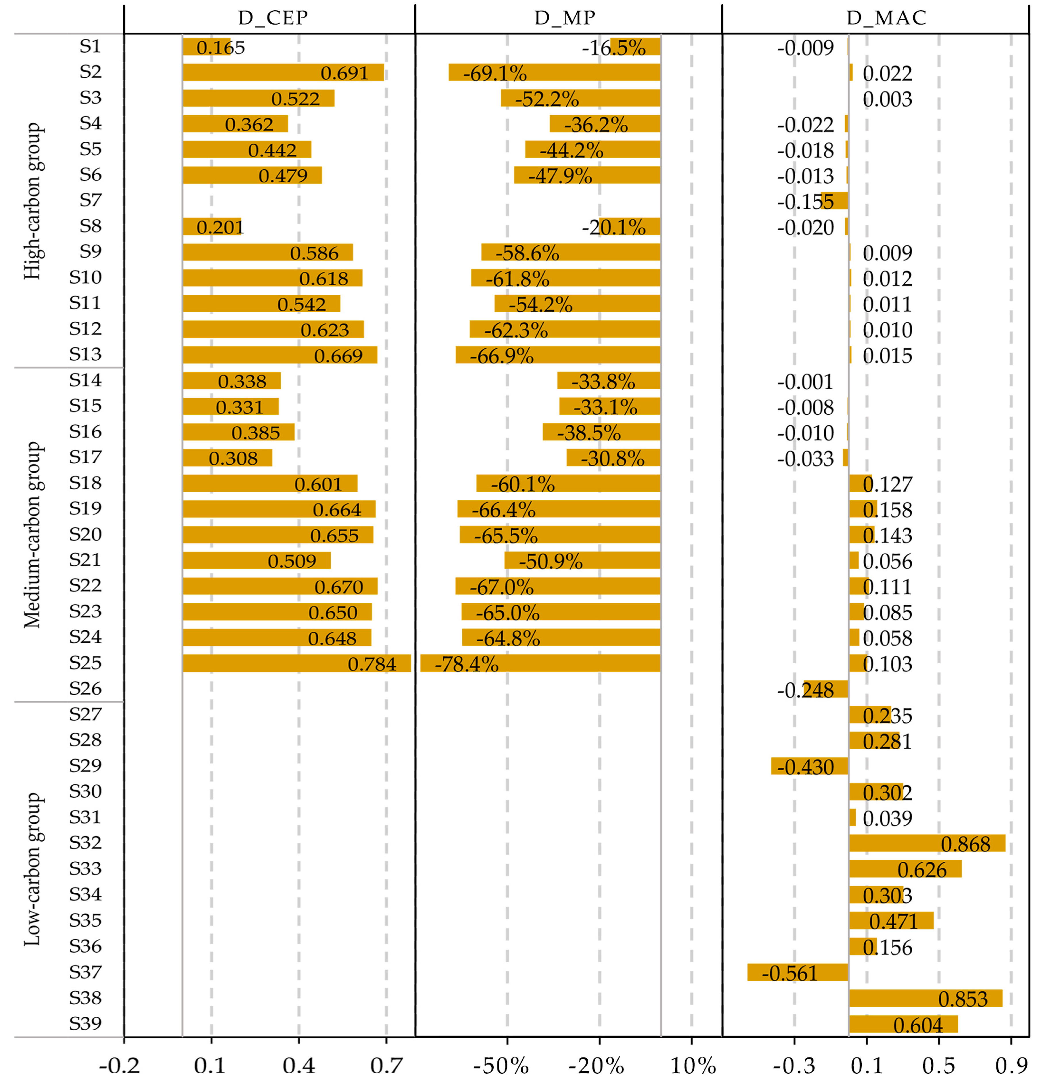
Figure 3 reports the differences in CEP, MP, and MAC between the meta-frontier and the group-frontier at sector levels. From the figure, we can observe that there exist significant disparities between the two frontiers in terms of CEP, MP, and MAC, and the differences exhibit unequal distributions among the 39 sectors. The difference in CEP (D_CEP) is found to be significant in the high-carbon and medium-carbon sectors. For instance, the D_CEP of Pressing of Steel (S2) is found to be 0.691. Similar results can be observed for sectors such as the Manufacture of Fireproof Materials (S13), Manufacture of Special Chemical Products (S19), and Manufacture of Explosives and Fireworks (S25). This means that there is significant technology heterogeneity between the meta-frontier and group-frontier for the two groups. Conversely, it is found that there is no difference in the low-carbon sectors, which may be attributed to the fact that low-carbon sectors play an important role in benchmarking efficiency levels under meta-frontier technologies, and thereby there are no technology gaps for the low-carbon sectors. Similarly, the difference in MP (D_MP) between the two frontiers is also found to be significant in the high-carbon and medium-carbon sectors, while the opposite is true for the low-carbon sectors.

On the other hand, the difference in MAC (D_MAC) exhibits a completely different situation, in which the D_MAC is found to be larger, equal to, and smaller than 0, depending on the observations. For instance, the Pressing of Non-ferrous Metals (S32) and Casting Pressing of Non-ferrous Metals (S37) are found to have the lowest and the highest D_MAC, with values of −5610 Yuan/ton and 8680 Yuan/ton, respectively. There is no definite relationship between the MMAC and GMAC of sectors; the MMAC of sectors can be larger, equal to, or smaller than the GMAC, depending on the relative slopes of the meta- and the group-frontiers, respectively [19]. However, as mentioned earlier, both MMAC and GMAC are significantly correlated with carbon intensity. Therefore, it is interesting to explore the relationship between D_MAC and carbon intensity. In this regard, the correlation analysis between D_MAC and carbon intensity was conducted, and the results are listed in Table 10. According to the correlation results, there is also a significantly negative correlation (p = 0.047 < 0.05, Pearson’s r = −0.320) between D_MAC and carbon intensity.

4.3. Discussions

In general, whether from the perspective of group levels or from the perspective of sector levels, it is found that there exist significant disparities in the CEP, MP, and MAC under both frontiers among various sectors. Additionally, the differences between the two frontiers in terms of CEP, MP, and MAC are considerable, and exhibit unequal distributions among the 39 sectors. This can be attributed to the significant heterogeneity of production technology among various sectors. Considering that carbon intensity is widely considered as the measurement of carbon emission efficiency, the industries with a relatively low carbon intensity are more efficient than those with a high carbon intensity in terms of energy utilization and carbon emissions. Thus, low-carbon sectors are found to have a higher CEP, less MP, and larger MAC than medium-carbon and high-carbon sectors.

As the most efficient DMUs, low-carbon sectors are found to play a more important role in benchmarking efficiency levels under the meta-frontier. In this case, no difference between the meta-frontier and the group-frontier for the low-carbon group in terms of CEP and MP exists, while the opposite is true for the medium-carbon and high-carbon sectors. As a result, considerable differences in the CEP and MP between the two frontiers are observed for the medium-carbon and high-carbon sectors. As for MAC, theoretically, the MMAC can be larger, equal to, or smaller than the GMAC, depending on the relative slopes of the meta-frontier and the group-frontier. Nevertheless, it is found that D_MAC has a significantly negative correlation with carbon intensity.

5. Conclusions and Policy Implications

CN-ETS that covers seven emission-intensive industries is scheduled to be launched in 2017. In this context, it is of great urgency and necessity to obtain a good understanding of participating sectors in terms of energy utilization and carbon emissions. In this regard, estimating the CEP, MP, and MAC for these sectors can provide valuable information for the governments and participating enterprises. Therefore, taking the industry heterogeneity into consideration, we employed a joint framework consisting of the DDF and meta-frontier analysis to estimate CEP, MP, and MAC under the meta-frontier and the group-frontier, respectively. Following this, we investigated the sectoral distributions of CEP, MP, and MAC under both frontiers, and analyzed the differences between the two frontiers in terms of CEP, MP, and MAC at sector levels.

Based on the detailed analysis, the main conclusions are drawn as follows: First, there exist significant disparities in the CEP, MP, and MAC under both frontiers among various sectors. Specifically, high-carbon and medium-carbon sectors are found to display a low CEP, large MP, and high MAC, while the opposite situation is observed for low-carbon sectors which have a high CEP, small MP, and high MAC. Furthermore, the sectoral distributions of CEP, MP, and MAC are found to be different between the two frontiers. Additionally, the differences between the two frontiers in terms of CEP, MP, and MAC are considerable, and exhibit unequal distributions among the 39 sectors. Notably, the MAC values under both frontiers and the difference between them are all found to be significantly correlated with carbon intensity.

Based on the above conclusions, possible policy implications are provided for the government and participating enterprises, respectively. First of all, based on the estimates of CEP, MP, and MAC for sectors, our study allows policy makers to pinpoint where the greatest emissions cuts—at the least expense—can be made in China’s emission-intensive sectors. From the perspective of the government, different policies should be implemented for the critical emission reduction sectors based on their CEP, MP, and MAC. In this regard, high-carbon sectors with a low CEP, large MP, and low MAC should shoulder more responsibility for the reduction of emissions. In particular, necessary policy measures such as introducing carbon-emission-reduction technologies, eliminating backward production facilities, raising the industry entry threshold, and increasing the industry concentration should be implemented for high- and medium-carbon sectors. Furthermore, the CEP, MP, and MAC (especially GCEP, GMP, and GMAC) of participating sectors should be taken into consideration when formulating the criteria for the initial allocation of carbon allowances before transactions. Additionally, the weighted average MAC could offer a reference for the carbon price of CN-ETS, since the industries covered in CN-ETS are taken as the research objects. On the other hand, from the perspective of enterprises, by comparing the MAC of participating sectors with the carbon price of CN-ETS, participating enterprises could identify the least-costly emission reduction strategy from a list of policy alternatives such as abating carbon emissions, buying carbon allowances, and selling carbon allowances. In this context, high- and medium-carbon enterprises tend to cut their emissions and sell carbon allowances, while low-carbon enterprises may choose to buy carbon allowances.

Despite the contributions, this paper has a limitation in assuming the same growth rate for various sectors in light of their heterogeneity. Moreover, our study cannot consider dynamic effects since we are limited to using a one-year data cross-section. Additionally, due to the limitation of statistical data, this study selects 39 sectors as research objects rather than the specific enterprises covered in CN-ETS. However, this study could be easily extended to enterprises, so future research requires the collection of data at enterprise levels in order to obtain more accurate estimates.

References

1. International Energy Agency (IEA). CO2 Emissions from Fuel Combustion Highlights 2015; International Energy Agency: Paris, France, 2015. [Google Scholar]
2. Zhang, J.; Xing, Z.C.; Wang, J.G. Analysis of CO2 emission performance and abatement potential for municipal industrial sectors in Jiangsu, China. Sustainability 2016, 8, 697. [Google Scholar] [CrossRef]
3. National Development and Reform Commission (NDRC). National Climate Change Plan for 2014–2020. 2014. Available online: http://www.sdpc.gov.cn/zcfb/zcfbtz/201201/t20120113_456506.html (accessed on 19 September 2014).
4. National Development and Reform Commission (NDRC). Outline of China’s 13th Five-Year Economic and Social Development Program. Available online: http://ghs.ndrc.gov.cn/ghwb/gjwngh/201605/P020160516532440059919.pdf (accessed on 16 May 2016).
5. National Development and Reform Commission (NDRC). Notice on Launching Pilots for Emission Trading System. 2011. Available online: www.sdpc.gov.cn/gzdt/201411/t20141104_643314.html (accessed on 29 October 2014).
6. National Development and Reform Commission (NDRC). Notice on Bettering the Key Work for Launching China’s Nationwide Emission Trading Scheme. Available online: http://qhs.ndrc.gov.cn/qjfzjz/201601/t20160122_791850.html (accessed on 11 January 2016).
7. Xiao, B.W.; Niu, D.X.; Wu, H.; Wang, H.C. Marginal Abatement Cost of CO2 in China Based on Directional Distance Function: An Industry Perspective. Sustainability 2017, 9, 138. [Google Scholar] [CrossRef]
8. Du, L.M.; Mao, J. Estimating the environmental efficiency and marginal CO2 abatement cost of coal-fired power plants in China. Energy Policy 2015, 85, 347–356. [Google Scholar] [CrossRef]
9. Wei, C.; Löschel, A.; Liu, B. An empirical analysis of the CO2 shadow price in Chinese thermal power enterprises. Energy Econ. 2013, 40, 22–31. [Google Scholar] [CrossRef]
10. Zhou, X.; Fan, L.W.; Zhou, P. Marginal CO2 abatement costs: Findings from alternative shadow price estimates for Shanghai industrial sectors. Energy Policy 2015, 77, 109–117. [Google Scholar] [CrossRef]
11. Xie, B.C.; Duan, N.; Wang, Y.S. Environmental efficiency and abatement cost of China’s industrial sectors based on a three-stage data envelopment analysis. J. Clean. Prod. 2017, 153, 626–636. [Google Scholar] [CrossRef]
12. Chung, Y.; Heshmati, A. Measurement of environmentally sensitive productivity growth in Korean industries. J. Clean. Prod. 2015, 104, 380–391. [Google Scholar] [CrossRef]
13. Chung, Y.H.; Färe, R.; Grosskopf, S. Productivity and undesirable outputs: A directional distance function approach. J. Environ. Manag. 1997, 51, 229–240. [Google Scholar] [CrossRef]
14. Chambers, R.G.; Chung, Y.; Färe, R. Profit, Directional Distance Functions, and Nerlovian Efficiency. J. Optimiz. Theory Appl. 1998, 98, 351–364. [Google Scholar] [CrossRef]
15. Chambers, R.G.; Chung, Y.; Färe, R. Benefit and distance functions. J. Econ. Theory 1996, 70, 407–419. [Google Scholar] [CrossRef]
16. Färe, R.; Grosskopf, S. Theory and application of directional distance functions. J. Product. Anal. 2000, 13, 93–103. [Google Scholar] [CrossRef]
17. Zhang, N.; Choi, Y. A note on the evolution of directional distance function and its development in energy and environmental studies 1997–2013. Renew. Sustain. Energy Rev. 2014, 33, 50–59. [Google Scholar] [CrossRef]
18. Zhou, P.; Zhou, X.; Fan, L.W. On estimating shadow prices of undesirable outputs with efficiency models: A literature review. Appl. Energy 2014, 130, 799–806. [Google Scholar] [CrossRef]
19. Du, L.M.; Hanley, A.; Wei, C. Marginal Abatement Costs of Carbon Dioxide Emissions in China: A Parametric Analysis. Environ. Resour. Econ. 2015, 61, 191–216. [Google Scholar] [CrossRef]
20. Lin, B.Q.; Tan, R.F. China’s CO2 emissions of a critical sector: Evidence from energy intensive industries. J. Clean. Prod. 2017, 142, 4270–4281. [Google Scholar] [CrossRef]
21. Watanabe, M.; Tanaka, K. Efficiency analysis of Chinese industry: A directional distance function approach. Energy Policy 2007, 35, 6323–6331. [Google Scholar] [CrossRef]
22. Zhou, P.; Ang, B.W.; Wang, H. Energy and CO2 emission performance in electricity generation: A non-radial directional distance function approach. Eur. J. Oper. Res. 2012, 221, 625–635. [Google Scholar] [CrossRef]
23. Wang, S.F.; Chu, C.; Chen, G.Z.; Peng, Z.L.; Li, F.Y. Efficiency and reduction cost of carbon emissions in China: A non-radial directional distance function method. J. Clean. Prod. 2016, 113, 624–634. [Google Scholar] [CrossRef]
24. Du, K.R.; Lu, H.; Yu, K. Sources of the potential CO2 emission reduction in China: A nonparametric metafrontier approach. Appl. Energy 2014, 115, 491–501. [Google Scholar] [CrossRef]
25. Wang, Q.W.; Cui, Q.J.; Zhou, D.Q.; Wang, S.S. Marginal abatement costs of carbon dioxide in China: A nonparametric analysis. Energy Procedia 2011, 5, 2316–2320. [Google Scholar] [CrossRef]
26. Liu, M.L.; Zhu, L.; Fan, Y. Evaluation of carbon emission performance and estimation of marginal CO2 abatement costs for provinces of china: A non-parametric distance function approach. China Soft Sci. 2011, 3, 106–114. (In Chinese) [Google Scholar]
27. Lee, M.; Zhang, N. Technical efficiency, shadow price of carbon dioxide emissions, and substitutability for energy in the Chinese manufacturing industries. Energy Econ. 2012, 34, 1492–1497. [Google Scholar] [CrossRef]
28. Battese, G.E.; Rao, D.P.; O’Donnell, C.J. A metafrontier production function for estimation of technical efficiencies and technology gaps for firms operating under different technologies. J. Prod. Anal. 2004, 21, 91–103. [Google Scholar] [CrossRef]
29. O’Donnell, C.J.; Rao, D.P.; Battese, G.E. Metafrontier frameworks for the study of firm-level efficiencies and technology ratios. Empir. Econ. 2008, 34, 231–255. [Google Scholar] [CrossRef]
30. Oh, D.H. A metafrontier approach for measuring an environmentally sensitive productivity growth index. Energy Econ. 2010, 32, 146–157. [Google Scholar] [CrossRef]
31. Kuik, O.; Brander, L.; Tol, R.S.J. Marginal abatement costs of greenhouse gas emissions: A meta-analysis. Energy Policy 2009, 37, 1395–1403. [Google Scholar] [CrossRef]
32. Wang, Q.W.; Zhao, Z.Y.; Zhou, P.; Zhou, D.Q. Energy efficiency and production technology heterogeneity in China: A meta-frontier DEA approach. Econ. Model. 2013, 35, 283–289. [Google Scholar] [CrossRef]
33. Lin, Y.Y.; Chen, P.Y.; Chen, C.C. Measuring the environmental efficiency of countries: A directional distance function metafrontier approach. J. Environ. Manag. 2013, 119, 134–142. [Google Scholar]
34. Zhang, N.; Zhou, P.; Choi, Y. Energy efficiency, CO2 emission performance and technology gaps in fossil fuel electricity generation in Korea: A meta-frontier non-radial directional distance function analysis. Energy Policy 2013, 56, 653–662. [Google Scholar] [CrossRef]
35. Li, K.; Lin, B.Q. Metafroniter energy efficiency with CO2 emissions and its convergence analysis for China. Energy Econ. 2015, 48, 230–241. [Google Scholar] [CrossRef]
36. Yao, X.; Zhou, H.Z.; Zhang, A.Z.; Li, A.J. Regional energy efficiency, carbon emission performance and technology gaps in China: A meta-frontier non-radial directional distance function analysis. Energy Policy 2015, 84, 142–154. [Google Scholar] [CrossRef]
37. Wang, Q.W.; Su, B.; Zhou, P.; Chiu, C.R. Measuring total-factor CO2 emission performance and technology gaps using a non-radial directional distance function: A modified approach. Energy Econ. 2016, 56, 475–482. [Google Scholar] [CrossRef]
38. Li, K.; Song, M.L. Green Development Performance in China: A Metafrontier Non-Radial Approach. Sustainability 2016, 8, 219. [Google Scholar] [CrossRef]
39. Yao, X.; Guo, C.W.; Shao, S.; Jiang, Z.J. Total-factor CO2 emission performance of China’s provincial industrial sector: A meta-frontier non-radial Malmquist index approach. Appl. Energy 2016, 184, 1142–1153. [Google Scholar] [CrossRef]
40. Yuan, P.; Liang, W.B.; Cheng, S. The Margin Abatement Costs of CO2 in Chinese industrial sectors. Energy Procedia 2012, 14, 1792–1797. [Google Scholar]
41. Teng, F.; Wang, X.; Pan, X.Z.; Yang, X. Understanding Marginal Abatement Cost Curves in Energy-intensive Industries in China: Insights from Comparison of Different models. Energy Procedia 2014, 61, 318–322. [Google Scholar] [CrossRef]
42. Boyd, G.A.; Tolley, G.; Pang, J. Plant Level Productivity, Efficiency, and Environmental Performance of the Container Glass Industry. Environ. Resour. Econ. 2002, 23, 29–43. [Google Scholar] [CrossRef]
43. Hu, J.L.; Wang, S.C. Total-factor energy efficiency of regions in China. Energy Policy 2006, 34, 3206–3217. [Google Scholar] [CrossRef]
44. Zhou, P.; Ang, B.W. Linear programming models for measuring economy-wide energy efficiency performance. Energy Policy 2008, 36, 2911–2916. [Google Scholar] [CrossRef]
45. Choi, Y.; Zhang, N.; Zhou, P. Efficiency and abatement costs of energy-related CO2 emissions in China: A slacks-based efficiency measure. Appl. Energy 2012, 98, 198–208. [Google Scholar] [CrossRef]
46. Lee, J.D.; Park, J.B.; Kim, T.Y. Estimation of the shadow prices of pollutants with production/environment inefficiency taken into account: A nonparametric directional distance function approach. J. Environ. Manag. 2002, 64, 365–375. [Google Scholar] [CrossRef]
47. Färe, R.; Grosskopf, S.; Lovell, C.A.K.; Yaisawarng, S. Derivation of Shadow Prices for Undesirable Outputs: A Distance Function Approach. Rev. Econ. Stat. 1993, 75, 374–380. [Google Scholar] [CrossRef]
48. Zhou, W.Q.; Nie, M. Regional differences in the efficiencies of industrial carbon emissions in China. J. Quant. Tech. Econ. 2012, 9, 58–71. (In Chinese) [Google Scholar]
49. National Bureau of Statistical of China. China Industrial Economic Statistical Yearbook, 2015; China Statistics Press: Beijing, China, 2015. (In Chinese)
50. Civil Aviation Administration of China (CAAC). From the Statistical View of Civil Aviation, 2015; China Civil Aviation Press: Beijing, China, 2015. (In Chinese)
51. National Bureau of Statistical of China. China Energy Statistical Yearbook, 2015; China Statistics Press: Beijing, China, 2015. (In Chinese)
52. National Bureau of Statistical of China (NBSC). National Data. Available online: http://data.stats.gov.cn/index.htm (accessed on 1 February 2015).
53. National Development and Reform Commission (NDRC). Outline of China’s 12th Five-Year Economic and Social Development Program. Available online: http://ghs.ndrc.gov.cn/ghwb/gjwngh/201109/P020110919590835399263.pdf (accessed on 19 September 2011).
54. Ministry of Industry and Information Technology (MIIT). Industrial Action Plan on Climate Change (2012–2020). 2012. Available online: http://www.miit.gov.cn/n1146285/n1146352/n3054355/n3057542/n3057544/c3865061/content.html (accessed on 31 December 2012).
55. Hen, L.Y.; Liu, J.L.; Wang, X.Y.; Zhang, Z. Marginal Carbon Abatement Cost Estimation Based on the DDF Dynamic Analysis Model: Taking Tianjin for Example. Syst. Eng. 2014, 32, 74–80. (In Chinese) [Google Scholar]
Figure 1. Estimates of CEP, MP, and MAC by sectors.
Sustainability 09 00932 g001
Figure 2. Kernel density of CEP, MP, and MAC.
Sustainability 09 00932 g002
Figure 3. Differences in CEP, MP, and MAC by sectors. (Note: D_CEP, D_MP, and D_MAC denote the differences between the two frontiers in terms of CEP, MP, and MAC, respectively; D_CEP = GCEP-MCEP, D_MP = GMP-MMP, D_MAC = GMAC-MMAC).
Sustainability 09 00932 g003