A Lagrangian Relaxation-Based Solution Method for a Green Vehicle Routing Problem to Minimize Greenhouse Gas Emissions

Abstract

The effects of greenhouse gas (GHG) on the weather has caused ever-increasing disasters around the world. Many countries are making significant efforts to reduce GHG emissions in all industrial sectors. In this study, a green vehicle routing problem (GVRP) has been formulated as a nonlinear integer programming problem to minimize GHG emissions, considering various realistic factors that include three-dimensional customer locations, gravity, vehicle speed, vehicle operating time, vehicle capacity, rolling resistance, air density, road grade and inertia. Lagrangian relaxation has been introduced to propose a simple solution method. In contrast to traditional vehicle routing problems, the vehicle speed, vehicle weight, and road grade between two customer locations are also determined along with vehicle routes. The computational results demonstrate the effectiveness and efficiency of the proposed solution method.

1. Introduction

Recent climate change has been of great interest and concern to governments and the public. The greenhouse gas (GHG) emissions from human activities are the most significant cause of observed climate change. Primary sources of GHG emissions are electricity production, transportation, industry, etc. The United States Environmental Protection Agency reported that 27% of national GHG emissions were contributed by transportation in 2013 [1]. Road transportation is a main source of air pollution, especially in urban areas, and has a negative impact on local air quality, leading to environmental, health and safety issues. In addition to CO₂, transport vehicles’ exhaust pollution materials such as N₂O, CH₄, CO and NH₃, pose direct or indirect hazards on humans and the whole ecosystem. When governments and business organizations design logistics policies and operations, they must consider the environmental impacts of GHGs.

Environmental degradation by GHG emissions has been an important challenge to sustainable economic development and climate change control [2]. The road transportation industry has been one of the main sources of increased energy consumption and carbon emission in recent years [3].

The traditional vehicle routing problem (VRP) has been studied from economic perspectives including shorter vehicle routes or total transportation costs [4,5,6]. Green logistics aims to minimize the ecological impact of logistics activities while considering economic and social factors at the same time [7]. The green vehicle routing problem (GVRP) in the context of green logistics is characterized by the objective of finding routes for vehicles to serve a set of customers while minimizing GHG emissions.

In the GVRP, various vehicular and operator characteristics including powertrain efficiency, fuel type and quality, acceleration, road conditions, operators’ operational skills, traffic flow conditions, road conditions, velocity, vehicle weights, road grades, weather conditions, etc., can be considered, which makes the problem more complicated and complex.

The GVRP aims at determining a vehicle dispatching scheme with minimal fuel consumption and GHG emissions. While the objective of a traditional VRP, which minimizes the transportation distance, leads to lower fuel consumption and GHG emissions as well, researchers have attempted to provide an accurate and realistic formulation to calculate fuel consumption and GHG emissions.

Some researchers have studied important factors that have a great impact on emissions. Hickman et al. [8] summarized various methodologies and their corresponding emission factors for different vehicle technologies including road vehicle, rail, ocean and air transport. Driver behavior such as speed control, acceleration rate, shifting skills, and trailer gap setting are also some of the most significant factors affecting fuel consumption. The difference in fuel consumption between the best and worst drivers can be as much as 25% [9]. Eglese and Black [10] studied the emissions arising in routing to explain some of the factors affecting fuel consumption. They argued that vehicle speed is more important than distance traveled when estimating emissions.

Other researchers have proposed mathematical modeling and solution methods. Kara et al. [11] introduced the energy-minimizing VRP, which is an extension of the VRP in which a weighted load function (load multiplied by distance), rather than just the distance, is minimized. Although the authors presented a load-based objective function derived from simple physics, their approach could not accurately reflect the actual energy consumption because they failed to account for vehicle speed and other technical factors such as empty vehicle mass, friction, and air drag. Furthermore, they did not consider time restrictions, which are important in evaluating costs [12].

Palmer [13] presented an integrated routing and emission model for freight vehicles and investigated the role of speed in reducing CO₂ emissions under various congestion scenarios and time window settings. His model does not, however, account for vehicle loads. Urquhart et al. [14] used evolutionary algorithms to solve the VRP with time windows (VRPTW), which generates low CO₂ emissions considering an instantaneous fuel consumption model proposed by Akcelik and Biggs [15]. They discussed the tradeoff between CO₂ savings and transportation costs. Jabali et al. [16] proposed an emissions-based, time-dependent VRP with an objective function considering travel time, fuel and emission cost. In their study, an optimal speed in terms of minimizing emissions was determined and a tabu search was used to solve their problem. The pollution routing problem (PRP) was introduced by Bektas and Laporte [12]. They proposed a nonlinear mixed integer mathematical model, which could be linearized. However, even medium-sized PRPs were difficult to solve optimally. Kannegiesser and Günther [17] presented a sustainability optimization framework that aims at optimizing the overall energy consumption and the reduction of CO₂ emissions. Demir et al. [18] presented a bi-objective PRP that jointly minimizes fuel consumption and driving time. They proposed a bi-objective adaptation in their adaptive large neighborhood search heuristic and compared four a posteriori methods, using a scalarization of the two objective functions.

In addition, Barth and Boriboonsomsin [19] proposed a dynamic strategy that allows the traffic management system to monitor traffic speed, density, and flow, taking advantage of real-time traffic-sensing technologies and telematics. Their experiment shows that approximately 10–20% savings in fuel consumption and CO₂ emissions can be achieved without a significant increase in travel time.

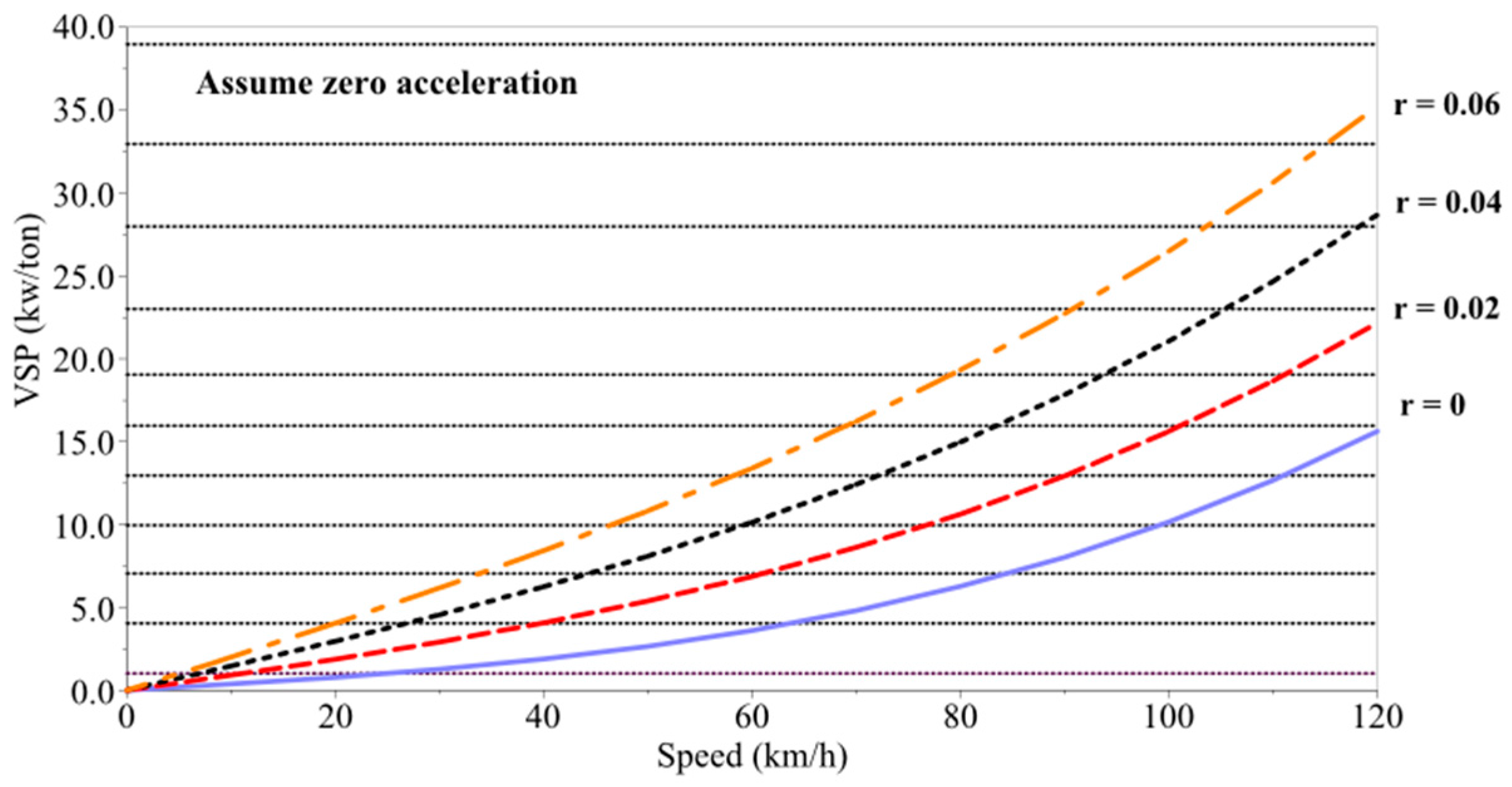
Note that a measure to quantify vehicle emissions has also been suggested. Vehicle-specific power (VSP) is defined as the instantaneous power per unit mass of the vehicle, which is subject to vehicle speed, acceleration, and road grade to estimate engine power demand while accounting for rolling resistance and aerodynamic drag. Assuming zero acceleration to simplify the sensitivity analysis, road grade was varied from 0 to 6%. Figure 1 shows the sensitivity of VSP and emissions to road grade and speed [20].

This paper aims to solve the GVRP with the objective of minimizing GHG emissions, considering various realistic factors including three-dimensional customer locations, gravity, vehicle speed, vehicle operating time, vehicle capacity, rolling resistance, air density, road grade, and inertia. The driving duration has been discretized to remove integral operators in calculation without loss of generality. The proposed formulation is a nonlinear mixed integer programming model with vehicle speeds, vehicle weights, road grades, and vehicle routes as decision variables. Therefore, the proposed formulation cannot be solved using off-the-shelf solvers. Because the goal of this study is to provide insight into and understand the characteristics of GVRP, this study proposes a simple solution method (sweep algorithm for the initial solution and 2-opt local search algorithm for the improvements) to find vehicle routes of GVRP. Both the VRP and GVRP are complex problems considering vehicle capacity and vehicle operating times on top of the multiple traveling salesman problem (mTSP). That is, the VRP is a problem to find as many Hamiltonian circuits as vehicles, satisfying the vehicle capacity and vehicle operating time constraints. Because the 2-opt local search algorithm is used to find Hamiltonian circuits, the proposed formulation has been relaxed using Lagrangian multipliers for vehicle capacity and vehicle operating time constraints. In this way, the proposed Lagrangian-based solution method reduces the original objective function value of GHG emissions and the penalties for the violation of vehicle capacity and vehicle operating time constraints simultaneously.

For simplicity, this paper assumes that all vehicles are homogeneous, with identical capacity, vehicle capabilities, fuel types, and operating skills. Customers with their demands that cannot exceed the vehicle capacity without loss of generality are located randomly. Because the altitudes of customer locations need to be considered to determine the visiting sequence of a vehicle, three-dimensional coordinates are used to specify customer locations, instead of two-dimensional ones.

An important difference between the problem under consideration and traditional VRP is in the decision variables. In addition to the routes of vehicles, vehicle speed, vehicle weight, and road grades between two customer locations should also be determined.

The remainder of this paper is organized as follows. In Section 2, related work to estimate GHG emissions is introduced. In Section 3, the GVRP under consideration is described and formulated as a nonlinear mixed-integer programing model. A Lagrangian-relaxed formulation is then proposed with additional constraints in Section 4 to propose a simple solution method. In Section 5, the effectiveness and efficiency are demonstrated through computational experiments. The conclusions are given in Section 6.

2. Preliminaries on GHG Emissions

Various models to calculate the exact amount of GHG emissions have been proposed in recent years. These models can be categorized into macroscopic and mesoscopic models, as shown in

Table 1. GHG (greenhouse gas) emissions models.

Macroscopic Models	Mesoscopic Emission Models
MEET (Methodology for calculating transport emission and energy consumption) [8]	Mesoscopic fuel consumption and emission modeling [22]
HBEFA (Handbook Emission Factors for Road Transport) [23]	A dynamic mesoscopic emission model for signalized intersections [24]
EcoTransIT (Ecological Transport Information Tool for Worldwide Transports) [25]	GHG-emission models for assessing the eco-friendliness of road and rail freight transports [26]

. Macroscopic models estimate average emission rates using empirical experiment datasets and help to understand the factors that affect emissions. They capture relevant parameters (e.g., payload and speed) but neglect others (e.g., traffic conditions). Because they use experimental data from existing vehicles, they are not adjustable for individual variations of technological parameters. Hickman et al. [8] proposed an emission model to calculate energy usages and CO₂ emissions using experimental data from the MEET (methodology for calculating transport emission and energy consumption) project, which was conducted by the European Commission. Demir et al. [21] surveyed 13 macroscopic emission models that can be used to calculate and develop a national or regional emission inventory.

Mesoscopic models analyze fuel consumption and emissions using vehicle characteristics and traffic conditions. They combine micromodels to estimate the emissions more precisely. Their great advantage over macroscopic models is that they reflect the influence of traffic conditions and do not require extensive experiments. Recently, Kirschstein and Meisel [26] developed a mesoscopic model based on a simple, fundamental theory that GHG emissions are proportional to fuel consumption. They considered four forces affecting GHG emissions: rolling resistance, air density, road grade, and inertia. Their mesoscopic model has been employed and discretized as the objective function in the proposed mathematical model of this paper.

To derive the objective function in our proposed mathematical model, the base model of Kirschstein and Meisel [26] on well-to-wheel (WTW) emissions is summarized. The amount of GHG emissions (in grams) can be calculated by

$$\mathrm{GHG}=f\cdot \phi$$

(1)

where $f$ (in liters) indicates the amount of fossil fuel consumed by a vehicle within a transport process, and $\phi$ (in kilograms/liter) is the WTW emission coefficient, i.e., the amount of CO₂ emitted by burning one unit of fuel. The WTW emission coefficients $\phi$ for diesel and fuel oil are 3.15 and 3.41, respectively.

The amount of fuel $f$ can be estimated by

$$f=W\cdot \sigma \cdot \frac{1}{\epsilon }$$

(2)

where $W$ (in kWh) is the expected total energy for moving a vehicle, $\sigma$ (in liters/KWh) is the WTW energy coefficient, i.e., the quantity of fuel generating 1 kWh—and another dimensionless coefficient $\epsilon ={\epsilon }^e\cdot {\epsilon }^t$ is the WTW energy coefficient, representing the efficiency of the combustion engine (${\epsilon }^e$) and the powertrain (${\epsilon }^t$). $W$ can be estimated from the physical properties of the vehicle, the characteristics of the route, the expected driving speed, and the expected traffic conditions. Hence, GHG emissions can be calculated by

$$\mathrm{GHG}=\frac{W}{\epsilon }\cdot \sigma \cdot \phi ,$$

(3)

Because the parameters $\epsilon ,\sigma$ and $\phi$ are subject to the physical properties of vehicles and fuels, estimating $W$ is important. This energy is governed by physical rules in thermodynamics, which convert the chemical energy of the fuel into kinematic energy of the vehicle. Ross [27] and Scora and Barth [28] calculated $W$ by determining the power required to overcome resistance from four main forces: rolling resistance, air drag, grade and inertia.

The power to overcome rolling resistance is calculated by

$$P^{roll}\left(m,v\right)=c^{roll}\cdot g\cdot m\cdot v$$

(4)

where $c^{roll}$ denotes the rolling resistance coefficient, $g$ is the gravitational acceleration, i.e., $g$ = 9.81 m/s², $m$ (in tons) is the total vehicle weight, and $v$ (in meters/second) represents the vehicle speed.

The power to overcome air resistance is calculated by

$$P^{air}\left(v\right)=\frac{1}{2000}\cdot c^{air}\cdot \rho \cdot A\cdot v^3$$

(5)

where $c^{air}$ denotes the drag coefficient, $\rho$ is the air density, i.e., $\rho$ = 1.2 kg/m³, and $A$ (in square meters) is the frontal surface area.

The power to overcome the road grade is calculated by

$$P^{grade}\left(m,v,\theta \right)=m\cdot g\cdot v\cdot r$$

(6)

where $r$ is the road grade in percent, i.e., r = $\tan \theta$, and $\theta$ is explained in relation to $r$ with the illustration in the following section.

The power to overcome inertia is calculated by

$$P^{inert}\left(m,v\right)=\frac{1}{2}\cdot m^{inert}\cdot \alpha \cdot v$$

(7)

where $\alpha$ denotes the acceleration, and $m^{inert}$ is the inertial mass in tons.

The total energy consumption can be obtained by integrating the total power level over the trip duration as

$$W={{\displaystyle \int }}_{t=t_1}^{t_2}P\left(v\left(t\right),\alpha \left(t\right),r\left(t\right),m\right)dt$$

(8)

where $P\left(v\left(t\right),\alpha \left(t\right),r\left(t\right),m\right)=P^{roll}\left(m,v\right)+P^{air}\left(v\right)+P^{grade}\left(m,v,\theta \right)+P^{inert}(m,v)$, and time indices $t_1$ and $t_2$ are the start and end of the trip, respectively. In this paper, we are interested in mass $m$, speed $v$, and road grade $r$, whereas physical and technical parameters such as $c^{roll}$, $c^{air}$, $\rho$, $A$, $m^{inert}$, and $\alpha$ could be considered as variables depending on the route a vehicle takes. Therefore, these physical and technical parameters are assumed to be fixed in our formulation.

3. Problem Description and Mathematical Formulations

The GVRP under consideration in this paper is defined as a VRP, in which the amount of GHG emissions needs to be minimized, so that customers with demands at different geographical locations and different altitudes are visited by a vehicle whose GHG emissions are subject to vehicle weights, vehicle speeds, road grades, and gravity.

The GVRP can be represented as a three-dimensional graph, where the vertices are in the three-dimensional space, i.e., $(x_i,y_i,z_i)$ for vertex i, and the arcs connect pairs of vertices. In this paper, $G=\left(V,A\right)$ represents a complete and symmetric graph, where $V=\left\{0,\dots ,n\right\}$ denotes vertices 1, 2, …, n for n customers and 0 for the depot, and $A$ is the arc set whose elements connect all pairs of vertices. 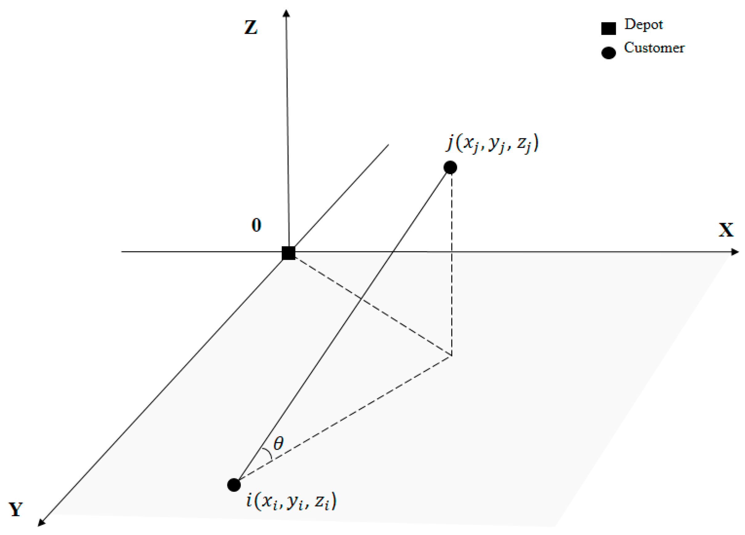Figure 2 exemplifies a three-dimensional space with a depot at the origin and two customers i and j.

Vertex i corresponds to a customer with a nonnegative demand $D_i\le c$, where $c$ is the vehicle capacity. A nonnegative Euclidean distance $d_{ij}$ between vertices i and j is $\sqrt[2]{{\left(x_i-x_j\right)}^2+{\left(y_i-y_j\right)}^2+{\left(z_i-z_j\right)}^2}$. For simplicity, we assume symmetricity, i.e., $d_{ij}=d_{ji}$. Angle $\theta$ can be calculated by $\arcsin \frac{\left|z_i-z_j\right|}{d_{ij}}$. The road grade $r_{ij}$ is the ratio of the elevation difference to the horizontal distance between locations i and j, i.e., $r_{ij}=\frac{\left|z_i-z_j\right|}{\sqrt[2]{{\left(x_i-x_j\right)}^2+{\left(y_i-y_j\right)}^2}}$. Because the power to overcome the road grade is considered only when θ > 0, the road grade can be expressed as $r_{ij}$ = tan θ.

It is assumed that $K$ identical vehicles are available at the depot. $T$ denotes the maximum vehicle operating time for all vehicles. It is also assumed that all customers can be visited only once by a single vehicle that starts from and returns to the depot. $v_{ij}$ is the average vehicle speed from vertices $i$ and $j$ with an upper bound $(v_{max})$ and lower bound $(v_{min})$. The total demand of customers on any vehicle’s route cannot exceed the vehicle capacity.

The altitudes of customer locations are important parameters in calculating the total GHG emissions due to the gravity and the different amounts of loads that vehicles carry on the different segments of the route, depending on the visiting sequences. The vehicle speed is another important control parameter because it can be controlled to reduce GHG emissions or add additional customers to existing routes.

The assumptions of the model are itemized as follows:

(1)

Vehicles are homogenous; i.e., each vehicle has identical loading capacity, maximum speed, maximum operating time, and empty vehicle weight.

(2)

The total customer demand on any vehicle’s route cannot exceed the vehicle capacity.

(3)

Each customer has a nonnegative demand that must be within the maximum vehicle capacity.

(4)

Each vehicle starts from the depot and returns to the depot.

(5)

Each customer can be visited only once by a single vehicle.

The objective of the proposed GVRP is to minimize GHG emissions under constraints of the traditional VRP, considering the altitudes of customer locations, vehicle weight changes, and vehicle speed.

A nonlinear mixed integer programming formulation for the GVRP under consideration is presented in the following with a list of input parameters and decision variables.

Input parameters:

• N: Number of customer.
• K: Number of vehicles at depot.
• D_i: Demand of customer i.
• c: Vehicle capacity.
• T: Maximum vehicle operating time.
• d_ij: Euclidean distance from customers i to j.
• r_ij: Road grade between customers i and j.

Decision variables:

• $x_{ijk}$: $\{\begin{array}{l}1,\mathrm{if}\left(i,j\right)\mathrm{is}\mathrm{on}\mathrm{the}\mathrm{route}\mathrm{of}\mathrm{vehicle}k.\\ 0,\mathrm{otherwise}.\end{array}$
• $m_{ij}$: Vehicle weight during the trip between customers $i$ and j.
• $v_{ij}$: Average vehicle speed during the trip between customers $i$ and j.
• $t_i$: Time point when a vehicle visits customer i.

A mathematical formulation of the GVRP under consideration is as follows. Note that the integral part of the GHG emission calculation in Equation (8) has been discretized by assuming that the driver maintains the vehicle speed at $v_{ij}$ without acceleration, i.e., ${\alpha }_{ij}$ = 0; the road grade $r_{ij}$ = tan θ is constant, as defined in Figure 2; and the vehicle weight, $m_{ij}$, is unchanged during the trip between locations i and j.

Minimize

$$Z={\sum }_{i=0}^N{\sum }_{j=0}^N{\sum }_{k=1}^K\frac{1}{\epsilon }\sigma \phi x_{ijk}P\left(v_{ij},{\alpha }_{ij},r_{ij},m_{ij}\right)\left(t_j-t_i\right)$$

(9)

Subject to

$${\sum }_{k=1}^K{\sum }_{j=1}^N{x}_{ijk}\le K,\mathrm{for}i=0$$

(10)

$${\sum }_{j=1}^N{x}_{0jk}\le 1,\mathrm{for}\forall k$$

(11)

$${\sum }_{i=1}^N{x}_{i0k}\le 1,\mathrm{for}\forall k$$

(12)

$${\sum }_{j=0}^N{x}_{ijk}-{\sum }_{j=0}^N{x}_{jik}=0,\mathrm{for}i=0,\dots ,N,\forall k$$

(13)

$${\sum }_{k=1}^K{\sum }_{j=0}^N{x}_{ijk}=1,\mathrm{for}i=1,\dots ,N$$

(14)

$${\sum }_{k=1}^K{\sum }_{i=0}^N{x}_{ijk}=1,\mathrm{for}j=1,\dots ,N$$

(15)

$${\sum }_{i=1}^N{D}_i\left({\sum }_{j=0}^N{x}_{jik}\right)\le c,\mathrm{for}\forall k$$

(16)

$${\sum }_{i=0}^N{\sum }_{j=0}^N{d}_{ij}{x}_{ijk}-v_{ij}T\le 0,\mathrm{for}\forall k$$

(17)

$$u_{ik}-u_{jk}+\left(N+1\right)x_{ijk}\le N,\mathrm{for}i\ne 0,j\ne 0,i\ne j,\forall k$$

(18)

$$x_{iik}=0,\mathrm{for}\forall i,\forall k$$

(19)

$$x_{ijk}\in \{0,1\},\mathrm{for}\forall i,\forall j,\forall k$$

(20)

$$u_{ik}\in ℝ,\mathrm{for}\forall i,\forall k$$

(21)

Objective Function (9) minimizes the total GHG emissions by $K$ vehicles. Note that $x_{ijk}$, $v_{ij}$, $r_{ij}$, $m_{ij},t_i$, and $t_j$ are variables determined by selecting a set of vehicle routes. Constraint (10) specifies the maximum number of vehicles available. Constraints (11) and (12) ensure that each vehicle which departs from the depot must return. Constraint (13) indicates the flow conservation. Constraints (14) and (15) ensure that each customer is visited only once by a single vehicle. Constraint (16) states that each vehicle carries no more than the vehicle capacity. By Constraint (17), each vehicle’s duration of trip must be less than the maximum vehicle operating time. Note that the visit to customers takes no time. Constraint (18) is a well-known Miller-Tucker-Zemlin subtour elimination constraint [29], where $u_{ik}$ and $u_{jk}$ are auxiliary variables. Constraint (19) prevents a vehicle from leaving and returning to the same customer location. Finally, binary integrity is specified by Constraint (20). Constraint (21) defines the auxiliary variables in Constraint (18).

As mentioned in Section 1, the above formulation cannot be solved using software for convex programming. In addition, the VRP is an NP-hard problem. It can be conjectured that the proposed formulation is very difficult to solve. Therefore, we have relaxed the feasible region of this formulation to convert VRP to mTSP, using Lagrangian relaxation.

Lagrangian relaxation is a technique well suited for problems in which the constraints are difficult to solve. The basic idea is to remove the “hard” constraints and put them into the objective function, assigned with the Lagrangian multipliers [30]. Thus, the problem becomes how to find the “hard” constraints and calculate the Lagrangian multipliers. In our formulation, the “hard” constraints are Constraints (16) and (17). If those constraints are lifted into the objective function, the Lagrangian relaxed formulation for GVRP can be transformed as follows.

Minimize

$$\begin{gathered} Z^{LR}={\displaystyle \sum }_{i=0}^N{\displaystyle \sum }_{j=0}^N{\displaystyle \sum }_{k=1}^K\frac{1}{\epsilon }\sigma \phi x_{ijk}P\left(v_{ij},{\alpha }_{ij},r_{ij},m\right)\left(t_j-t_i\right)+{\displaystyle \sum }_{p=1}^K{\alpha }_p\left({\displaystyle \sum }_{i=0}^N{D}_i{\displaystyle \sum }_{j=0}^N{x}_{ijp}-c\right) \\ +{\displaystyle \sum }_{q=1}^K{\beta }_q\left({\displaystyle \sum }_{i=0}^N{{\displaystyle \sum }}_{j=0}^N{d}_{ij}{x}_{ijq}-v_{ij}T\right) \end{gathered}$$

(22)

Subject to Constraints (10)–(15) and (18)–(21)

$${\sum }_{i=1}^N{\sum }_{j=1}^N{D}_i{x}_{ijp}-{\sum }_{i=1}^N{\sum }_{j=1}^N{D}_i{x}_{ij\left(p+1\right)}\ge 0\mathrm{for}p=1,\cdots ,K-1$$

(23)

$$\begin{array}{l}{\sum }_{i=1}^N{\sum }_{j=1}^N(d_{ij}{x}_{ijq}-v_{ij}T)-\\ {\sum }_{i=1}^N{\sum }_{j=1}^N(d_{ij}{x}_{ijq+1}-v_{ij}T)\ge 0\end{array}\mathrm{for}q=1,\cdots ,K-1$$

(24)

In the above Lagrangian-relaxed formulation, the amount of violations in the hard constraints (Constraints (16) and (17)) is multiplied by their dual variables (Lagrangian multipliers) and included in the objective function. Since the original problem is relaxed, it is easier to solve and provides a lower bound of the optimum (in the case of the minimization problem). This relaxed problem has a feasible region of mTSP, and we propose a simple solution method to obtain good solutions of mTSP. Constraints (23) and (24) are included so that the proposed algorithm performs more efficiently. The purpose is explained in the following paragraph.

Given a set of routes to satisfy all customers’ demands, where there are P and Q routes violating the vehicle capacity and operating time constraints, respectively, we want to index the corresponding routes as p = 1, 2, …, P and q = 1, 2, …, Q in the order of violation amounts. Lagrangian multipliers ${\alpha }_p$ and ${\beta }_q$ are considered as penalties (per unit weight or per unit time violated) to routes p or q, which violate the vehicle capacity and operating time constraints, respectively. That is, ${\alpha }_1>{\alpha }_2>\cdots >{\alpha }_p$ and ${\beta }_1>{\beta }_2>\cdots >{\beta }_q$. By these constraints, the larger penalty is applied to the route with a more serious violation in terms of vehicle capacity or operating time constraints. If we are interested only in finding feasible solutions quickly, ${\alpha }_p$ and ${\beta }_q$ can be set to large numbers; however, these solutions might be far from the optimal solution. Because our purpose must be to find the feasible solutions closer to the optimal solution, we need to approach the feasible solutions by increasing ${\alpha }_p$ and ${\beta }_q$ gradually from small values.

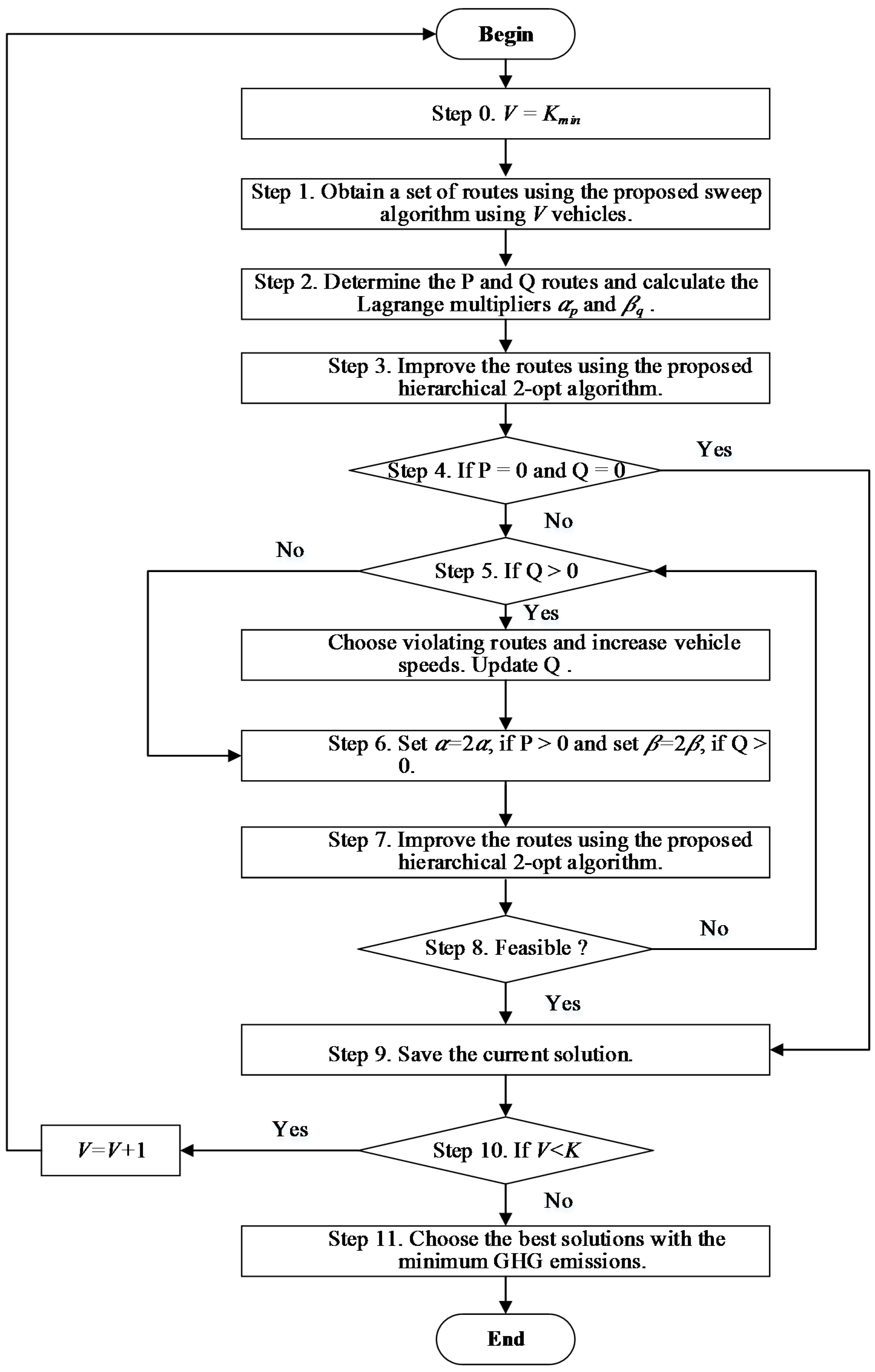
4. Proposed Solution Method

Because VRPs are NP-hard problems, many heuristic methods to find good solutions in a reasonable time have been proposed. The GVRP in this paper is more complicated since there are additional decision variables such as vehicle speeds, vehicle weights, and road grades, and there are nonlinear terms of order greater than 2 in the objective function.

The underlying approach is that the feasible region of the original GVRP is relaxed into the mTSP by Lagrangian relaxation, and then a sweep algorithm and a hierarchical 2-opt algorithm are used to obtain good solutions to the relaxed problem. The proposed solution method in this section minimizes GHG emissions and violation penalties simultaneously.

As initial solutions, it is almost impossible to obtain the feasible solutions to the original GVRP. We start from a simple solution, in which all customers are served by a certain number of vehicles even if there are violations in vehicle capacity or vehicle operating time. The minimum number of vehicles is defined as follows:

$$K_{min}=\lceil \frac{{\sum }_{i=1}^N{D}_i}{c}\rceil$$

(25)

The number of customers $Ng$ in each group is determined by

$$Ng=\lceil \frac{N}{U}\rceil$$

where $U\in \left\{K_{min},\dots ,K\right\}$ and $K_{min}\le K$.

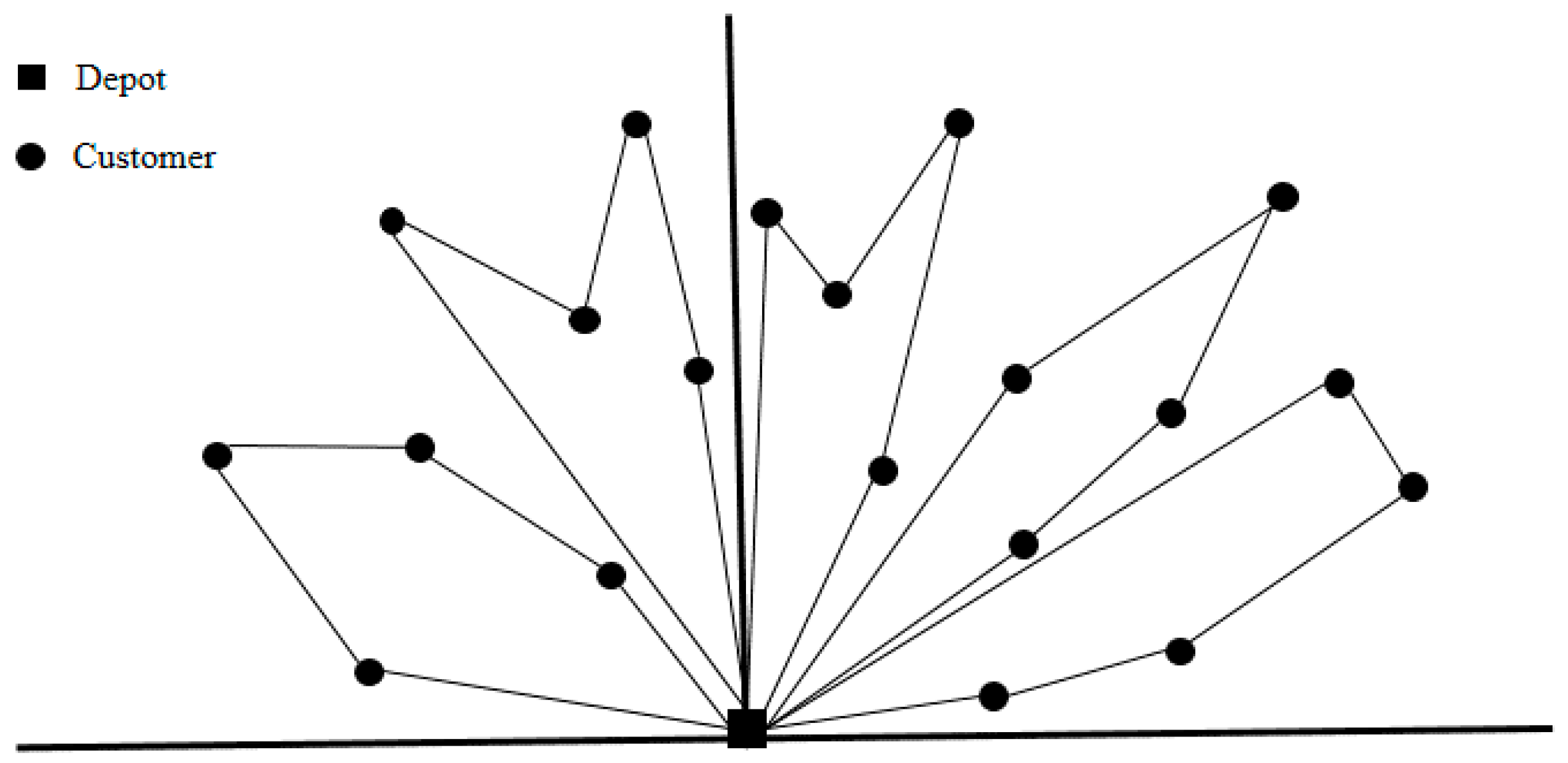
To initially obtain multiple Hamiltonian circuits as a feasible solution to mTSP, the sweep algorithm has been selected owing to its simplicity among many algorithms proposed in the past.

Gillett and Miller (1974) [31] introduced the sweep algorithm, which is one of the most well-known two-phase constructive methods to solve medium-scale and larger-scale capacitated vehicle routing problems (CVRPs) with load and distance constraints for each vehicle. It decomposes the CVRP by clustering geographically close customers into groups, such that each group is serviced by a single vehicle. To cluster customers in this paper, an identical number of customers is assigned into each group, considering the numbers of customers and available vehicles, instead of the customer demands and the vehicle capacity. A route is then created by connecting neighbors in angular proximity. When determining angular locations of customers, only x and y coordinates are considered. An example of the initial solution by the sweep algorithm is illustrated in Figure 3.

Because the demands of customers on each route and the driving times are not considered in the initial solution by the sweep algorithm, there are routes (or vehicles) where vehicle capacity and vehicle operating time constraints are violated. As mentioned previously, if there are P and Q routes violating the vehicle capacity and operating time constraints, respectively, we want to place them in the order of violation amounts and set ${\alpha }_1>{\alpha }_2>\cdots >{\alpha }_p$ and ${\beta }_1>{\beta }_2>\cdots >{\beta }_q$. Heuristically, the Lagrangian multiplier or penalty for violating the vehicle capacity, ${\alpha }_p$, is calculated in proportion to ${\alpha }_1$ in the ratio of violation amounts as follows:

$${\alpha }_p={\alpha }_1\times \frac{{\sum }_{i=1}^N{\sum }_{j=1}^N{D}_i{x}_{ijp}-c}{{\sum }_{i=1}^N{\sum }_{j=1}^N{D}_i{x}_{ij1}-c}$$

where ${\alpha }_1=\frac{\max \left(D_i\right)}{N\times \max \left(d_{ij}\right)}$.

Similarly, the Lagrangian multiplier or penalty for violation of the vehicle operating time, ${\beta }_q$, is calculated as follows:

$${\beta }_q={\beta }_1\times \frac{{\sum }_{i=1}^N{\sum }_{j=1}^N\frac{d_{ij}}{v_{ij}}{x}_{ijq}}{{\sum }_{i=1}^N{\sum }_{j=1}^N\frac{d_{ij}}{v_{ij}}{x}_{ij1}}$$

where ${\beta }_1=\frac{\max (\frac{d_{ij}}{v_{ij}})}{N\times \max \left(d_{ij}\right)}$.

These Lagrangian multipliers are used to evaluate the objective function of the Lagrangian-relaxed GVRP. A hierarchical 2-opt algorithm given in the following improves the routes to minimize Z^LR using these ${\alpha }_p$ and ${\beta }_q$.

The k-opt algorithm has been widely used in traveling salesman problems as a local search method [32]. The time complexity for k-opt is $O\left(n^k\right)$, where $n$ indicates the number of customers. The 2-opt algorithm is a special case of the k-opt algorithm, wherein each step, k arcs of the current tour are replaced by k arcs such that a smaller objective function is achieved.

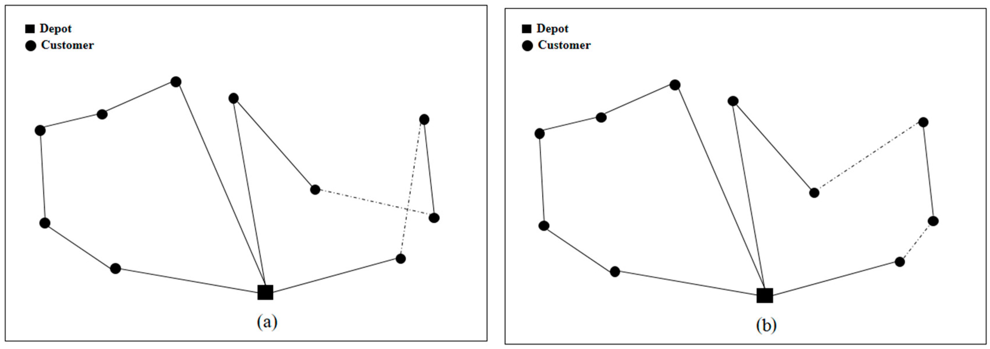
A hierarchical 2-opt algorithm has been proposed: inter-2-opt and intra-2-opt algorithms. The inter-2-opt algorithm between two routes removes an edge from each route and reconnects the remaining routes using two new edges as long as Z^LR is improved. Figure 4 shows two sets of possible routes. Assuming that Z^LR in Figure 4a is greater than Z^LR in Figure 4b, the dotted edges in Figure 4a are removed, and the dotted edges in Figure 4b are added to improve the routes.

The intra-2-opt algorithm within a route removes two edges and reconnects the remaining edges using two new edges as long as Z^LR is improved. Figure 5 shows two sets of possible routes. Assuming that Z^LR in Figure 5a is greater than Z^LR in Figure 5b, the dotted edges in Figure 5a are removed, and the dotted edges in Figure 5b are added to improve the routes.

The complete algorithm proposed in this paper has been summarized in the following and is illustrated in Figure 6.

• Lagrangian-based GVRP solution method

  Step 0

  V = K_min

  Step 1

  Obtain a set of routes using the proposed sweep algorithm using V vehicles.

  Step 2

  Determine P and Q routes that violate the vehicle capacity and operating time constraints, respectively, and calculate Lagrangian multipliers ${\alpha }_p$ and ${\beta }_q$.

  Step 3

  Improve the routes using the proposed hierarchical 2-opt algorithm.

  Step 4

  Test if P = 0 and Q = 0. If yes, go to Step 9.

  Step 5

  If Q > 0, choose the violating route, and increase the vehicle speed by setting $v_{ij}=v_{ij}+1$ in each road segment (i, j) of the route until the maximum vehicle speed in all segments of the routes is reached. Decrease Q by 1 whenever a route that violated the vehicle operating time constraint becomes feasible by increasing the vehicle speed.

  Step 6

  Set $\alpha =2\alpha$, if P > 0. Set $\beta =2\beta$, if Q > 0.

  Step 7

  Improve the routes using the proposed hierarchical 2-opt algorithm.

  Step 8

  Test the feasibility of the current routes. If yes, go to Step 9. Otherwise, update P and Q and go to Step 5.

  Step 9

  Save the current solution.

  Step 10

  Set $V=V+1$; go to Step 1 if $V<K$.

  Step 11

  Choose the best solution with minimal GHG emissions.

5. Computational Results

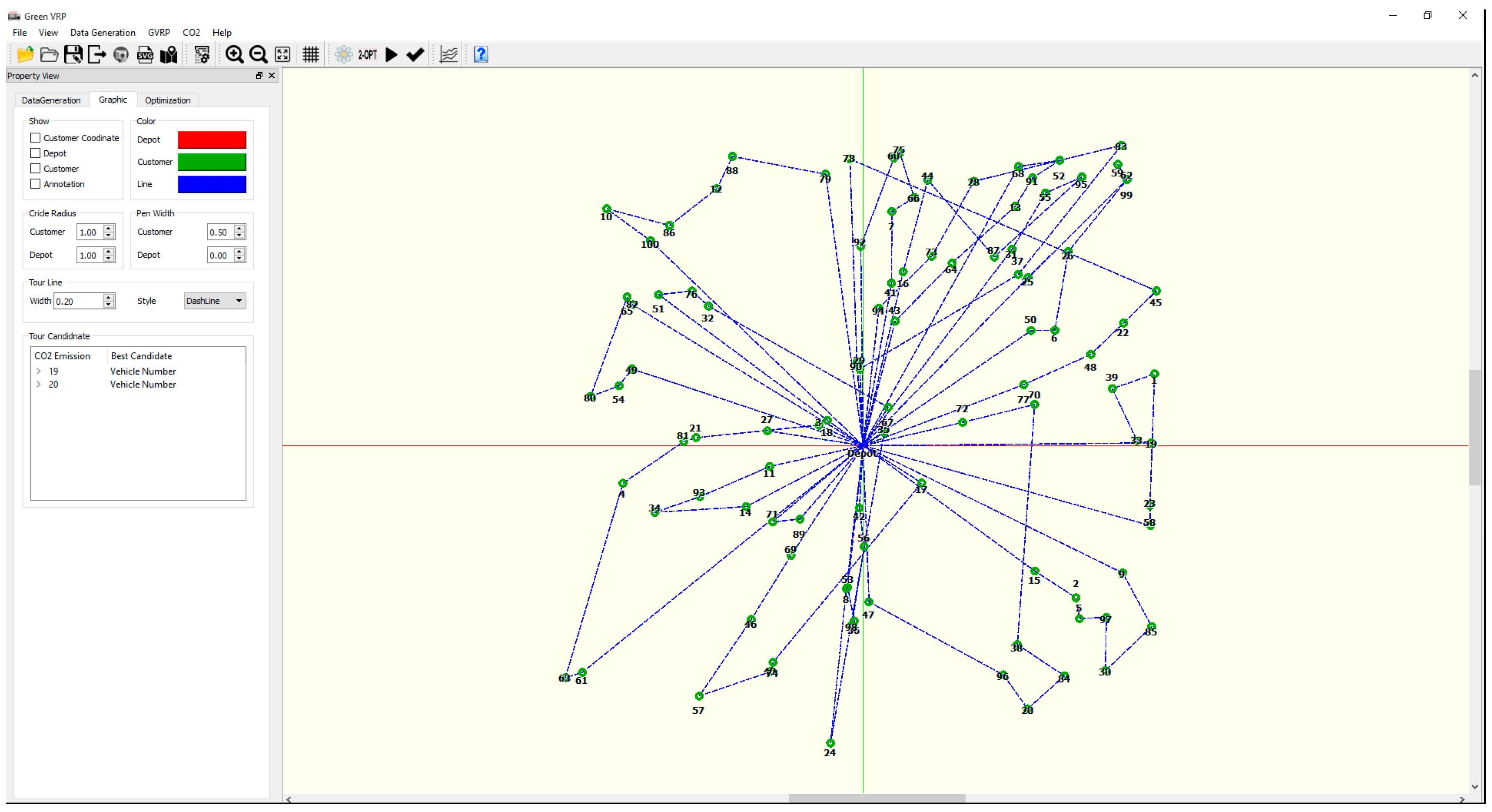
A complete solution method has been developed in the Visual C++ language with the QT library and implemented on a PC with an Intel Core i7-4792 CPU at 3.6 GHz and 16 GB of memory. The computation times in this section are recorded in seconds. The developed program demonstrates an example route visually as shown in Figure 7.

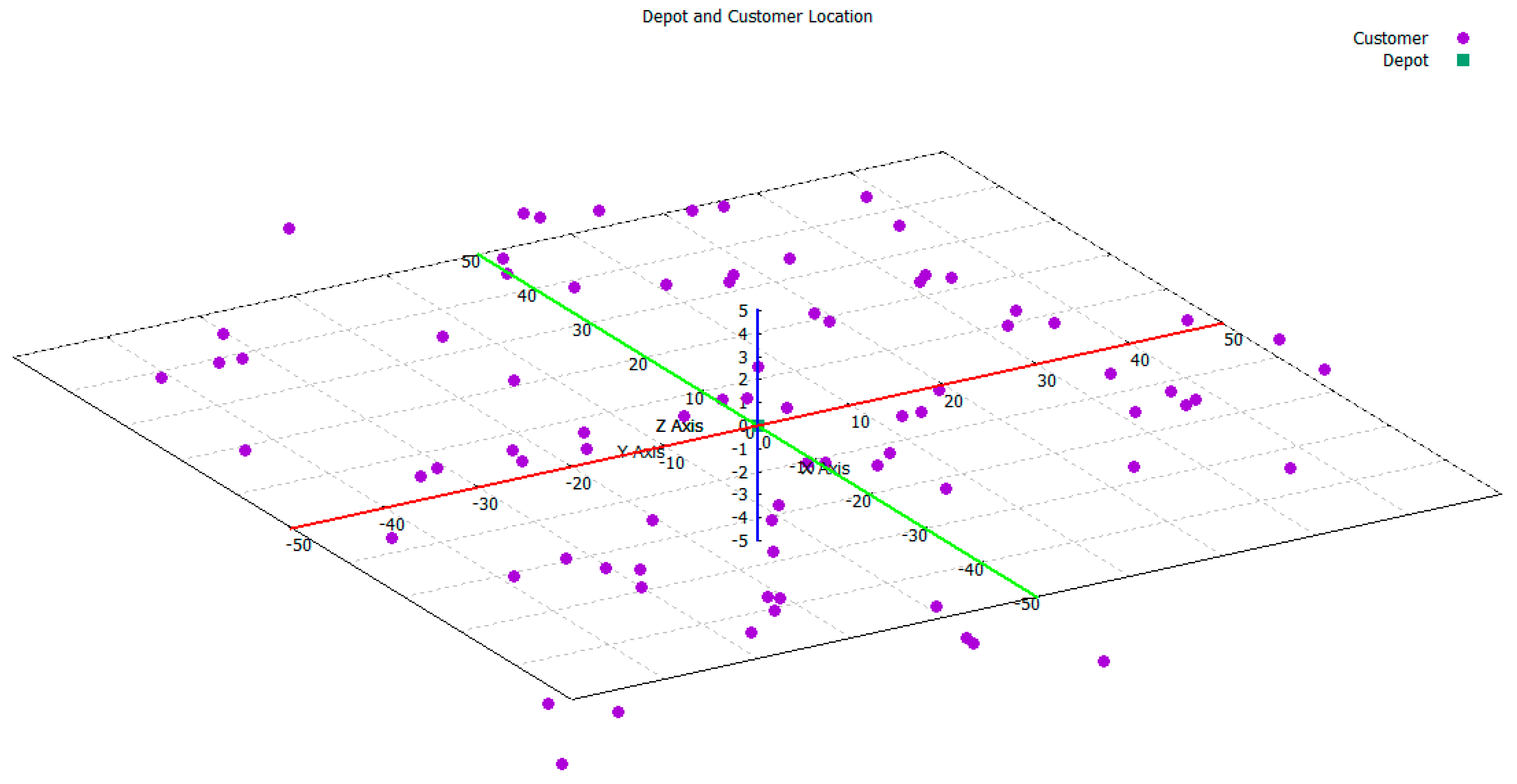
Experiments using various test problems have been run to assess the effectiveness and efficiency of the proposed solution method. The problem instances used in these experiments have been generated randomly as follows. The customers’ locations are generated three-dimensionally using uniform distributions with given ranges per axis, and the depot is always located at the origin (0, 0, 0). Figure 8 shows an example of a three-dimensional map for randomly generated customer locations using ranges [−50, 50] for the x- and y-axes and [−5, 5] for the z-axis. The customer demands are randomly generated by specifying the maximum demand per customer.

To demonstrate the computational significance of the proposed solution method, a small example with 9 customers is studied in this paragraph. The maximum demand per customer is set to 15. Customer locations are also randomly generated using ranges [−50, 50] for the x- and y-axes and [−5, 5] for the z-axis. The randomly generated data are given in

Table 2. Customer locations and their demands.

Customer	1	2	3	4	5	6	7	8	9
X	42.72	−27.13	2.97	−24.53	18.84	24.21	30.04	−29.18	49.41
Y	−19.72	−44.52	−34.54	6.48	−38.54	−46.05	27.37	−46.39	11.52
Z	−3.09	1.20	2.27	1.68	−2.05	4.47	2.16	−1.21	4.91
Demand	4	3	12	1	13	10	1	10	13

.

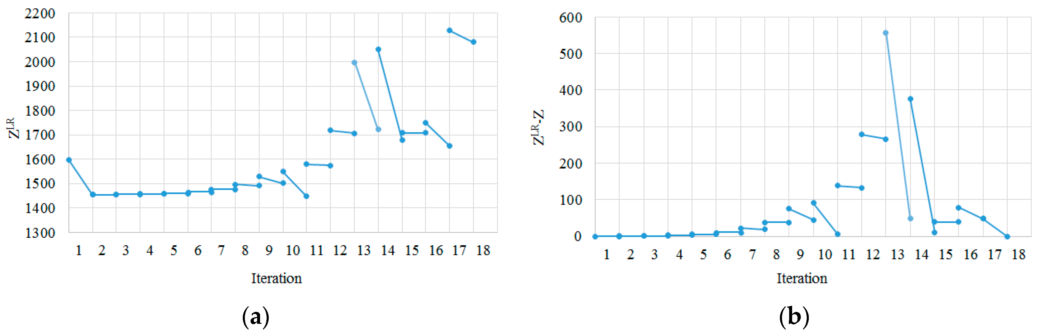
The number of available vehicles is 6, and their capacity is set to 15. The minimum and maximum vehicle speeds are 60 and 80 km/h, respectively. Thus, the minimum number of vehicles K_min = 5 according to Equation (25).

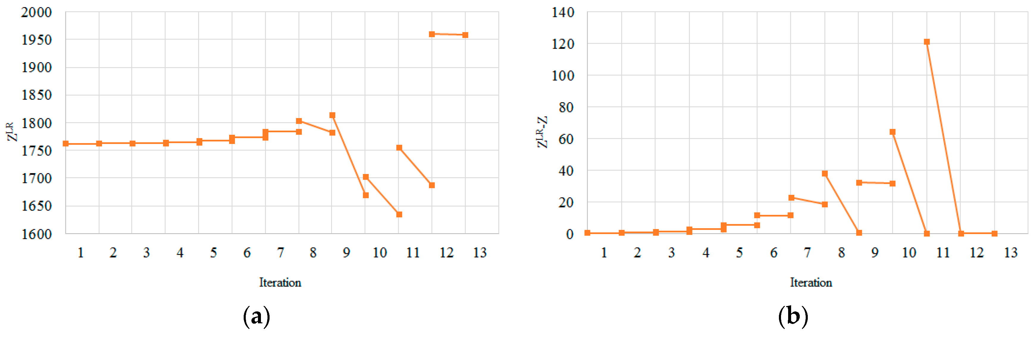
Figure 9 shows the Lagrangian-relaxed objective function values, Z^LR, and the penalties, Z − Z^LR, in each iteration when 5 vehicles are used. Figure 10 shows the same when 6 vehicles are used. In these figures, there is a line segment in each iteration, which shows the amount of changes in corresponding values during each iteration of the proposed solution method. On each vertical grid line, there are two values that represent the value at the end of the previous iteration and the other at the beginning of the next iteration. This is because the proposed solution method updates the violating constraints and Lagrangian multipliers ${\alpha }_p$ and ${\beta }_q$ in every iteration, and then the values of Z^LR or Z − Z^LR are re-evaluated. Since Lagrangian multipliers ${\alpha }_p$ and ${\beta }_q$ monotonically increase, the corresponding values at the beginning of the next iteration are always greater than the other. Note that some values are close and overlap in the figures.

In Figure 9a and Figure 10a, the feasible solutions for 5 and 6 vehicles are found by the penalty reaching 0 in iterations 18 and 13, respectively. As mentioned earlier, an important feature and advantage of the proposed solution method is to find the feasible solution close to the optimum because the GHG emissions and the penalty in the Lagrangian-relaxed objective function are minimized simultaneously, and Lagrangian multipliers ${\alpha }_p$ and ${\beta }_q$ are increased gradually from small values. It has been discovered that additional improvements for some test problems are possible by implementing additional steps of the proposed 2-opt algorithm on the feasible solutions found, but the gains are marginal. Since reporting the best possible solutions through additional steps is not the focus of this study, the details are omitted.

Table 3. Computational results for case study.

Number of Vehicles	Vehicle Routes	Vehicle Speeds between Locations (km/h)	GHG Emission (g)	Calculation Time (s)
5	0, 5, 0	60, 60	2080.36	0.323
	0, 3, 0	60, 60
	0, 1, 6, 0	74, 73, 73
	0, 4, 8, 2, 0	75, 75, 74, 74
	0, 9, 7, 0	65, 65, 64
6	0, 9, 7, 0	65, 65, 64	1959.36 *	0.207
	0, 5, 0	60, 60
	0, 4, 0	60, 60
	0, 8, 2, 0	62, 61, 61
	0, 1, 6, 0	74, 73, 73
	0, 3, 0	60, 60

* Best solution.

summarizes the computational results for this example. The best solution is obtained when 6 vehicles are used. As an example, a vehicle operation plan for the 5th vehicle is shaded in Table 3. This vehicle from the depot visits customers 1 and 6, and runs at a speed of 74, 73 and 73 km/h in trips (0, 1), (1, 6) and (6, 0), respectively.

Additional tests for problems of various sizes have been conducted.

Table 4. Small instance solution results.

Problem Size	Number of Customers	GHG Emission (g) *	Number of Vehicles Used	Fastest Speed (km/h)	Calculation Time (s)
Small	10	1761.73	7	67	0.507627
	15	1777.32	8	75	1.44431
	20	2253.71	10	68	2.77937
	25	3180.01	16	62	5.51869
	30	4164.73	18	62	14.1694
Medium	35	3741.96	17	64	22.2307
	45	4510.19	20	69	33.6993
	50	6463.4	28	63	95.2635
	60	8728.98	36	67	165.907
	70	10,644.9	42	63	292.479
Large	80	10,386.2	46	61	458.374
	90	13,323.8	55	73	710.432
	100	12,544.8	49	62	969.713
	110	8575.32	36	60	1130.80
	120	6431.91	23	69	1433.48

* Best solution.

shows the computational results for small, medium, and large problems in terms of the number of customers. The test problems are generated randomly using identical parameters to those explained for the above problem, which include customer locations, customer demands, vehicle capacity, vehicle operating time, and vehicle speed.

6. Conclusions

Concern and interest regarding GHG emissions have been emphasized more than ever. There have been many efforts to estimate the amount of GHG emissions in various approaches under different conditions. Those efforts need to be devoted to reducing GHG emissions.

In this study, the GVRP has been formulated as a nonlinear mixed integer programing model to minimize GHG emissions, considering various realistic factors including three-dimensional customer locations, gravity, vehicle speed, vehicle operating time, vehicle capacity, rolling resistance, air density, road grade, and inertia.

Studying the characteristics of the GVRP under consideration, the feasible regions of the proposed GVRP have been relaxed into mTSP by introducing Lagrangian multipliers to vehicle capacity and vehicle operating time constraints. A simple solution method using the sweep algorithm and 2-opt search algorithm has been proposed to simultaneously reduce the original objective function of GHG emissions and the penalties for the violation of constraints on vehicle capacity and vehicle operating time. The effectiveness and efficiency of the proposed solution method have been demonstrated by testing randomly generated problems.

Because vehicle speed is the most important factor affecting GHG emissions, vehicle speed, vehicle weight, and road grades between two customer locations are also optimized in addition to vehicle routes.

Finally, a user-friendly graphical user interface solver using the proposed solution method has been developed to solve the GVRP effectively. It will be further elaborated in future research.

Future studies should consider the following aspects: (1) adding fuel stations to extend the vehicle routes; (2) introducing fuel-efficient vehicles into the fleet; (3) allowing split deliveries; and (4) developing the solution method based on subgradients to solve the continuous nonlinear objective function. This study can be extended to production and distribution planning problem like Moon et al. [33].