A Hybrid Method for Short-Term Wind Speed Forecasting

Abstract
:1. Introduction
2. Methodology
2.1. EEMD
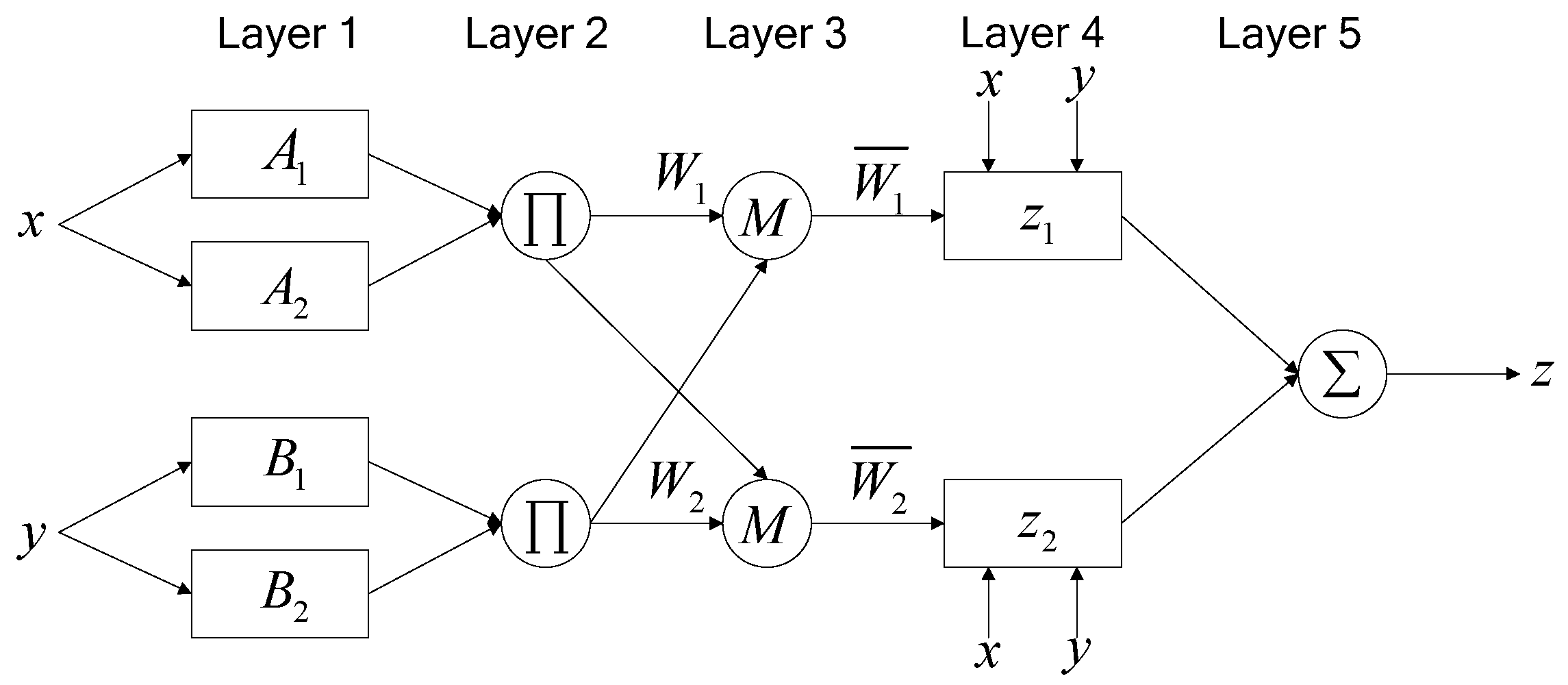
2.2. ANFIS
2.3. SARIMA
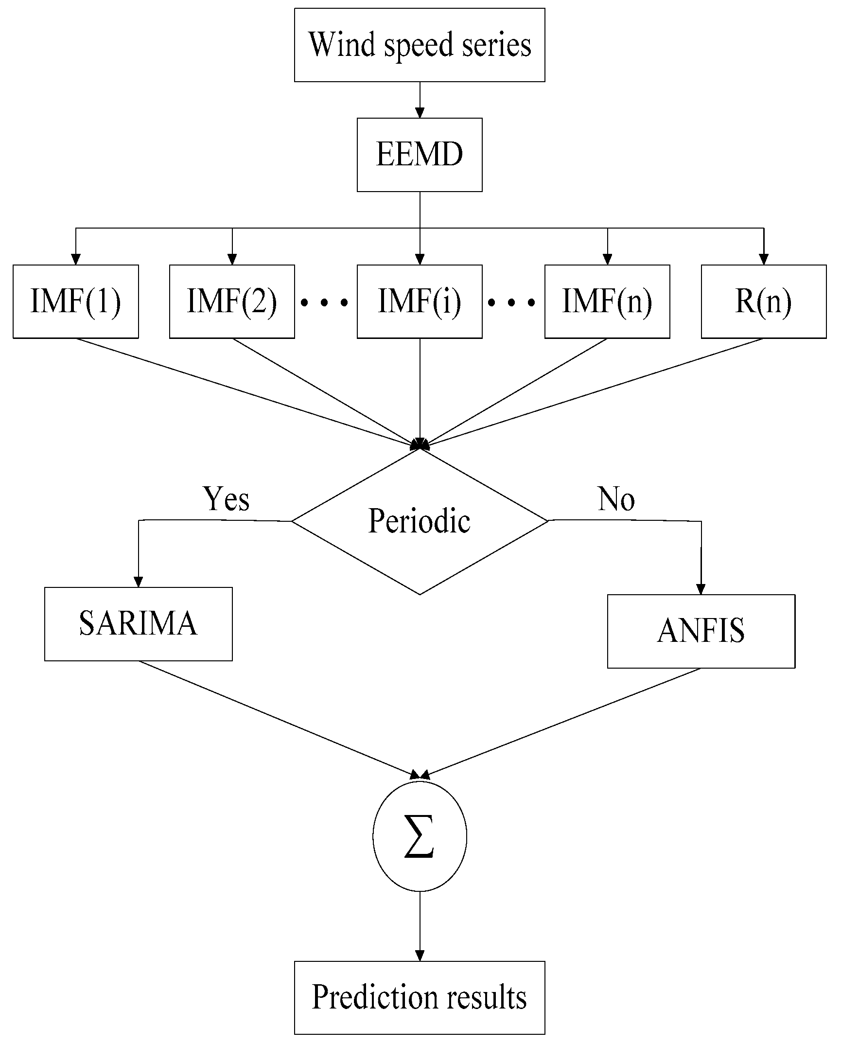
3. The Proposed Method
4. Numerical Results
4.1. Data Source
4.2. Case Studies
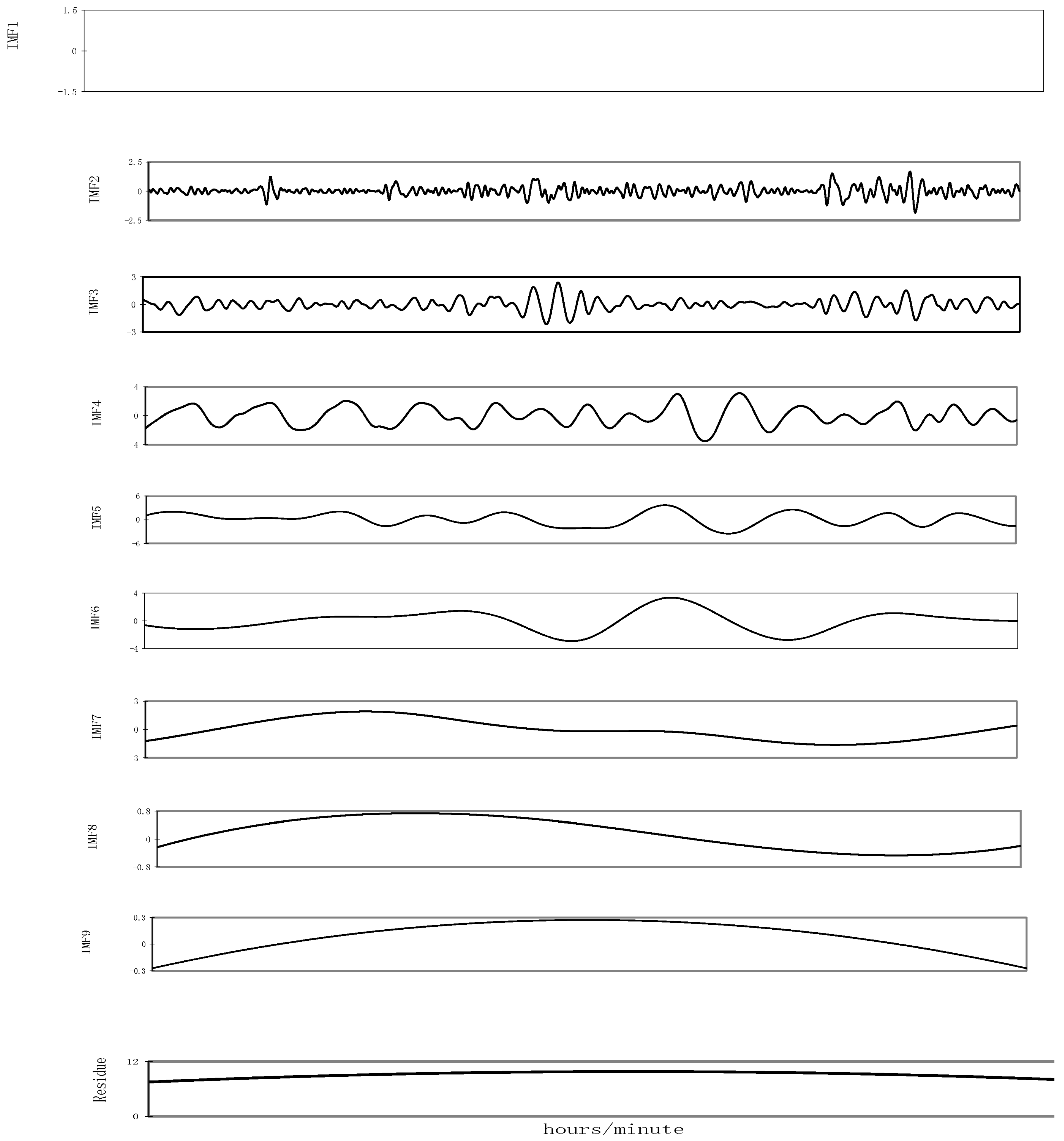
4.2.1. Wind Speed Series Decomposition.
4.2.2. Sub-Series Forecasting
4.3. Comparisons of ANFIS, SARIMA and the Proposed Method
4.3.1. Prediction Results for 24 h
4.3.2. Prediction Results for 3, 6 and 12 h
5. Conclusions
Acknowledgments
Author Contributions
Conflicts of Interest
References
- Erdem, E.; Shi, J. ARMA based approaches for forecasting the tuple of wind speed and direction. Appl. Energy 2011, 88, 1405–1414. [Google Scholar] [CrossRef]
- Liu, H.P.; Shi, J.; Erdem, E. Prediction of wind speed time series using modified Taylor Kriging method. Energy 2010, 35, 4870–4879. [Google Scholar] [CrossRef]
- Watson, S.J.; Landberg, L.; Halliday, J.A. Application of wind speed forecasting to the integration of wind energy into a large scale power system. IEE Proc. Gener. Transm. Distrib. 1994, 141, 357–362. [Google Scholar] [CrossRef]
- Landberg, L. Short-term prediction of the power production from wind farms. J. Wind Eng. Ind. Aerodyn. 1999, 80, 207–220. [Google Scholar] [CrossRef]
- Negnevitsky, M.; Johnson, P.; Santoso, S. Short term wind power forecasting using hybrid intelligent systems. In Proceedings of the IEEE Power Engineering General Meeting, Chicago, IL, USA, 24–28 June 2007; pp. 1–4. [Google Scholar]
- Alexiadis, M.C.; Dokopoulos, P.S.; Sahsamanoglou, H.S.; Manousaridis, I.M. Short term forecasting of wind speed and related electrical power. Sol. Energy 1998, 63, 61–68. [Google Scholar] [CrossRef]
- Damousis, I.G.; Alexiadis, M.C.; Theocharis, J.B.; Dokopoulos, P.S. A fuzzy model for wind speed prediction and power generation in wind parks using spatial correlation. IEEE Trans. Energy Convers. 2004, 19, 352–361. [Google Scholar] [CrossRef]
- Barbounis, T.G.; Theocharis, J.B. A locally recurrent fuzzy neural network with application to the wind speed prediction using spatial correlation. Neurocomputing 2007, 70, 1525–1542. [Google Scholar] [CrossRef]
- Beccali, M.; Girrincione, G.; Marvuglia, A.; Serporta, C. Estimation of wind velocity over a complex terrain using the generalized mapping regressor. Appl. Energy 2010, 87, 884–893. [Google Scholar] [CrossRef]
- Brown, B.G.; Katz, R.W.; Murphy, A.H. Time series models to simulate and forecast wind speed and power. J. Clim. Appl. Meteorol. 1984, 23, 1184–1195. [Google Scholar] [CrossRef]
- Lalarukh, K.; Yasmin, Z.J. Time series models to simulate and forecast hourly averaged wind speed in Quetta, Pakistan. Sol. Energy 1997, 61, 23–32. [Google Scholar]
- Poggi, P.; Muselli, M.; Notton, G.; Cristofari, C.; Louche, A. Forecasting and simulating wind speed in Corsica by using an autoregressive model. Energy Convers. Manag. 2003, 44, 3177–3196. [Google Scholar] [CrossRef]
- Torres, J.L.; García, A.; De Blas, M.; De Francisco, A. Forecast of hourly average wind speed with ARMA models in Navarre. Sol. Energy 2005, 79, 65–77. [Google Scholar] [CrossRef]
- Kavasseri, R.G.; Seetharaman, K. Day-ahead wind speed forecasting using f-ARIMA models. Renew. Energy 2009, 34, 1388–1393. [Google Scholar] [CrossRef]
- Mohandes, M.; Halawani, T.; Rehman, S.; Hussain, A.A. Support vector machines for wind speed prediction. Renew. Energy 2004, 29, 939–947. [Google Scholar] [CrossRef]
- Bilgili, M.; Sahin, B.; Yasar, A. Application of artificial neural networks for the wind speed prediction of target station using reference stations data. Renew. Energy 2007, 32, 2350–2360. [Google Scholar] [CrossRef]
- Mabel, M.C.; Fernandez, E. Analysis of wind power generation and prediction using ANN: A case study. Renew. Energy 2008, 33, 986–992. [Google Scholar] [CrossRef]
- Cadenas, E.; Rivera, W. Short term wind speed forecasting in La Venta, Oaxaca, México, using artificial neural networks. Renew. Energy 2009, 34, 274–278. [Google Scholar] [CrossRef]
- Abdel-Aal, R.; Elhadidy, M.; Shaahid, S. Modeling and forecasting the mean hourly wind speed time series using GMDH-based abductive networks. Renew. Energy 2009, 34, 1686–1699. [Google Scholar] [CrossRef]
- Gong, L.; Shi, J. On comparing three artificial neural networks for wind speed forecasting. Appl. Energy 2010, 87, 2313–2320. [Google Scholar]
- Thiaw, L.; Sow, G.; Fall, S.S.; Kasse, M.; Sylla, E.; Thioye, S. A neural network based approach for wind resource and wind generators production assessment. Appl. Energy 2010, 87, 1744–1748. [Google Scholar] [CrossRef]
- Jung, J.; Broadwater, R.P. Current status and future advances for wind speed and power forecasting. Renew. Sustain. Energy Rev. 2014, 31, 762–777. [Google Scholar] [CrossRef]
- Ma, L.; Luan, S.Y.; Jiang, C.W.; Liu, H.L.; Zhang, Y. A review on the forecasting of wind speed and generated power. Renew. Sustain. Energy Rev. 2009, 13, 915–920. [Google Scholar]
- Chen, T.L.; Cheng, C.H.; Teoh, H.J. High-order fuzzy time-series based on multi-period adaptation model for forecasting stock markets. Physica A 2008, 387, 876–888. [Google Scholar] [CrossRef]
- Rodriguez, C.P.; Anders, G.J. Energy price forecasting in the Ontario competitive power system market. IEEE Trans. Power Syst. 2004, 19, 366–374. [Google Scholar] [CrossRef]
- Zhang, Y.; Zhou, Q.; Sun, C.X.; Lei, S.L.; Liu, Y.M.; Song, Y. RBF neural network and ANFIS-based short-term load forecasting approach in real-time price environment. IEEE Trans. Power Syst. 2008, 23, 853–858. [Google Scholar] [CrossRef]
- Guo, Z.H.; Zhao, J.; Zhang, W.Y.; Wang, J.Z. A corrected hybrid approach for wind speed prediction in Hexi Corridor of China. Energy 2011, 36, 1668–1679. [Google Scholar] [CrossRef]
- Palm, F.C.; Zellner, A. To combine or not to combine? Issues of combining forecasts. Int. J. Forecast. 1992, 11, 687–701. [Google Scholar] [CrossRef]
- Lei, Y.G.; He, Z.J.; Zi, Y.Y. Application of the EEMD method to rotor fault diagnosis of rotating machinery. Mech. Syst. Sig. Process. 2009, 23, 1327–1338. [Google Scholar] [CrossRef]
- Wu, Z.; Huang, N. Ensemble empirical mode decomposition: a noise assisted data analysis method. Adv. Adapt. Data Anal. 2009, 1, 1–41. [Google Scholar] [CrossRef]
- Jang, J.S.R. ANFIS: Adaptive-Network-Based Fuzzy Inference System. IEEE Trans. Syst. Man Cybern. 1993, 23, 665–685. [Google Scholar] [CrossRef]
- Box, G.E.P.; Jenkins, G.M. Time Series Analysis: Forecasting and Control; Holden Day: San Francisco, CA, USA, 1976. [Google Scholar]


| Sites | Mean (m/s) | SD (m/s) | Min.Vel (m/s) | Max.Vel (m/s) |
|---|---|---|---|---|
| Site 1 | 9.26 | 3.84 | 0.18 | 28.21 |
| Site 2 | 9.05 | 4.05 | 0.19 | 30.73 |
| Forecast Horizon | Error | ANFIS | SARIMA | Proposed Method |
|---|---|---|---|---|
| 24 h 28 February 2006 | MAE | 0.15 | 0.14 | 0.05 |
| RMSE | 0.17 | 0.18 | 0.06 | |
| MAPE (%) | 1.87 | 1.83 | 0.66 | |
| 24 h 31 May 2006 | MAE | 0.23 | 0.30 | 0.13 |
| RMSE | 0.34 | 0.47 | 0.21 | |
| MAPE (%) | 3.98 | 5.06 | 2.39 | |
| 24 h 31 August 2006 | MAE | 0.19 | 0.42 | 0.11 |
| RMSE | 0.30 | 0.82 | 0.18 | |
| MAPE (%) | 1.44 | 2.92 | 0.83 | |
| 24 h 30 November 2006 | MAE | 0.14 | 0.15 | 0.08 |
| RMSE | 0.18 | 0.21 | 0.11 | |
| MAPE (%) | 1.17 | 1.30 | 0.67 |
| Forecast Horizon | Error | ANFIS | SARIMA | Proposed Method |
|---|---|---|---|---|
| 24 h 28 February 2006 | MAE | 0.18 | 0.20 | 0.07 |
| RMSE | 0.23 | 0.30 | 0.09 | |
| MAPE (%) | 2.18 | 2.51 | 0.79 | |
| 24 h 31 May 2006 | MAE | 0.24 | 0.34 | 0.13 |
| RMSE | 0.37 | 0.47 | 0.19 | |
| MAPE (%) | 4.33 | 6.44 | 2.57 | |
| 24 h 31 August 2006 | MAE | 0.22 | 0.55 | 0.13 |
| RMSE | 0.36 | 1.19 | 0.26 | |
| MAPE (%) | 1.83 | 3.55 | 1.08 | |
| 24 h 30 November 2006 | MAE | 0.16 | 0.19 | 0.08 |
| RMSE | 0.21 | 0.26 | 0.11 | |
| MAPE (%) | 1.40 | 1.56 | 0.68 |
| Forecast Horizon | Error | ANFIS | SARIMA | Proposed Method |
|---|---|---|---|---|
| 3 h 28/02/2006 | MAE | 0.17 | 0.18 | 0.06 |
| RMSE | 0.22 | 0.23 | 0.08 | |
| MAPE (%) | 1.95 | 2.11 | 0.75 | |
| 6 h 31/05/2006 | MAE | 0.31 | 0.46 | 0.11 |
| RMSE | 0.42 | 0.57 | 0.32 | |
| MAPE (%) | 4.52 | 6.32 | 2.45 | |
| 12 h 31/08/2006 | MAE | 0.32 | 0.51 | 0.23 |
| RMSE | 0.54 | 0.98 | 0.31 | |
| MAPE (%) | 1.44 | 3.31 | 0.94 | |
| Average | MAE | 0.26 | 0.38 | 0.13 |
| RMSE | 0.39 | 0.59 | 0.23 | |
| MAPE (%) | 2.63 | 3.91 | 1.38 |
| Forecast Horizon | Error | ANFIS | SARIMA | Proposed Method |
|---|---|---|---|---|
| 3 h 28/02/2006 | MAE | 0.29 | 0.34 | 0.12 |
| RMSE | 0.35 | 0.41 | 0.14 | |
| MAPE (%) | 3.21 | 3.12 | 0.87 | |
| 6 h 31/05/2006 | MAE | 0.38 | 0.54 | 0.18 |
| RMSE | 0.46 | 0.66 | 0.23 | |
| MAPE (%) | 5.57 | 7.02 | 3.12 | |
| 12 h 31/08/2006 | MAE | 0.44 | 0.69 | 0.21 |
| RMSE | 0.51 | 2.08 | 0.38 | |
| MAPE (%) | 2.49 | 4.01 | 1.77 | |
| Average | MAE | 0.37 | 0.52 | 0.17 |
| RMSE | 0.44 | 1.05 | 0.25 | |
| MAPE (%) | 3.75 | 4.71 | 1.92 |
© 2017 by the authors. Licensee MDPI, Basel, Switzerland. This article is an open access article distributed under the terms and conditions of the Creative Commons Attribution (CC BY) license (http://creativecommons.org/licenses/by/4.0/).
Share and Cite
Zhang, J.; Wei, Y.; Tan, Z.-f.; Ke, W.; Tian, W. A Hybrid Method for Short-Term Wind Speed Forecasting. Sustainability 2017, 9, 596. https://doi.org/10.3390/su9040596
Zhang J, Wei Y, Tan Z-f, Ke W, Tian W. A Hybrid Method for Short-Term Wind Speed Forecasting. Sustainability. 2017; 9(4):596. https://doi.org/10.3390/su9040596
Chicago/Turabian StyleZhang, Jinliang, YiMing Wei, Zhong-fu Tan, Wang Ke, and Wei Tian. 2017. "A Hybrid Method for Short-Term Wind Speed Forecasting" Sustainability 9, no. 4: 596. https://doi.org/10.3390/su9040596
APA StyleZhang, J., Wei, Y., Tan, Z.-f., Ke, W., & Tian, W. (2017). A Hybrid Method for Short-Term Wind Speed Forecasting. Sustainability, 9(4), 596. https://doi.org/10.3390/su9040596