Impact Assessment of Pollutant Emissions in the Atmosphere from a Power Plant over a Complex Terrain and under Unsteady Winds

Abstract

The development of a natural gas-fired tri-generation power plant (520 MW Combined Cycle Gas Turbines + 58 MW Tri-generation) in the Republic of San Marino, a small independent country in Northern Italy, is under assessment. This work investigates the impact of atmospheric emissions of NO_x by the plant, under the Italian and European regulatory framework. The impact assessment was performed by the means of the Aria Industry package, including the 3D Lagrangian stochastic particle dispersion model SPRAY, the diagnostic meteorological model SWIFT, and the turbulence model SURFPRO (Aria Technologies, France, and Arianet, Italy). The Republic of San Marino is almost completely mountainous, 10 km west of the Adriatic Sea and affected by land-sea breeze circulation. SPRAY is suitable for simulations under non-homogenous and non-stationary conditions, over a complex topography. The emission scenario included both a worst-case meteorological condition and three 10-day periods representative of typical atmospheric conditions for 2014. The simulated NO_x concentrations were compared with the regulatory air quality limits. Notwithstanding the high emission rate, the simulation showed a spatially confined environmental impact, with only a single NO_x peak at ground where the plume hits the hillside of the Mount Titano (749 m a.s.l.), 5 km west of the future power plant.

1. Introduction

The United Nations Framework Convention on Climate Change (UNFCCC) set the ultimate objective to prevent hazardous anthropogenic interference with the climate system.

To meet this goal, the European Commission promotes and supports the reduction in energy consumption, the increase in energy efficiency, the increase in energy production from renewable sources and the reduction in greenhouse gas (GHG) emissions; these commitments were set out in the Directive 2009/29/EC [1], and commonly called European 20-20-20 targets.

To fulfill the purposes of the Directive 2009/29/EC, the European Commission planned preliminary actions, including the promotion of the “cogeneration” [2]. Combined heat and power (CHP) production, or cogeneration, implies that heat and electricity are produced simultaneously in a single process, coupling electricity production technologies with heat recovery equipment [3]. Cogeneration is one of the most promising means of using existing advanced technologies for sustainable energy production.

CHP helps to reduce the environmental impact of power generation, because its self-production of electric power reduces the needs of electricity supply from the electric energy network with respect to a traditional power plant. Therefore, the pollutant (mainly NO_x, SO_x, and PM₁₀) and GHG emissions due to conventional electricity generation, which impact on air quality both at local [4] and at global scale [5], are avoided. Estimates by the European Environmental Agency [6] of the avoided CO₂ emissions by the use of CHP led to the classification of cogeneration as a low carbon technology.

For these reasons, environmental policies support the diffusion of cogeneration plants: the share of electricity produced from CHP in the EU-27 is growing since 2008 [7]. Nevertheless, the atmospheric impact of a cogeneration plant must be assessed, and the ground-level concentration of emitted pollutants must be compared with the air quality regulatory limits. That impact depends on the plant emission performance and on the dispersion of its stack emissions in atmosphere, i.e., the meteorological conditions and the local landscape features may also be relevant.

Economic sustainability of CHP plants is strongly influenced by the environmental impact of their atmospheric emissions [8], and therefore, by the topographic setting of plant location. The stack emissions are a key factor in assessing the plant impact on local air quality, but basing this impact simply upon the exhaust mass flow rate of the pollutants and/or its annual atmospheric emissions would lead to partial and inaccurate results. A realistic simulation of pollutant dispersion is needed to properly assess the economic costs of atmospheric impact by the plant. Moreover, the availability of accurate and extended (both in time and space) pollutant concentration fields, having a suitable spatio-temporal resolution, reduces the uncertainty in estimates of population exposure to atmospheric pollution [9].

Several studies based the environmental impact by atmospheric emissions using only statistical models, e.g., Land Use Regression models in urban areas [10] or Geographically Weighted Regression models in larger domains [11]. This type of models fails in estimating the impact by future point emissions, contrarily to dispersion models. Atmospheric dispersion models represent another important tool for atmospheric impact assessment of the stack emissions of power plants. These models allow one to simulate the spatial distribution of pollutants, in order to forecast the impact of an emitting source on air quality, or to identify the contribution of different sources, and support policy strategies for air pollution control.

Very few studies in the literature combined both a statistical and a dispersion model [12], moreover, they generally use simplistic dispersion tools (e.g., Gaussian models), which are based on strong assumptions, and suitable only in rarely occurring conditions. The present study combines the use of a statistical and a dispersion modelling tool, and it is featured by a Lagrangian dispersion model, representing a novelty and providing improved concentration fields for reliable economic assessments of the plant and exposure studies.

The Directive 2008/50/EC [13] and Italian law (D.Lgs. 152 03/04/2006) allow the application of dispersion models for the assessment of air quality, and set the uncertainty which may be applied to a simulation result. The models available are many, featured by different degrees of complexity and different performances. Simulation results produced by different models may not be comparable during some specific atmospheric conditions, such as low winds [14] or local scale winds of breeze, and also over complex topography [15,16,17,18,19,20,21].

The development of a natural gas-fired tri-generation power plant (520 MW Combined Cycle Gas Turbines (CCGT) + 58 MW Tri-generation) in the Republic of San Marino, a small independent enclave placed in Northern Italy, is under evaluation. The power plant will have the largest efficiency among all existing plants over the Italian peninsula, it will completely fulfill the energy needs of San Marino, and it will also provide energy to Italy.

The project could benefit from existing and near infrastructures, as gas pipelines and electricity grids export energy to Italy. Moreover, the Italian regions south of San Marino would have a major advantage from the plant, because of the lower number of cogeneration units and the lower electricity production capacity in these areas [22]. The project includes the use of cogeneration in combination with heat-pump technology and plug-in vehicles as part of a renewable electric grid, in order to make San Marino a “smart” society [23], with a more robust energy infrastructure which might drive economic growth.

The present work investigates the provisional impact assessment of atmospheric emissions from the cogeneration plant stacks, which could be installed in the Republic of San Marino, in the framework of the regulatory limits put by Italian law (D.Lgs. 152 03/04/2006 and D.Lgs. 46 04/03/2014, implementation of Directive 2010/75/UE [24]). Both technical and socioeconomic aspects of that project have great relevance, yet the environmental implications must be evaluated. Among these, the air pollution caused by the plant emissions, which receive more attention by the population, directly affecting human health.

The study includes simulation results from a Lagrangian dispersion model of the power plant during a worst-case scenario, and three periods well representative of low, moderate, and large atmospheric dispersion conditions, respectively. Only NO_x and CO were simulated, being the two compounds having regulatory emission limits for this power plant; since the simulated concentrations of CO were largely lower than the regulatory limits, the simulation focused only on NO_x. Finally, a statistical analysis of concentration fields has been performed to assess the impact of atmospheric emissions on local air quality, and on exceedance of air quality regulatory limits.

2. The Cogeneration Plant

The cogeneration plant considered is the Mitsubishi MHPS GT Model M701F5 and H-25(42) Combined Cycle Gas Turbines (CCGT, 520 MW and 58 MW thermal power respectively) powered by methane gas. The features of the plant and the estimates of NO_x concentrations in the dry exhaust gas (based on 15% O₂) for both the CCGT plant units are reported in

Table 1. Power Plant features, as provided by the manufacturer.

Unit	Stack Height	Stack Inner Diameter	Exhaust Gas Flow	Exhaust Gas Temperature	Gas Exit Velocity	NOx
	m	m	Nm3 h−1	°C	m s−1	mg Nm−3
M701F5 CCGT	70	6.2	1,885,000	85	25	50
H-25(42) CCGT	70	2.7	290,000	85	20	50

(NOTE: personal communication).

Regulatory emission limits are set by the Italian law for combustion plants with nominal thermal power >50 MW, large combustion plants (D.Lgs. 152 03/04/2006, and D.Lgs. 46 04/03/2014, implementation of Directive 2010/75/UE [24]). Regarding to the new power plants, regulatory limits for Gas Turbines (CCGT included) supplied by methane gas are equal to 30 mg Nm⁻³ for NO_x and 100 mg Nm⁻³ for CO in dry exhaust gas (based on 15% O₂). However, for plants with efficiency greater than 35%, the law (D.Lgs. 46 04/03/2014) sets the emission limit for NO_x equal to 30 × η (35%), where η (%) is the efficiency of the plant. For the plant in project, whose efficiency η = 61% (as assured by the Manufacturer), the emission limit for NO_x results in 52 mg Nm⁻³.

3. The Investigation Domain

The Republic of San Marino (RSM) is an enclave in Italy, on the border between the regions of Emilia Romagna, with the provinces of Forlì-Cesena and Rimini, and Marche, with the province of Pesaro-Urbino, at about 10 km from the Adriatic Sea coast. The country covers an area of about 61.2 km². It has a Mediterranean climate with mild to cool winters and warm, sunny summers. The Republic of San Marino is affected by land-sea breeze superimposed to a mesoscale circulation. RSM topography is dominated by the Apennine mountain chain, resulting in it being almost completely mountainous (83% of its territory). The highest point in the country is the summit of Mount Titano (749 m a.s.l.), with the largest town of RSM, San Marino City (4128 inhabitants), that is cited at 625 m a.s.l. on the West side of Mount Titano. The power plant will be installed (as shown in Figure 1a) East of the San Marino City, close to the Italian border, at an elevation of about 120 m a.s.l.

4. Software and Datasets

The simulation of the dispersion of the pollutant emitted by the plant was performed by the software package ARIA INDUSTRY (Arianet srl, Milano, Italy & ARIA Tehcnologies Boulogne Billancourt, France), which includes the dispersion model SPRAY, the diagnostic wind field meteorological model SWIFT (former MINERVE [25,26,27,28]) and the turbulence model SURFPRO [29]. SPRAY is a Lagrangian stochastic model for the simulation of the dispersion of passive pollutants in a complex terrain and non-homogenous conditions, under calm and low wind events [14]. The model operates in non-stationary conditions by approximating temporal variations in successive stationary states. SPRAY gives highly reliable simulations of pollutant dispersion close to the release source point [30,31], and it is able to simulate deposition-decay phenomena. SPRAY supplies a three-dimensional concentration field, vertically subdivided into grid cells at different terrain-following layers, and vertically stretched to obtain higher resolution near the ground.

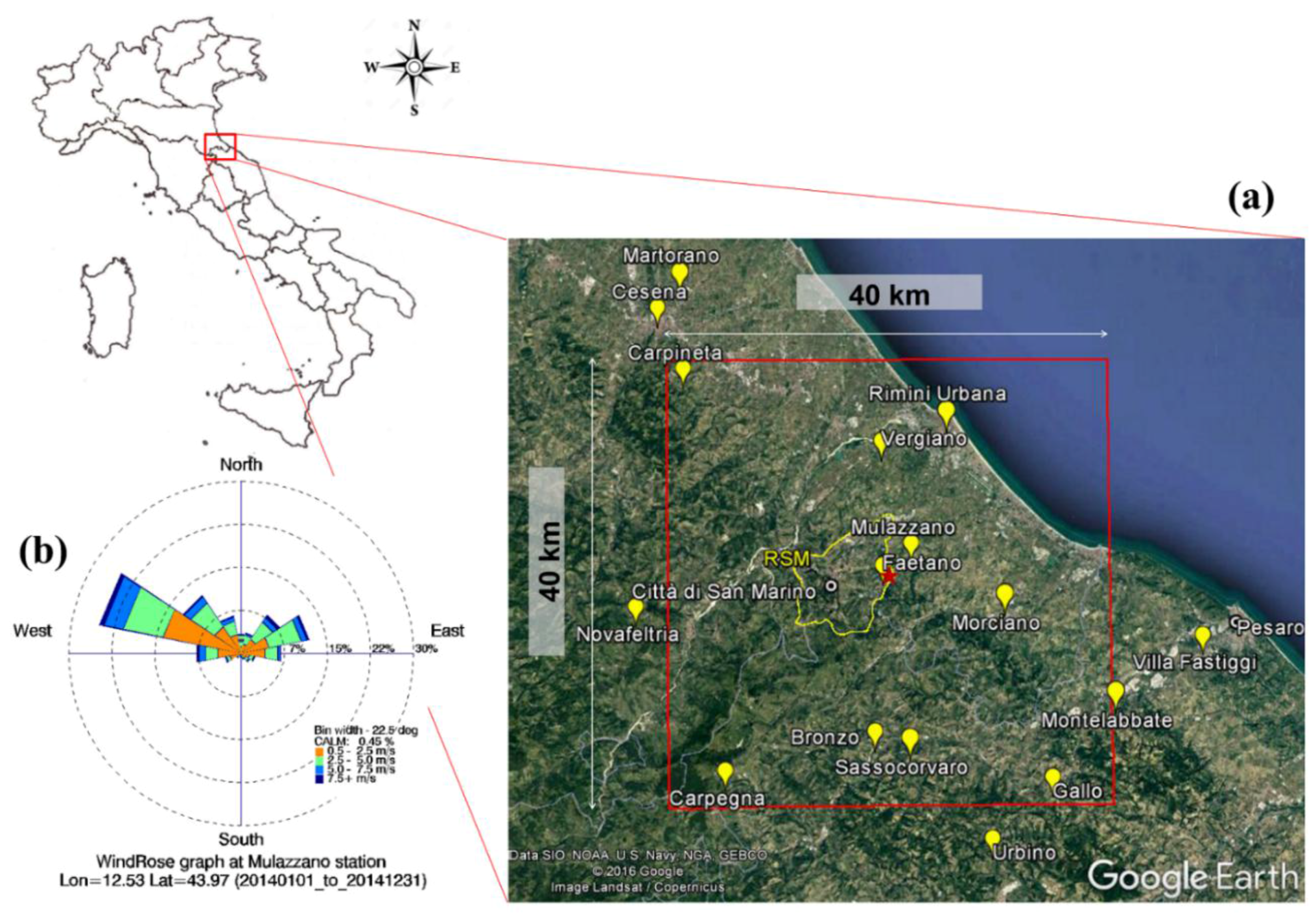
For the present study, a local scale simulation was performed: the diagnostic wind and temperature fields were computed over the spatial domain of 40 × 40 km² (Figure 1a), divided into a horizontal grid of 200 m square cells, and into a vertical grid of 10 layers from the ground to 1500 m above ground level. The pollutants concentration fields were computed over two spatial domains, the former of 40 × 40 km² divided into a horizontal grid of 200 m square cells, and the latter of 20 × 20 km², with a spatial resolution of 100 m. For both, the studied domain is centered at the release source point, i.e., the location of power plant stacks. Each single stack is simulated as an independent emitting source; the stacks have the same location at the simulation spatial scale. For the computation of the pollutant concentration vertical profiles, a vertical grid of 10 layers from the ground to 1500 m was used. The thickness of the first layer is set to 10 m, starting from the ground level. The emission sources of the power plant were simulated as a non-stop continuous release source points.

Lagrangian models are the used to properly simulate the pollutant dispersion in a complex terrain [14,15,17,19,20,21]: SPRAY does not include atmospheric photochemical processes, and only few models coupling Lagrangian dispersion with atmospheric chemistry exist in the literature of [32,33,34]. This study aimed to assess the impact of NO_x stack emissions on local air quality: since regulatory emission limits for combustion plants are set for NO_x (2010/75/UE), while for air quality are set for NO₂ (2008/50/EC), the simulation of NO_x dispersion represents a conservative and precautionary approach, since NO_x includes both NO₂ and NO. Moreover, the impact of emissions is highest in winter, when photochemistry is at its minimum, consistently with the conservativeness of the approach used, but with a lower simulation bias by neglecting the NO_x reactivity.

The year 2014 was chosen as reference period, being the most recent year not affected by the El Niño phenomenon. Both experimental and simulated meteorological data were used as input data for the meteorological model. The measured meteorological data were obtained by 16 ground-based meteorological stations of the Italian Environmental Agency network surrounding the power plant site in RSM, as mapped in Figure 1a. The wind rose graph for the meteorological ground station of Mulazzano (the closest to the source), for the year 2014 of hourly-measured wind data is reported in Figure 1b. The wind rose shows that the wind climate in the site is driven by mesoscale circulation, mainly characterized by moderate winds blowing from North West-West and, with lower frequency, from North East-East.

The simulated input data consist of a vertical wind profile close to the source point provided by the mesoscale COSMO atmospheric model (LAMA dataset), operating by Arpae Emilia Romagna [35,36]. The simulation domain for Italian application of COSMO covers an area of about 2000 × 2000 km² with a horizontal resolution of 7 km. The LAMA dataset covers the central part of the COSMO domain, with an area of 1200 × 1200 km².

Ground elevation data were provided by the Shuttle Radar Topography Mission through United States Geological Service (USGS), sampled at 3 arc-seconds, with a resolution of about 90 m (Version 4.1), while the land use/land cover (LULC) dataset was extracted by the European CORINE Land Cover (CLC) 2012 inventory [37]. To fulfill the requirements of SPRAY, the 44 LULC classes provided in the third level classification of the CLC were grouped in 21 classes [38].

5. Simulation Periods and Meteorological Conditions

In order to include all typical meteorological situations for the investigation domain, the simulations were performed considering both a period favorable to air pollution buildup (worst-case scenario) and three 10-day periods representative of different atmospheric dispersion conditions for the year 2014. Overall, the study covers two cold season periods featured by meteorological conditions leading to minimal dispersion of pollutants, and two summer periods featured by the highest atmospheric temperatures and maximum dispersion for the test year. This conservative approach is mainly suited to investigate the potential role of stack emissions in the exceedance of air quality regulatory limits (see

Table 2. Air quality limits for NO₂ and CO (D. Lgs. 155 13/08/2010).

	Limit Values for the Protection of Human Health
NO2	average hourly concentration not to be exceeded more than 18 times a calendar year	200 µg m−3
NO2	average concentration per calendar year	40 µg m−3
NO2	alarm threshold: average hourly concentration for 3 consecutive hours	400 µg m−3
CO	maximum average daily concentration—average over 8 h	10 mg m−3

for limits for NO₂ and CO, D.Lgs. 155 13/08/2010, implementation of 2008/50/EC [13]).

5.1. The Most Critical Period for Air Quality in 2014

The air pollution network of Italian Environmental Agency showed that the period between 11th and 20th March 2014 was highly critical for air quality in the neighboring regions of Emilia Romagna and Marche in 2014 [39,40]. In this period, intense anthropogenic emissions combined with adverse meteorological conditions, favoring the air pollution buildup in the first layer of the atmosphere. In March 2014, daily mean PM₁₀ from the air quality network exhibited several exceedances of the daily regulatory limit (50 μg m⁻³), and recorded the annual peak in the nearby provinces of Rimini and Forlì-Cesena. By the examination of the origin of air masses with HYSPLIT back-trajectory model [41] during this period, the contribution by Saharan dust from Northern Africa was excluded [42]. Hence, the ten days from March 11th and March 20th 2014 were chosen as the period of investigation of a worst-case scenario.

The main meteorological variables potentially affecting atmospheric pollutant level are: Precipitable Water (PWAT), Wind Speed (WSPD), Temperature (TSFC), and the Planetary Boundary Layer Depth (ZPBL). These parameters were firstly obtained from 6-hourly analysis files from the NOAA National Center for Environmental Prediction (NCEP) Global Forecast System (GFS) [43]. For each day of the investigated period, four analysis files were available at 00, 06, 12, and 18 UTC, calculated at the source coordinate (43.97° N–12.53° E).

In Figure 2, the trends of ZPBL (a), TSFC (b), and PWAT (c), for the month of March 2014, are reported. This period showed low PBL depth values, including the monthly minimum, mainly during the nighttime, when the PBL decreases due to the lack of rising thermals from the surface. An almost total absence of a cloud cover over the domain, and a total absence of rainfall events, with extremely low precipitable water values (c) was observed during the period. As further relevant consequence of low values of precipitable water, an increment of the air pollution daily mean concentration in the area was recorded.

Figure 3a shows the hourly wind rose at the source location for the critical period, obtained from the wind field computed by the diagnostic model SWIFT. The wind rose in Figure 3b, shows a sea breeze system featured by winds blowing from W-SW at night, gradually shifting to an E-NE origin at daytime, and wind calm (wind speed < 0.5 m s⁻¹) after sunset at 18 UTC. Wind speeds results were low (0.5–2.5 m s⁻¹), except for the first and last day of the period, when they occasionally reached 5 m s⁻¹. Frequent wind calms occurred during this period, both after sunset and at night (30%).

According to the wind roses in Figure 3b, the most notable breeze features are the relatively rapid increase in wind speed from about 1.5 m s⁻¹ during the night and early morning hours to about 3 m s⁻¹ at 12 UTC. This abrupt wind speed increase is accompanied by a wind shift from a land breeze during the night and a sea breeze during the diurnal hours.

In addition to the meteorological parameters trends analysis, the atmospheric temperature profile by radio-sounding at San Pietro Capofiume was investigated, being the nearest available profile. The data, (not shown) provided by the University of Wyoming, highlighted a thermal inversion at about 1000 m of altitude at nighttime, during the critical period. This condition of atmospheric stability determined near-surface stagnation and buildup of pollutants.

5.2. Summer and Fall Representative Periods during the Year 2014

The analysis of the atmospheric dispersion included also periods in summer and fall 2014, in order to have a clear picture of the atmospheric dispersion in frequent meteorological conditions. Considering the annual air quality reports for the simulation domain [32,33], it was possible to characterize the summer and the fall periods to be investigated.

Two periods in June 2014 were considered as representative of the summer season. This month is characterized by high values of ZPBL (between 600 and 1900 m at 12 UTC), more than one consecutive day of sunny days with high temperature at daytime at the surface and few rain episodes. June 6th to June 15th, 2014, and June 19th to June 28th were selected as periods: low PBL depth and high PBL depth occurred in the former and in the latter, respectively. In the second half of June, intense wind speed occurred much more frequently than in the other periods (Figure 4a,b). This meteorological condition, combined with high values of PBL depth, may lead to a good atmospheric dispersion of the emitted pollutants. The summer was featured by a land-sea breeze system similarly to March.

November 2014 was set as a representative period for fall. This period was characterized by low ZPBL from November 8th to November 17th both at daytime (about 500 m at 12 UTC), and during the nighttime. Nevertheless, this phenomenon was not observed in the last three days, where the PBL depth reaches about 1000 m at 12 UTC. In this period the wind at the source point blew mainly from East-Northeast and also from West-Northwest, with speed mainly lower than 5 m s⁻¹ (Figure 4c). Calm conditions corresponded to about 8% of the observations. Intense wind speed (7.5 m s⁻¹) events were recorded from Northwest-West. The effect of local sea breeze circulation was not negligible, but it was less evident than in the spring and the summer periods described above.

6. Results and Discussion

For each period of analysis, the simulations were performed with an hourly time-step, according to the hourly meteorological input data. The plant was considered under steady-state operation, where its specific features are reported in Table 1.

As introduced in Section 2, the emitted NO_x concentration in dry exhaust gas (based on 15 % O₂) was set to 50 mg N m⁻³, as provided by the manufacturer, and slightly below the emission limit of 52 mg Nm⁻³, and CO concentration in dry exhaust gas (based on 15% O₂) was assumed equal to the regulatory limits (100 mg N m⁻³).

The simulated concentrations were compared with the air quality limits for NO₂, and CO (D.Lgs. 155 13/08/2010) reported in Table 2. Since the simulated CO ground concentration results were always largely lower than the regulatory limits, they were omitted.

It is worth noting that the maps in Figure 5, Figure 6 and Figure 7 and all further analysis include only simulated ground concentrations higher than 1 μg m⁻³; these latter concentrations were referred in the rest of the text as plume concentrations. The power plant stacks, due to the map resolution, have the same location at the map scale (red star) and represent the center of the domain.

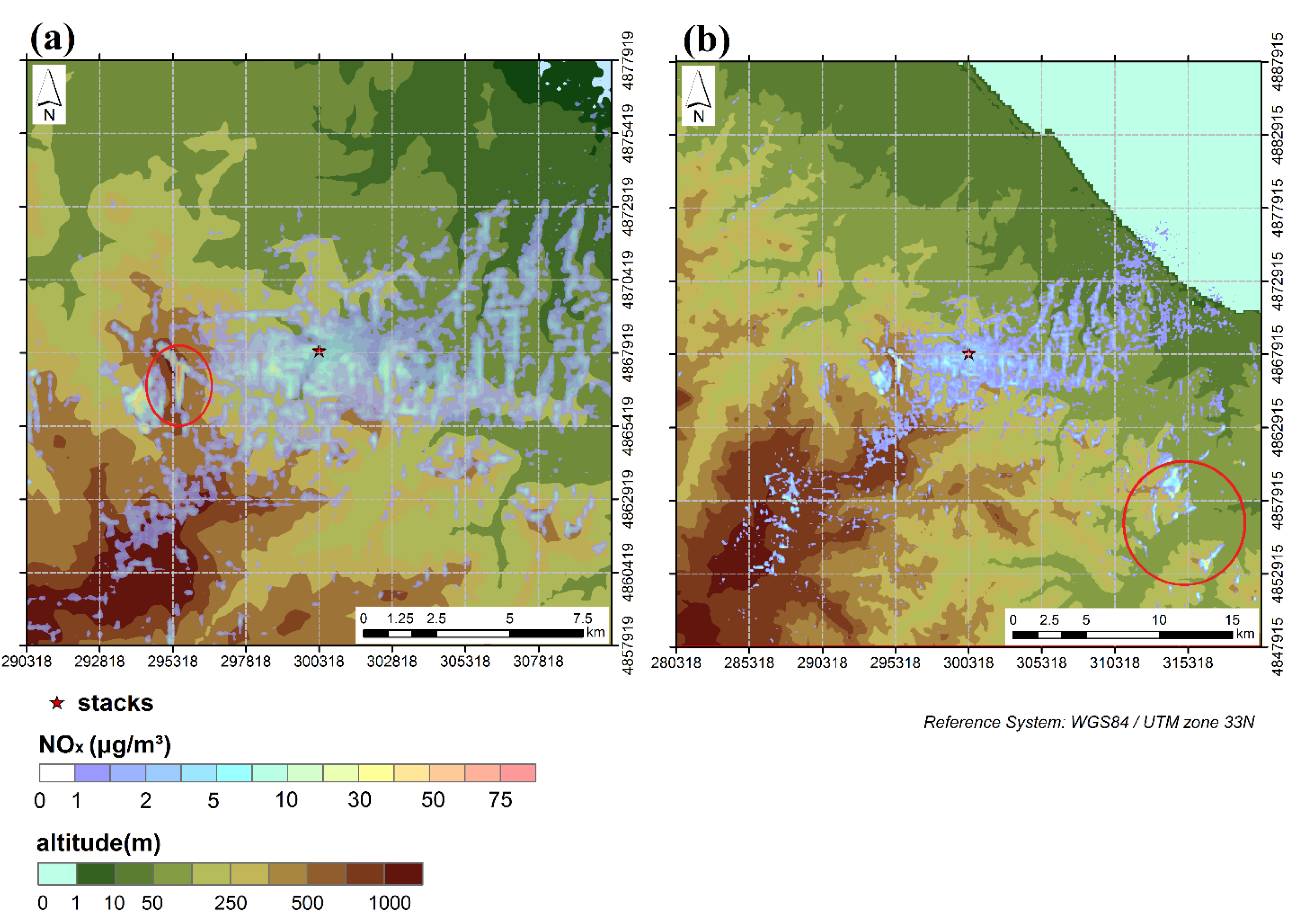
6.1. NO_x Average Hourly Concentration Maps for the Most Critical Period

The simulation was performed at first for the most critical period, ranging from March 11th to March 20th, 2014. Figure 5 shows the maps of the plume emitted by the power plant, as average hourly NO_x concentration in the first atmospheric layer (10 m) mapped over the Digital Terrain Model (DTM) of the spatial domain (20 × 20 km² in Figure 5a and 40 × 40 km² in Figure 5b respectively). The simulated plume in Figure 5a appears stretched approximately from West to East over the 20 × 20 km² domain. The simulated NO_x concentrations were compared to air quality limits for NO₂ (Table 2). The average hourly NO_x concentration in the investigated period ranges from 1 μg m⁻³ to a maximum value of 65 μg m⁻³, at about 5 km West from the power plant and close to the Mount Titano relief. Mount Titano represents a physical barrier to the plume dispersion, causing air stagnation with local accumulation of the power plant emissions. The maximum hourly average concentration (65 μg m⁻³) occurs over the Eastern slope of Mount Titano and next to San Marino City as highlighted in red in Figure 5a. The plume average concentration at ground over the domain is lower than 2 μg m⁻³, largely below the two regulatory limits for hourly peak (200 μg m⁻³) and annual mean (40 μg m⁻³) NO₂ concentration. The vertical profiles of NO_x average hourly concentration along the western plume stretch for the critical period were investigated (not shown). The concentration vertical profiles calculated at 1, 3, 5, and 10 km from the release source show the maximum concentration at about 700 m of altitude, at 5 km from the source, where the plume impacts the steep slope of the Mount Titano. To better investigate the atmospheric dispersion towards the Adriatic Sea, the concentration field was also computed on a larger domain (40 × 40 km²), with a horizontal grid step of 200 m. Figure 5b shows the maps of average hourly NO_x ground concentration. The plume concentration for this larger domain were generally lower than the NO₂ regulatory limit, ranging from 1 μg m⁻³ to maximum values of about 90 g m⁻³, with an average plume value lower than 2 g m⁻³. 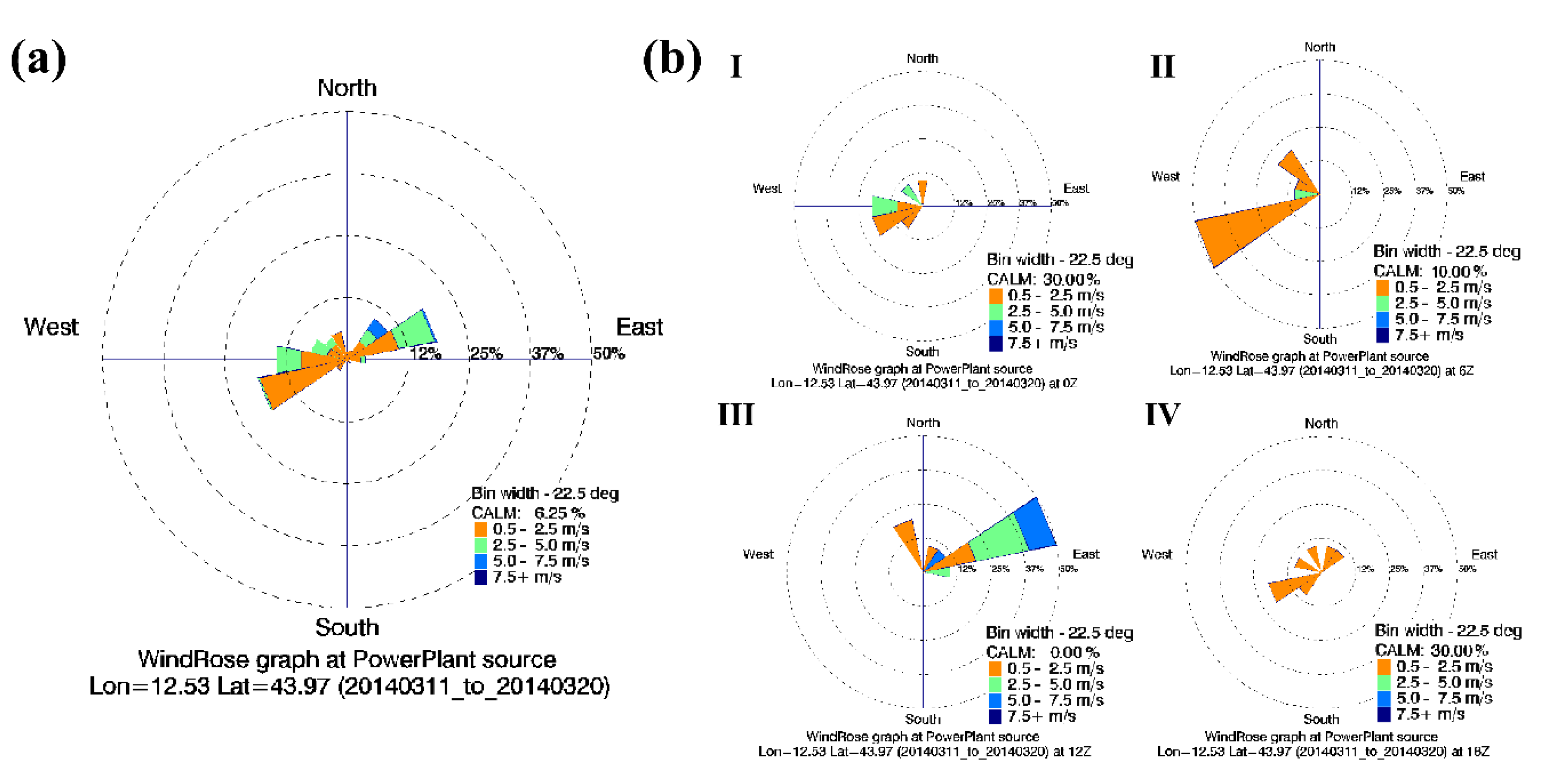In addition to the already mentioned concentration peak (65 g m⁻³) close to the Mount Titano, six non-contiguous cells ~25 km SE of the plant had a concentration peak of average hourly concentration between 40 g m⁻³ and 90 g m⁻³ (see the red circle in Figure 5b). At that greater distance from the stacks, the plume is dispersed upwards in the atmosphere and downwards to the ground, and natural obstacles (e.g., hills) may cause occasional concentration peaks. The concentration peak on the slope of Mount Titano is due to the recurrent Northeast-East winds, as shown by the wind rose in Figure 4a, while NW winds are responsible for the single scattered peaks occurring South-East of the plant (Figure 5b).

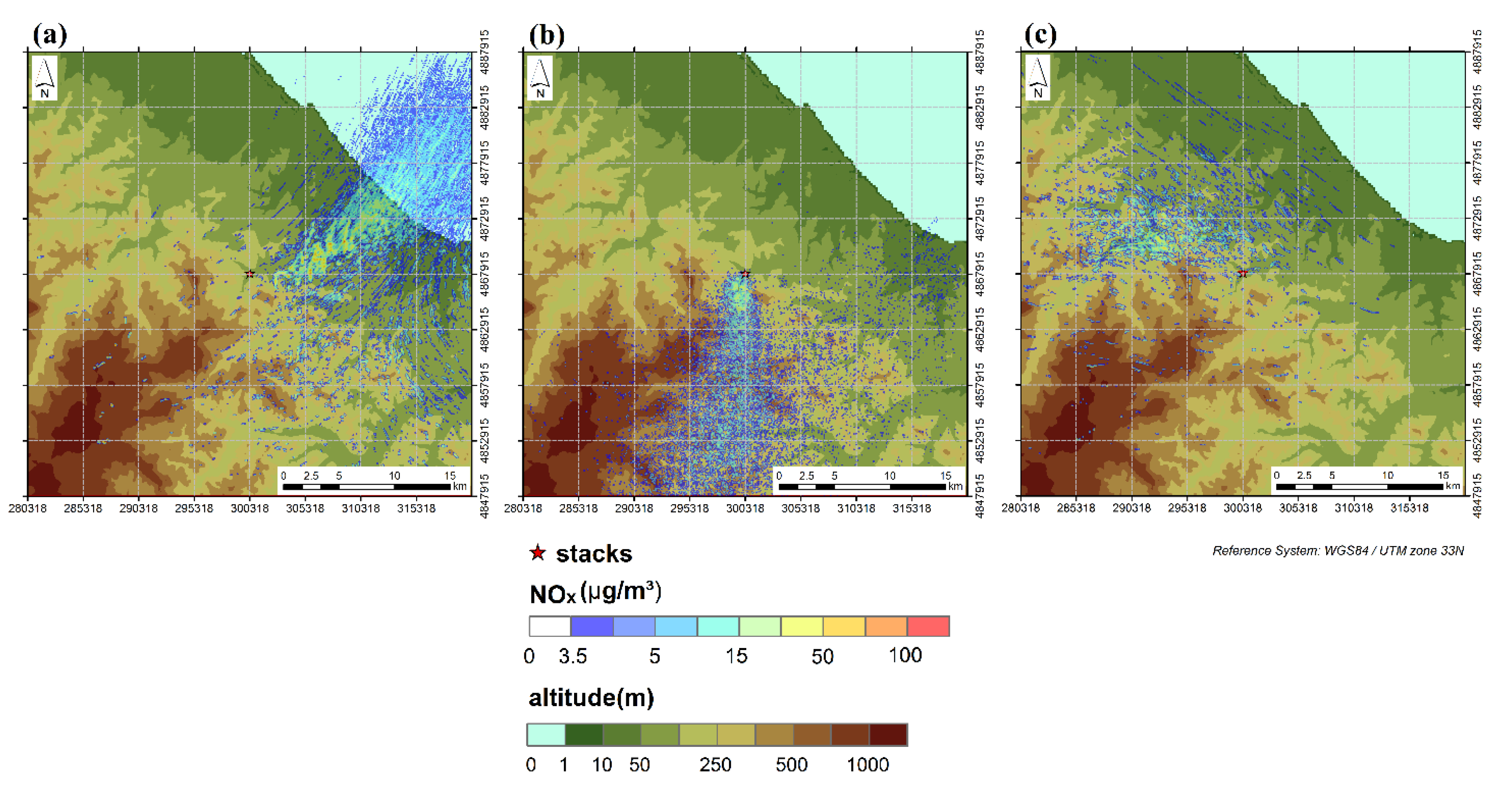
6.2. NO_x Concentration Maps at the Synoptic Hours

The wind roses previously reported (Figure 4b) show how the effects of local breeze circulation are important: at the four synoptic hours (00, 06, 12, 18 UTC), a predominant wind direction is evident (see Section 5.1). This effect was investigated on a particular day within the critical period: March 14th, 2014, as the most representative. The maximum average hourly NO_x ground concentration for March 14th, 2014, was 110 µg m⁻³, and occurred close to the Mount Titano, while the average plume value for the domain is equal to 2.2 µg m⁻³.

The maps of average hourly NO_x ground concentration at the four synoptic hours 00, 06, 12, 18 UTC on the spatial domain of 40 × 40 km² are reported in Figure 6a–c. A single map was provided for the two synoptic hours 00 and 06 UTC, due to their similar dominant winds from West-Southwest. At 00 and 06 UTC the plume moves East, while at 12 UTC the plume is transported South by the wind and finally, at 18 UTC, wind calm prevails. It is worth noting that this local sea breeze circulation effect should be considered in combination with the prevailing atmospheric circulation at mesoscale.

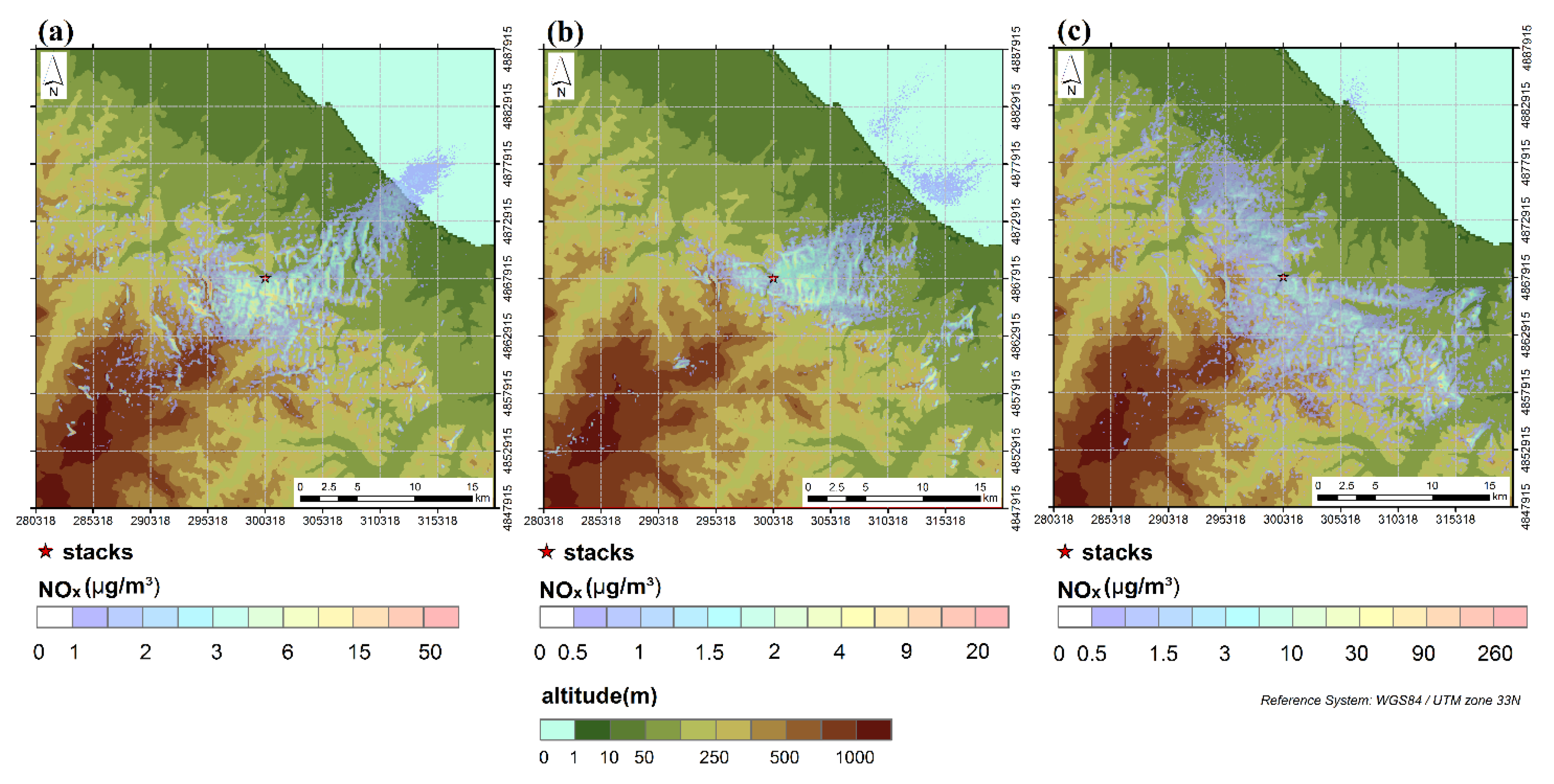
6.3. NO_x Average Hourly Concentration Maps for the Summer and Fall Periods

The average hourly NO_x concentration in the first atmospheric layer (10 m) in summer (from June 6th to June 15th, 2014 and from June 19th to June 28th, 2014) and in fall (from November 8th to November 17th 2014) periods was simulated considering both the smaller (20 × 20 km²) and the wider (40 × 40 km²) domain. The maps for the wider domain are here reported and discussed, as more representative.

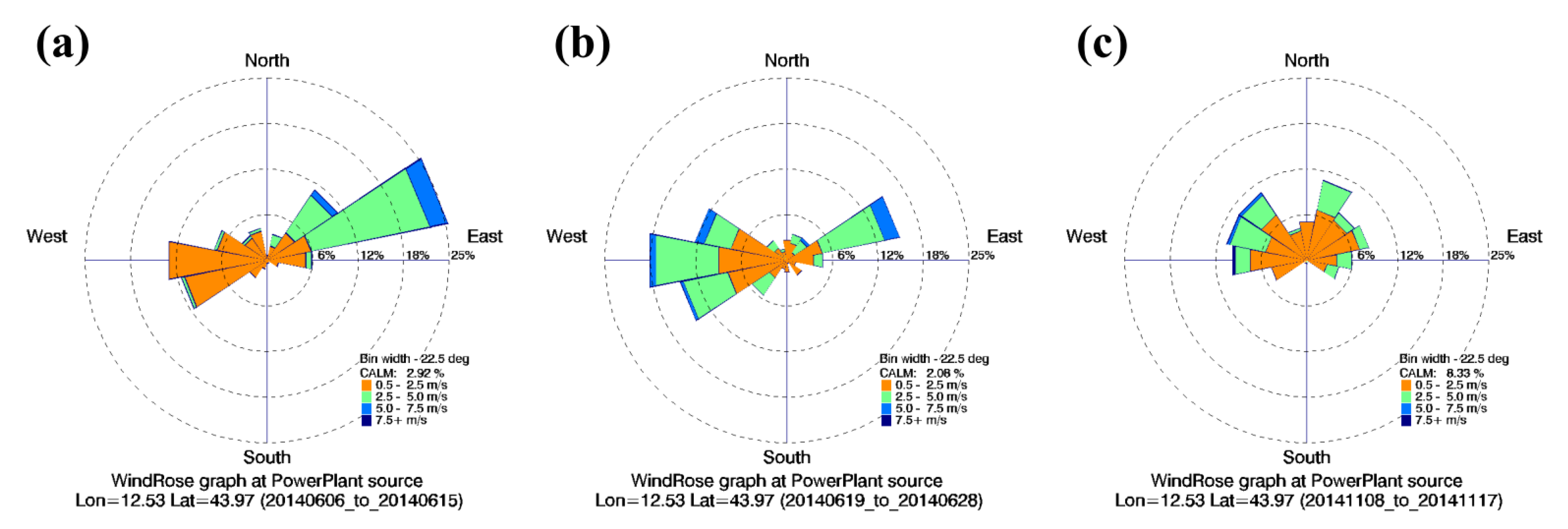
Figure 7a shows the maps of the plume emitted by the power plant mapped over the DTM on the wider domain for the first summer period. The plume appears stretched approximately from NE to SW, consistently with the wind rose in Figure 5a, where the much more intense winds blow from Northeast direction. Therefore, the plume is dispersed towards the Mount Titano on the West of the source. The average hourly NO_x concentration for the plume in this summer period ranges from 1 μg m⁻³ to a maximum of 77 μg m⁻³, obtained close to Mount Titano, slightly Southwest from it. The plume average value through the domain is about 2 μg m⁻³.

The plume for the second summer period (Figure 7b), is stretched approximately from West-Northwest to East, consistently with the wind rose in Figure 5b. Since in this period the Western winds are the most intense, the plume is mainly dispersed towards the Adriatic Sea coast. The average hourly NO_x concentration for the plume in this second summer period ranges from 1 μg m⁻³ to a maximum of almost 30 μg m⁻³, occurring at 15–18 km East South-East of the power plant; concentration values of about 12 μg m⁻³ are obtained on the Eastern slope of Mount Titano relief. The plume average value through the domain is lower than 2 μg m⁻³.

In Figure 7c the map of the plume for the fall period is shown: the plume is stretched approximately from Northwest to Southeast (see the corresponding wind rose in Figure 5c). In this period, the Northwest-West winds are the most intense, dispersing the plume towards the mountain relieves to the Southeast side of the source. The average hourly NO_x concentration ranges from 1 μg m⁻³ to a local maximum of almost 390 μg m⁻³, occurring 15 km Southeast of the power plant. Fifteen non-contiguous domain cells at 20–25 km SE of the plant showed high concentration with an average between 40 µg m⁻³ and 90 µg m⁻³; the area is impacted also during the critical period, when, however, the concentration peaks fall in different domain cells (Section 6.1). Concentrations of about 29 μg m⁻³ are on the Eastern slope of Mount Titano. The plume average value through the domain is about 2 μg m⁻³.

6.4. Pollution Roses and Exceeding of Regulatory Limits

The NO_x pollutant roses for the four simulation periods are shown in Figure 8a–d. The wind data for the source point at the plant stack elevation and the hourly NO_x ground concentration were used to obtain a conditional bivariate probability function (CBPF [44]): each CBPF estimates the probability that a specific concentration range is observed within a given wind sector (of 5 degrees width), depending upon wind speed. CBPFs in Figure 8 show the probability frequency of NO_x concentration higher than the hourly regulatory limit for each wind speed and direction class.

CBPFs were computed using wind data by the diagnostic model SWIFT at the source point, and the average simulated NO_x concentration in a 100 m × 700 m area over the Eastern slope of Mount Titano, where recurrent concentration peaks are expected. The concentration range used to compute CBPF considered levels larger than the regulatory limit of 200 μg m⁻³. Plots in Figure 8 show that in March (Figure 8a), the exceedances are triggered by moderate Eastern winds, in June (Figure 8b,c) exceedances have a very low probability, and in November, the exceedances over that small area of the Eastern slope of Mount Titano are related to wind calm and slow Northestern winds.

The outcome of CBPF was compared to the wind roses of each investigated period (Figure 3a and Figure 4a–c): CBPFs show the percentage of wind conditions that may be responsible of concentration peaks around the Mount Titano area, while the wind rose graph for the entire year 2014 (Figure 1b) shows that the frequency of the wind events blowing from Northeast-East in the year 2014 is of about 11%, while the calms correspond to less than 1% in the year. Therefore, the regulatory limit for average hourly NO₂ concentration is expected to be exceeded more than 18 times a calendar year, but limited to the focus area on the Eastern slope of Mount Titano. Considering only the simulation periods, in the focus area, the regulatory limit for NO₂ is exceeded 33 times in total (14 times in March, 13 in November, 2 and 4 in the two summer periods respectively). Nonetheless, in the nearby domain cells, NO_x concentration sharply decreases, with results largely lower than the regulatory limits. Consistently with CBPF (Figure 8), the 33 exceedances occur in presence of wind events blowing from Northeast-East and of wind calms.

7. Conclusions

The present work investigated the impact assessment of the NO_x atmospheric emissions from a cogeneration plant, which will be installed in the area of Republic of San Marino, considering the regulatory limits for the combustion plants set by the Italian law. The environmental impact was performed via numerical simulations of atmospheric dispersion of the exhaust gases emitted from the cogeneration plant stacks and the results further analyzed by statistical models. The study considered both a worst-case meteorological scenario (critical period) in March 2014, and two summer and one fall representative period in 2014. The power plant was assumed under continuous non-stop operation. The resulting maps of hourly average simulated concentration at the ground level (i.e., in the first atmospheric layer starting from the ground, 10 m thick) showed values largely lower than the regulatory limits for air quality for NO₂.

The results of the simulations for the largest of the two simulation domains (40 × 40 km²), both for the critical and the representative periods, showed at the ground level average hourly concentration fields featured by very low values, with local single peaks where the emission plume impacts the ground reliefs. These peaks occur in two different areas of the domain depending on the simulation period: an area over the SE slope of Mount Titano showing recurrently large concentration levels both in March and in the June periods, and an area at 20–25 km SE of the power plant. Peaks in this latter area occur in different domain cells depending on the simulation period, without the evidence of a recurring accumulation point, therefore, they should not give rise to persistent pollutant buildups.

Nevertheless, the NO_x plume average concentration over the largest investigated is ca. 2 μg m⁻³. The wind rose graph for the entire year 2014 showed that the frequency of NE winds causing a concentration peaks over the slope of Mount Titano was of about 11%, and that the frequency of NW winds causing high concentration SE from the power plant is of about 12%, while wind calm frequency is lower than 1% per year. The pollution roses show that the regulatory limit for average hourly NO₂ concentration is already exceeded more than 18 times during the investigated period, but limited to a steep area on the cliff of Mount Titano. Therefore, the power plant emissions are expected to meet the air quality limit for NO₂ hourly average concentration (200 μg m⁻³) throughout the investigated domain, except around the area close to Mount Titano, where the hourly limit for NO₂ is expected to be exceeded. Due to its location with respect to the source, this area may be considered the most exposed to a local accumulation of pollutants emitted from the power plant. Yet, it is fortunately not a residential area, due to its steep morphology. Similarly, the power plant emissions will be expected to meet the annual limit (40 μg m⁻³) for mean annual NO₂ throughout the investigated domain, except around the area close to Mount Titano. The limit for NO₂ annual mean is expected not to be exceeded in the area SE of the power plant, even if several concentration peaks occur there, because these single peaks (in scattered domain cells) mainly occur in different areas of the domain for each simulated period, without the evidence of recurring accumulation points.

This study highlighted how the innovative combined use of a Lagrangian dispersion model (SPRAY) and of statistical models leads to an accurate assessment of the environmental impact by power plant emissions over a complex terrain and under unsteady wind conditions. The project includes the use of cogeneration in combination with heat-pump technology and plug-in vehicles, as part of a renewable electric grid, in order to make San Marino a “smart” society [23], with a more robust energy infrastructure which might drive economic growth.