Article

Exploring the Coupling and Decoupling Relationships between Urbanization Quality and Water Resources Constraint Intensity: Spatiotemporal Analysis for Northwest China

1
Institute of Geographic Sciences and Natural Resource Research, Chinese Academy of Sciences, Beijing 100101, China
2
Key Laboratory of Regional Sustainable Development Modeling, Chinese Academy of Sciences, Beijing 100101, China
3
College of Resources and Environment, University of Chinese Academy of Sciences, Beijing 100049, China
*
Author to whom correspondence should be addressed.
Sustainability 2017, 9(11), 1960; https://doi.org/10.3390/su9111960
Submission received: 7 September 2017 / Revised: 20 October 2017 / Accepted: 24 October 2017 / Published: 27 October 2017
(This article belongs to the Section Sustainable Urban and Rural Development)

Abstract

:
China is faced with great challenges for its low urbanization quality and high water stress. Moreover, the relationship between urbanization quality and water resources is still ambiguous. Therefore, we firstly constructed an urbanization quality index (UQI) and a water resources constraint intensity index (WRCI) by a fuzzy comprehensive evaluation method with multi-objectives and multi-hierarchies. Secondly, based on the concept and method of “coupling” and “decoupling”, we provided a method to explore the coordinated and uncoordinated relationships between UQI and WRCI from a spatiotemporal perspective. Finally, we used the statistical data of 51 prefecture level regions in Northwest China from the period 2000–2014 to analyze the spatiotemporal variation of the coupling and decoupling relationships between UQI and WRCI. Results show that, the UQI and WRCI in the whole Northwest China both belonged to low level, and that they had achieved strong decoupling during 2000–2014. However, the coupling and decoupling relationships between UQI and WRCI in Northwest China had great spatial disparity. From the HL-type regions (regions with high UQI & low WRCI) and strong decoupling type regions, we can find key development areas of Northwest China, where the relationships between UQI and WRCI were optimal and coordinated. From the LH-type regions (regions with low UQI & high WRCI) and strong negative decoupling type regions, we can find key problem areas, where the relationships between UQI and WRCI were the worst and uncoordinated. Our study developed an effective method for evaluating the sustainable development level of urbanization constrained by water resources in Northwest China and similar regions, which is significant for the New-Type Urbanization research in China.

1. Introduction

Rapid urbanization is usually accompanied by explosive increase of urban population, widespread economic growth, linear decreasing of ecosystem services and serious water scarcity, especially in arid and semi-arid regions [1,2,3,4,5]. This is evidenced by river and lake drying, land degradation, biodiversity loss, ecological migration, living standard declining, etc. [5,6,7,8]. These changes have made scarce water resources as an even more significant restriction on regional urbanization, socio-economic development and environmental conservation [9,10]. There are complicated interactions between urbanization and water resources [11,12]. On the one hand, urbanization has both positive and negative effects on water resources utilization. It may bring more urban water resources demand, hydrological deterioration and environment degradation [13,14], as well as improvement of water use efficiency [15]. On the other hand, water resources can sustain and constrain the urbanization process at the same time [11,12]. Many scholars have realized the importance of the coordinated development between urbanization and water resources utilization [15]. However, much concern is still about the relationship between urbanization quantity and water resources amount, e.g., population urbanization ratio and total water consumption [15,16,17]. The relationship between urbanization quality and water resources is less considered. Therefore, we tried to construct an urbanization quality index (UQI) and a water resources constraint intensity (WRCI) to explore their coupling and decoupling relationships.
Urbanization quality describes the superiority and inferiority of the urbanization process and is often the “contradictory” pair of urbanization quantity [18]. In China, urbanization quality was formerly defined as urban modernization and urban–rural integration [19]. However, due to the difference of study perspectives and objectives, the definitions and the comprehensive measurement indicator system were much different [20,21,22,23,24,25]. During the 18th National Congress of the Communist Party of China in November 2012, the Chinese government put forward the concept of New-Type Urbanization, highlighting the necessity to transform urbanization mode from “quantitative growth” to “quality improvement”. In March 2014, China’s National Development and Reform Commission released the “National New-Type Urbanization Plan (2014–2020)”. It aims at promoting people-oriented urbanization and improving urbanization quality [18]. However, how to define and measure the urbanization quality has not been authoritatively released by the Chinese government. It has become a key issue for New-Type Urbanization research [18].
Water resources constraint intensity refers to the conflict degree between water scarcity and human activities [26]. Some scholars have provided a huge amount of single or comprehensive indicators and indexes to assess the relationship between water scarcity and human activities [27,28,29]. For example, Water Stress Index (WSI) which is defined as average per capita water availability per year, and Water Exploitation Index (WEI) which is defined as the percentage of freshwater withdrawal with respect to the long-term mean annual freshwater resources, have been widely used [30,31,32]. Water Poverty Index (WPI) [33,34], Integrated Water Stress Index [35,36], Water Scarcity or Shortage Index [37,38], Water Resources Carrying Capacity Index [39,40], Water Security Index [41,42] and Human-Water Harmony Index [27] are all the most commonly comprehensive indicators. However, each of them has been defined under different assumptions or conditions. Therefore, its applicability may be limited, and there is not a unique indicator suitable for all areas of study [29]. The best choice depends on the indicators which are under consideration and the preferences of the decision maker [28]. Moreover, when applied to the specific Chinese situations, the above composite indexes need to incorporate both social and culture characteristics [27].
As urbanization is closely related to economic growth and water is an important natural resource as well as a key element of eco-environment, previous studies on the coupling and decoupling relationship between urbanization (or economic growth) and eco-environment (or natural resources) may provide useful references. For example, the coupling mechanism and rules between urbanization and eco-environment have been analyzed [43,44]. The coupling coordination model between urbanization and eco-environment have been constructed and applied in various regions [45,46,47,48,49]. The concept of “decoupling” [50] have been used to analyze the relationships between water uses and economic development [51], economic growth and environmental degradation [52,53], economic development and carbon emissions [54,55,56], carbon emissions and transportation [57], etc. However, most previous studies focused on the quantity of the coupling and decoupling relationships between two variables for one region, i.e., how much one variable may connect or disconnect with the other in a certain area. Few studies focused on the spatiotemporal type of the coupling and decoupling relationships.
Therefore, to contribute in filling the above literature gaps, we firstly constructed an urbanization quality index (UQI) and a water resources constraint intensity index (WRCI) by a fuzzy comprehensive evaluation method with multi-objectives and multi-hierarchies. Secondly, we drew lessons from the concept and method of “coupling” and “decoupling”, and provided a method to explore the coordinated and uncoordinated relationships between UQI and WRCI from a spatiotemporal perspective. Finally, we used the statistical data of 51 prefecture level regions in Northwest China during 2000–2014 to analyze the spatiotemporal variation of the coupling coordinated relationships between UQI and WRCI, so as to find the key problem regions and put forward some policy implications.

2. Materials and Methods
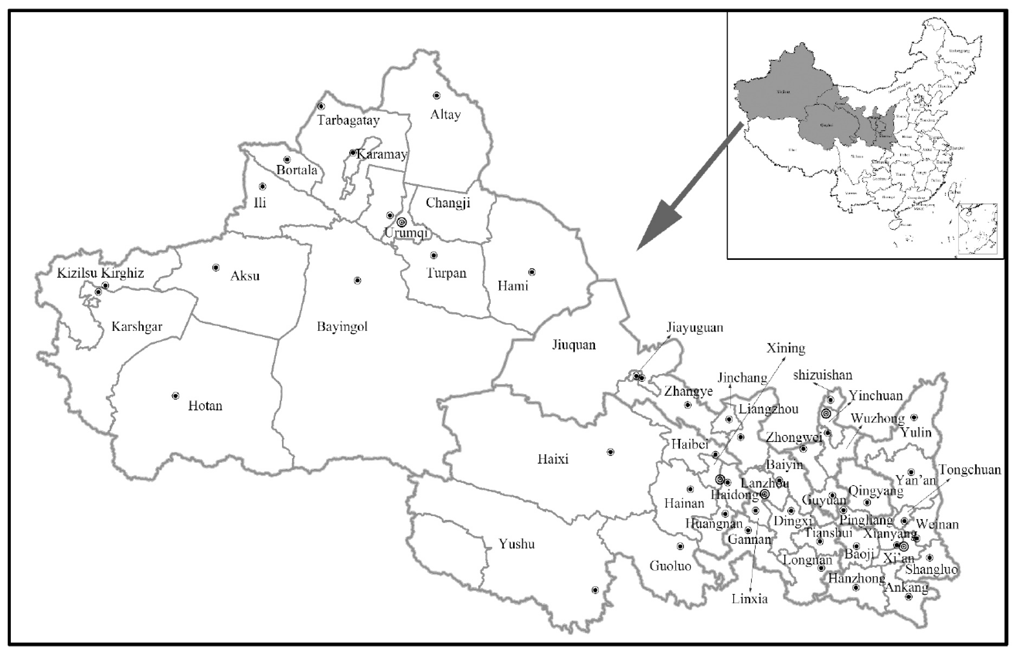
2.1. Study Area

Northwest China, located in in the hinterland of Eurasian continent, has a typical arid and semi-arid continental climate, which is characterized by little precipitation, high evaporation and a wide range of temperature [58]. It traditionally includes the provinces of Shaanxi, Gansu, Qinghai and the autonomous regions of Xinjiang and Ningxia, and has 51 prefecture level cities and autonomous prefectures (Figure 1). In 2014, it has an area of 3.1 million km2, occupying 32.44% of total area in China. However, its gross amount of water resources is 216.87 billion m3, only 7.95% of the national total. It has a population of 98 million, which accounts for 7.17% of China’s total. The Gross Domestic Product (GDP) is 3890 billion yuan, which accounts for 6.11% of China’s total. The population urbanization ratio, which is a frequently-used indicator for urbanization quantity, is 48.12%, and that in Ningxia, Shaanxi, Qinghai, Xinjiang and Gansu is 53.61%, 52.58%, 49.76%, 46.07% and 41.68% respectively. It indicates that Northwest China is in the accelerating development stage of urbanization. The annual average growth rate of GDP is 12.60% during 2000–2014, much higher than the national average of 9.87%. With rapid urbanization and economic growth, Northwest China has been suffering from severe water scarcity [59]. The gap between water supply and demand may continue to intensify in the future [60]. In the context of “the Belt and Road Initiatives” and New-Type Urbanization, it is of practical significance to improve urbanization quality and lessen water resources constraint intensity in Northwest China.

2.2. Indicator System of UQI & WRCI and Data Sources

To explore the coupling and decoupling relationships between urbanization quality and water resources constraint intensity, we firstly constructed an integrated indicator system to measure UQI and WRCI. The indicators were primarily selected according to the following general selection criterion [26,49]: (1) cover the components of urbanization quality and water resources constraint intensity based on their connotations; (2) choose the most cited indicators; (3) choose the simplest indicators to facilitate data collection, understanding and dissemination; and (4) choose the comparable indicators to reflect the dynamic changes in different areas. Subsequently, we used Pearson correlation analysis by a statistical analysis software named SPSS (Statistical Package for the Social Sciences) to filtrate the general indicator system, so as to eliminate the pertinence among different indicators. The comprehensive indicator system to evaluate UQI and WRCI is listed in Table 1.
Among the above indicators, most of them are frequently used and easy to understand except for 4 indicators. Specifically, the excellent rate of urban air quality is the proportion of days that urban air quality has reached the national grade II standard to the number of days throughout the year. The urban-rural income gap is the ratio of urban per capita disposable income to rural per capita net income. The urban-rural labor productivity gap is the ratio of the secondary and tertiary industry value-added created by per unit of the secondary and tertiary industry employment to the primary industry value-added created by per unit of the primary industry employment. The regional disparity of economic development is expressed by the Gini coefficient of per capita GDP in the region. For prefecture-level administrative units, per capita GDP of county-level administrative units is used. For the whole Northwest China, per capita GDP of prefecture-level administrative units is used. The calculation formula is as follows [61]:
G = 1 2 μ N 2 i = 1 N j = 1 N | y i y j |
where G is the Gini coefficient; | y i y j | is the absolute value of the difference of per capita GDP between any two study units; N is the number of study units; μ is the average value of per capita GDP in all study units.
The basic data in this paper include socio-economic data and water resources data for the 51 prefecture level regions in Northwest China during 2000–2014. The socio-economic data are all obtained in the past years China Statistical Yearbook for Regional Economy, China City Statistical Yearbook, China Statistical Yearbook (County-Level), statistical yearbook of Shaanxi, Gansu, Qinghai, Ningxia, and Xinjiang respectively. The water resources data are all obtained in the past years Water Resources Communique of Shaanxi, Gansu, Qinghai, Ningxia, and Xinjiang respectively. To make economic data comparable in time series, all the economic data are calculated at comparable prices in 2000. For the whole region of Northwest China, we summed up the original total quantity indicators of the 51 prefecture level regions firstly, and then calculated the average quantity indicators, except that the excellent rate of urban air quality was the average value of the 51 prefecture level regions.

2.3. Fuzzy Comprehensive Evaluation Method with Multi-Objectives and Multi-Hierarchies

2.3.1. Evaluation Criterion and Multi-Objective Threshold Values

In order to make the evaluation results comparable in spatial and temporal series, we define UQI and WRCI and their primary indicators between 0 and 1, and divide all of them equally into 5 types or levels: low, lower, medium, higher and high (Table 2). Based on this definition, we ascertain the corresponding six upper and lower threshold values for the secondary indicators through related literature review and experience of developed countries and regions (Table 2). For example, if per capita water resources in a certain research unit are between 500 and 1000 m3, the integrated index of natural endowment of water resources will be between 0.2 and 0.4, and its corresponding WRCI will be between 0.6 and 0.8, which means that the water resources constraint intensity is “higher”. Of course, the final integrated index of WRCI may be enhanced or reduced by other secondary indicators. For example, if water resources converted into the depth of surface runoff is not between 40 and 70 mm, the final type of the research unit may not be the “higher” level. It needs a comprehensive evaluation model under these circumstances.

2.3.2. Normalization and Multi-Hierarchies Aggregation Method

To make the secondary indicators have comparability in space and over time, we constructed a multi-objective fuzzy membership function based on fuzzy membership function [62] for normalization. It may translate them into a value score between 0 and 1 which represents the degree to which a decision objective is matched.
Specifically, suppose W = { w 1 , w 2 , , w a } and H = { h 1 , h 2 , , h b } . W is an indicator set, and H is a comment set. According to Table 2, there are 25 secondary indicators and 5 grading levels, so a = 25, and b = 5. h 1 represents low level and h 1 [ k 1 , k 2 ) . h 2 represents lower level and h 2 [ k 2 , k 3 ) . h 3 represents medium level and h 3 [ k 3 , k 4 ) . h 4 represents higher level and h 4 [ k 4 , k 5 ) . h 5 represents high level and h 5 [ k 5 , k 6 ] . Obviously, k 1 = 0, k 2 = 0.2, k 3 = 0.4, k 4 = 0.6, k 5 = 0.8, k 6 = 1. For any indicator i , its actual threshold values u 1 , u 2 , u 3 , u 4 , u 5 , u 6 correspond to the normalized threshold values k 1 , k 2 , k 3 , k 4 , k 5 , k 6 respectively. For example, If the actual value of an indicator is between u 1 and u 2 , the normalized value will be between k 1 and k 2 .
For positive indicators, the calculation formula is:
s λ i j = { k 1 x λ i j < u 1 k n + 1 k n u n + 1 u n × ( x λ i j u n ) + k n u n x λ i j u n + 1 ( 1 n 5 ) k 6 x λ i j > u 6
For negative indicators, the calculation formula is:
s λ i j = { k 1 x λ i j > u 1 k n + 1 k n u n u n + 1 × ( u n x λ i j ) + k n u n + 1 x λ i j u n ( 1 n 5 ) k 6 x λ i j < u 6
where s λ i j and x λ i j are the normalized value and actual value of indicator i in spatial unit j and in the year λ respectively.
Due to different importance of different indicators, we need to calculate the weights of the primary and secondary indicators before indicator aggregation. Analytic Hierarchy Process (AHP) is widely used to determine the relative weights of available alternatives, and the calculation steps are as follows [67,68,69,70,71]:
Firstly, we should structure the complex issues in a hierarchical order and construct the pairwise comparisons judgment matrix A = { a i j } n × n according to the relative significance of attributes on fundamental scale from 1 to 9.
A = ( a 11 a 12 a 1 n a 21 a 22 a 2 n a n 1 a n 2 a n n )
where n denotes the number of attributes, i [ 1 , n ] , j [ 1 , n ] , a i j = 1 / a j i .
Secondly, Matrix B = { b i j } n × n is obtained by normalizing every column of A . The normalization procedure is as follows:
b i j = a i j / i = 1 n a i j
Thirdly, b i is obtained by calculating the sum of every column of matrix B .
b i = j = 1 n b i j
Fourthly, the weight of indicator i is p i :
p i = b i / i = 1 n b i
P = ( p 1 , p 2 , , p n ) T is the approximate characteristic vector of A . Consistency check should be carried out to check the reliability of the result.
A P = A × P = ( A P 1 , A P 2 , , A P n ) T
Calculate the approximate maximum Eigen value λ max :
λ max = 1 n i = 1 n ( A P ) i p i
Calculate the Consistency Index (CI):
C I = λ max 1 n 1
Calculate the Consistency Ratio (CR):
C R = C I R I
where RI is the random index. The values of RI are listed in Table 3.
Generally, the consistency of judgment matrix is acceptable when C R 0.1 . Otherwise, the judgment matrix must be rectified until the Consistency Ratio reaches the acceptable range.
Though AHP provides a comprehensive and rational framework to deal with complex decisions, it may cause useful information of some indicators to be lost [26,72]. Therefore, it is necessary to use entropy technology to amend the weight of each indicator calculated by AHP. Here is the detailed procedure [26,72]:
Firstly, information entropy of the indicator i is e i :
e i = 1 ln ( n ) j = 1 n ( b i j ln b i j )
where b i j is calculated by Equation (5).
Secondly, the entropy redundancy of the indicator i is g i :
g i = 1 e i
Thirdly, the information weight of the indicator i is v i :
v i = g i / i = 1 n g i
Finally, the indicator weight amended by entropy technology is r i :
r i = v i p i / ( i = 1 n v i p i )
where p i is the weight of indicator i calculated by AHP using Equation (7).
Subsequently, we can use weighted aggregation to calculate the integrated indexes of the primary indicators and UQI and WRCI. To be simplified and concise, we only listed the formula to compute the UQI or WRCI.
F λ j = k = 1 m i = 1 n ( p k l × p i k × s λ i j )
where F λ j is UQI or WRCI in spatial unit j and in year λ ; p i k is the weight amended by entropy technology of indicator i to its primary indicator; p k l is the weight amended by entropy technology of the primary indicator to UQI or WRCI; m and n are the number of indicators in the corresponding hierarchy respectively.

2.4. Coupling and Decoupling Method from a Spatiotemporal Perspective

2.4.1. Spatial Coupling Classification Method

The concept of “coupling” originated in the field of physics, which defines a phenomenon in which two or more indicators impact on each other through various interactions [43,44,45,46,47]. UQI and WRCI are both comprehensive and complex indexes. They may impact on each other through their primary and secondary indicators indirectly. However, they do not impact on each other directly. In other words, they may have no direct causal relationship theoretically. Therefore, the quantitative relationship between these two variables may lose its real meaning. However, we may use spatial coupling type to reflect the coordinated relationship between UQI and WRCI. That’s to say, for a certain region, when the UQI is high and the WRCI is low, it is a key development area with HL-type. When the UQI is low and the WRCI is high, it is a key problem area with LH-type. When the UQI and WRCI are both high (or both low), it is a common problem area with HH-type or LL-type.
According to the grading criterions of UQI and WRCI in Table 2, there are five categories of UQI and WRCI respectively. Thus, there could be 25 kinds of coupling relationship between UQI and WRCI. To simplify the classification, taking 0.5 as the dividing line, we divided UQI and WRCI into high level (H type) and low level (L type) respectively. Subsequently, there are four spatial coupling types in total (Table 4).

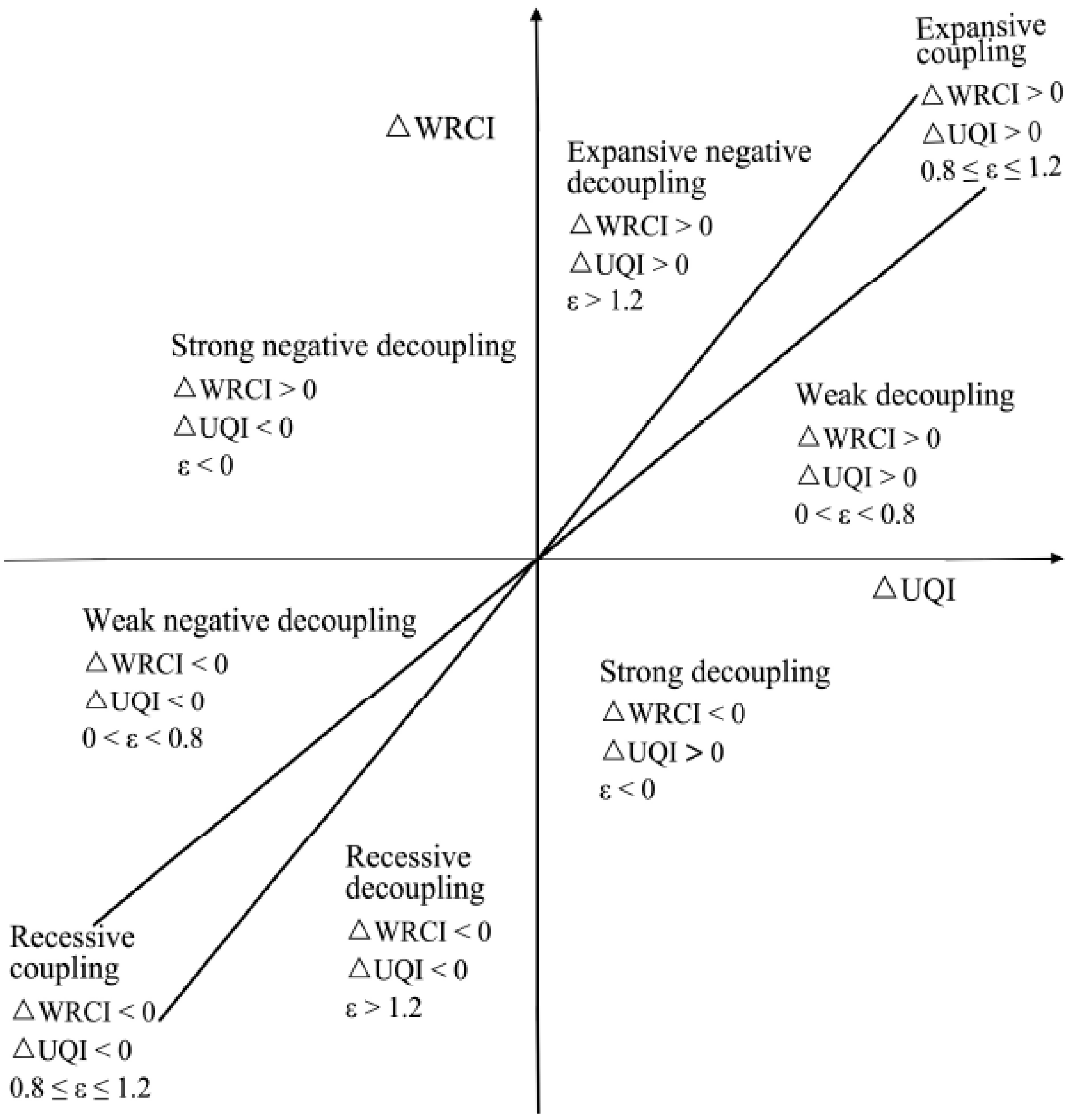
2.4.2. Temporal Decoupling Classification Method

The concept of “decoupling” also originated from physics, which means dissociating the relationships among some physical variables [50,51,52,53,54,55,56,57,73]. Tapio (2005) [54] defined decoupling index based on the concept of elasticity analysis and provided eight logical possibilities for decoupling states, namely weak decoupling, expansive coupling, expansive negative decoupling, strong negative decoupling, weak negative decoupling, recessive coupling, recessive decoupling and strong decoupling.
Theoretically, the changes of UQI and WRCI may have no direct causal relationship, and the quantitative relationship between these two variables may lose its real meaning. However, we may use the decoupling index to reflect the temporal decoupling type between the changes of UQI and WRCI for a certain region. The specific calculation forum is as follows:
ε = Δ W R C I Δ U Q I = ( W R C I t W R C I 0 ) / W R C I 0 ( U Q I t U Q I 0 ) / U Q I 0
where ε denotes the decoupling elastic coefficient; Δ W R C I and Δ U Q I denote the changes of water resources constraint intensity and urbanization quality index between a base year 0 to a target year t respectively. The decoupling state judgment is shown in Figure 2.
Weak decoupling state means the situation when the growth of WRCI is lower than the growth of UQI. Expansive coupling state means the situation when the growth of WRCI is approximately equal to the growth of UQI. Expansive negative decoupling state means the situation when the growth of WRCI is higher than the growth of UQI. Strong negative decoupling state means the situation when WRCI is increasing while UQI is declining. Weak negative decoupling state means the situation when the negative growth of WRCI is lower than the negative growth of UQI. Recessive coupling state means the situation when the negative growth of WRCI is approximately equal to the negative growth of UQI. Recessive decoupling state means the situation when the negative growth of WRCI is higher than the negative growth of UQI. Strong decoupling state means the situation when WRCI is declining while UQI is increasing.
Among the above eight states, strong decoupling is the optimal and coordinated state in which to realize the goal of lessening WRCI and improving UQI. In contrast, strong negative decoupling is the worst and uncoordinated state which is not conducive to the sustainable development of urbanization in water scarce regions. The others fall in between, and they are unsatisfactory because of the decline of UQI or the increase of WRCI.

3. Results

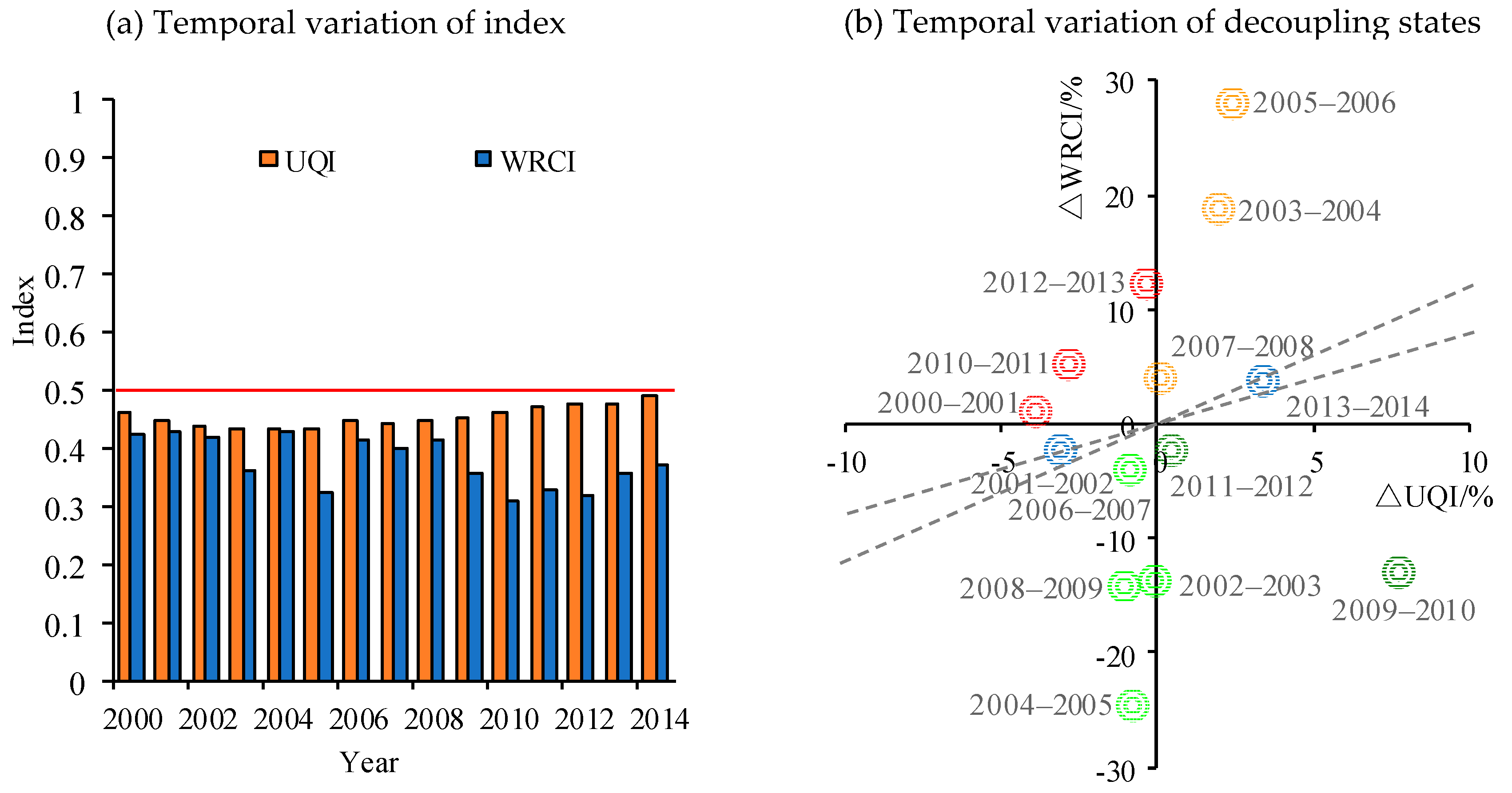
3.1. Temporal Variation of UQI and WRCI of the Whole Northwest China

For the whole Northwest China, UQI and WRCI were both less than 0.5 during 2000–2014 (Figure 3a), belonging to the LL spatial coupling type all along. The UQI increased slowly from 0.4607 in 2000 to 0.4898 in 2014 with a slight fluctuation. According to the grading criterions in Table 2, it belonged to the medium level. The WRCI decreased from 0.4250 in 2000 to 0.3705 in 2014 with a relatively large fluctuation (Figure 3a). According to the grading criterions in Table 2, it belonged to the medium or lower level. It indicates that water resources have less strong constraint or weak constraint on socio-economic development. The whole Northwest China still has some potential to develop its water resources. However, the urbanization quality is not high and still needs to be improved.
Figure 3b shows the decoupling states of the whole Northwest China during every one-year period in 2000–2014. On the whole, as the UQI increased and the WRCI decreased, the decoupling index is −5.05. Northwest China had achieved strong decoupling over the entire period. However, the WRCI showed strong decoupling with UQI only in 2009–2010 and 2011–2012, which was the optimal and coordinated state. Strong negative decoupling appeared in 2000–2001, 2010–2011 and 2012–2013, which was the worst and uncoordinated state. Expansive coupling appeared in 2013–2014. Expansive negative decoupling appeared in 2003–2004, 2005–2006 and 2007–2008. Weak negative decoupling appeared in 2001–2002. Recessive decoupling appeared in 2002–2003, 2004–2005, 2006–2007 and 2008–2009. It indicates that the temporal decoupling relationship between UQI and WRCI in the whole Northwest China was irregular and sensitive. As the changes of UQI and WRCI in the whole Northwest China were influenced by multiple and complicated indicators, integrated and real-time countermeasures should be adopted to coordinate their relationship.

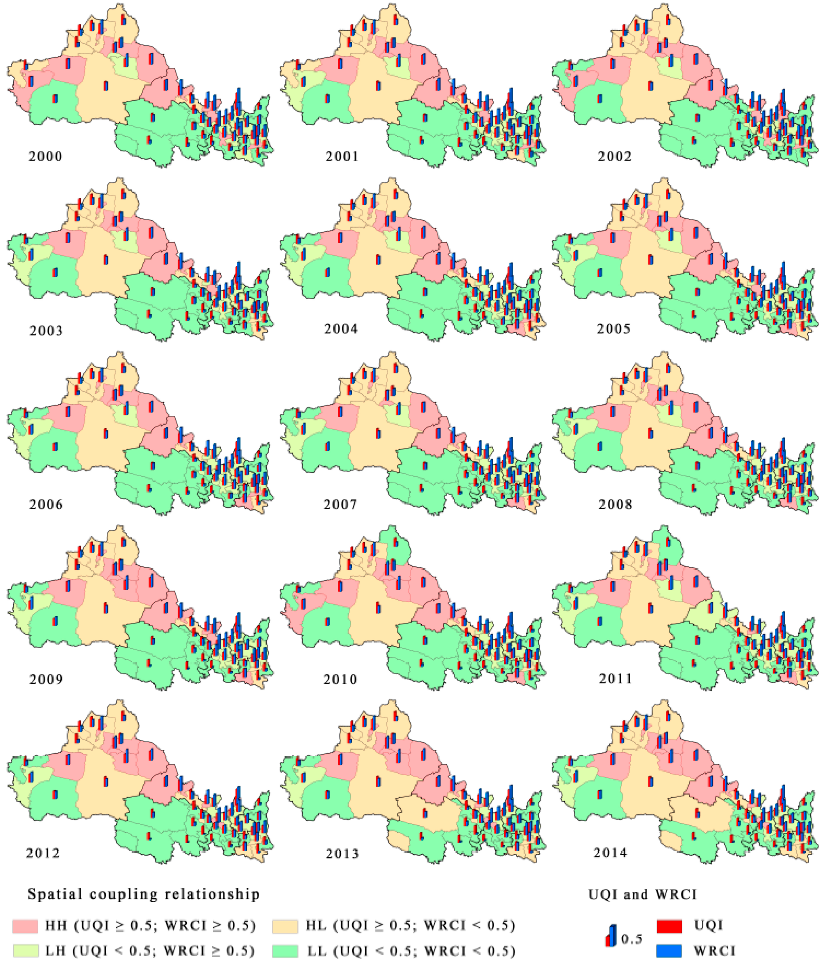
3.2. Spatiotemporal Variation of the Coupling Relationship between UQI and WRCI

Based on the classification method in Table 4, the coupling relationships between UQI and WRCI in 51 prefecture level regions of Northwest China during 2000–2014 are illustrated in Figure 4. Among them, HH-type regions were mainly distributed along the Eurasian Continental Bridge. Most of them were the core areas of urbanization development in Northwest China, while facing serious water resources constraint. The number of HH-type regions decreased from 14 in 2000 to 8 in 2007, and increased to 12 in 2014, with a slight fluctuation.
HL-type regions were centrally distributed in Xinjiang Autonomous Region and scattered in Gansu and Shaanxi Province. They had high urbanization quality and low water resources constraint intensity. The coupling relationship between UQI and WRCI in these regions were optimal and coordinated. They were key development areas of Northwest China. Fortunately, the number of HL-type regions increased from 7 in 2000 to 11 in 2014.
LH-type regions were mainly located in Eastern Gansu, Southern Ningxia and Central Shaanxi. These regions had low urbanization quality and high water resources constraint intensity. The coupling relationship between UQI and WRCI in these regions were the worst and uncoordinated. They were key problem areas of Northwest China. Unfortunately, the number of LH-type regions increased from 13 in 2000 to 21 in 2008, decreased to 9 in 2013 and increased to 13 in 2014.
LL-type regions were centrally distributed in Qinghai and scattered in Gansu, Xinjiang and Shaanxi. Most of them were minority nationality regions. They had good natural endowment of water resources. However, the infrastructures and urbanization processes were lagged. The number of LL-type regions, ranging from 16 to 23, was the largest among all the four kinds of regions in Northwest China.

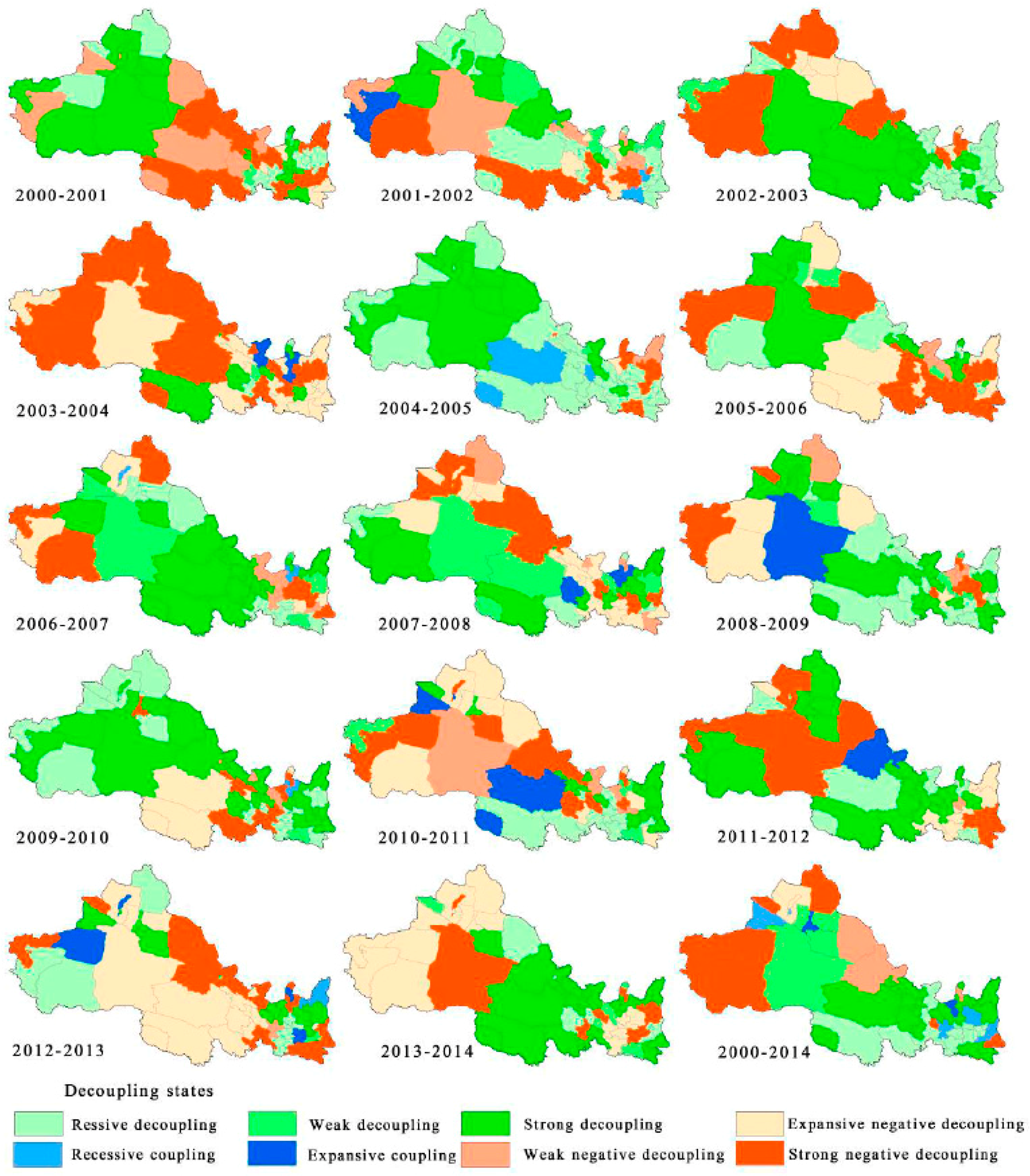
3.3. Spatiotemporal Variation of the Decoupling Relationship between UQI and WRCI

Based on the temporal decoupling classification method, the decoupling relationships between UQI and WRCI in 51 prefecture level regions of Northwest China during 2000–2014 are illustrated in Figure 5.
As shown in Figure 5, during the entire period in 2000–2014, most prefecture level regions in Northwest China belonged to the decoupling type, occupying 60.78% of the total amount. They were widely distributed in the central and southern areas. The negative decoupling type and the coupling type occupied 25.49% and 13.73% respectively. They were scattered in border regions. More specifically, the strong decoupling type widely appeared in Northern Shaanxi, Ningxia, Northern Gansu and Northern Qinghai. The weak decoupling type occurred mainly in Western Xinjiang. The recessive decoupling type mainly occurred in Southern Qinghai and Southern Gansu. The negative decoupling type, mainly in the form of strong negative decoupling, widely occurred in Xinjiang and scattered in Shaanxi, Ningxia and Gansu. In addition, the expansive coupling type and the recessive coupling type were scattered in Northwest China.
From the perspective of every one-year period changes in 2000–2014, Northwest China was confronted with great disparity in the decoupling relationship between UQI and WRCI (Figure 5). On the whole, the decoupling type appeared 369 times, occupying 51.68% of the total amount. The negative decoupling type appeared 321 times, occupying 44.96%. The coupling type appeared 24 times, occupying 3.36%. More specifically, the strong decoupling type, which is the optimal and coordinated state, appeared 198 times and occupied 27.73%. The strong negative decoupling type, which is the worst and uncoordinated state, appeared 168 times and occupied 23.53%. The recessive decoupling type appeared 136 times and occupied 19.05%. The expansive negative decoupling type appeared 116 times and occupied 16.25%. The weak negative decoupling type appeared 37 times and occupied 5.18%. The weak decoupling type appeared 35 times and occupied 4.90%. The expansive coupling type appeared 15 times and occupied 2.10%. The recessive coupling type appeared 9 times and occupied 1.26%. In addition, most prefecture level regions had different decoupling types every one-year (Figure 5).

4. Conclusions

This paper constructed an urbanization quality index (UQI) and a water resources constraint intensity index (WRCI), and provided a method to explore the coupling and decoupling relationships between them from a spatiotemporal perspective. Northwest China was taken as an example to validate it, and the following conclusions and policy implications were obtained:
(1) The coupling relationship between UQI and WRCI in the whole Northwest China during 2000–2014 all belonged to LL-type. They had achieved strong decoupling which was the optimal and coordinated state during the entire period. However, the strong decoupling types only appeared in 2009–2010 and 2011–2012. The relationships were uncoordinated in other years. It implicates that, on the one hand, Northwest China should greatly improve its urbanization quality in rapid urbanization, including urban economic development quality, urban social development quality, urban eco-environmental quality, and urban-rural and regional integration quality; on the other hand, when implementing “The Most Stringent Water Management System” to maintain the “three red lines” of water resources management [74,75], the whole Northwest China should explore its potentiality of water resources to the greatest extent. Only in this way can Northwest China realize the coordinated development of urbanization and water resources.
(2) Northwest China was confronted with great disparity in the coupling and decoupling relationships between UQI and WRCI during 2000–2014. Among them, HL-type regions and strong decoupling type regions, where the relationships were optimal and coordinated, were key development areas. They mainly scattered in Gansu and Shaanxi. LH-type regions and strong negative decoupling type regions, where the relationships were the worst and uncoordinated, were key problem areas. They mainly scattered in Shaanxi, Ningxia and Gansu. Other type regions, which were unsatisfactory due to low UQI, high WRCI, decline of UQI or increase of WRCI, were common problem area. It implicates that Northwest China should formulate different urbanization policies and water policies according to local conditions. Only after we delimit the key development areas and key problem areas by the coupling and decoupling relationships between UQI and WRCI can we formulate the targeted policies and measures.
In further study, based on the spatiotemporal characteristics in this paper, we can find out why the coupling and decoupling relationships between UQI and WRCI changed if we analyzed the changes of all indicators in detail. We can also find out the underlying reasons for a certain prefecture-level administrative units through field investigations. These further studies will be also significant to formulate the targeted policies and measures for the New-Type Urbanization constrained by water resources in Northwest China.

Acknowledgments

This work was supported by the National Natural Science Foundation of China (grant number: 41571156), the Major Projects of the National Natural Science Foundation of China (grant number: 41590844), and the Service Project on the Cultivation and Construction for the Characteristic Research Institute of the Chinese Academy of Sciences (grant number: TSYJS02). Thanks to Weifeng Li who graduated from Massachusettes Institute of Technology in USA and Fan Chen who graduated from University of North Carolina at Chapel Hill in USA for English editing. Gratitude also for the helpful comments received from two anonymous reviewers and the editors.

Author Contributions

Chao Bao conceptualized and designed the study, analyzed the data, and wrote paper with results checking. Jianjun Zou collected the original data, calculated the results and gave review suggestions of the manuscript. All authors read and approved the final manuscript.

Conflicts of Interest

The authors declare no conflict of interest.

References

  1. Vo, P.L. Urbanization and water management in Ho Chi Minh City, Vietnam-issues, challenges and perspectives. GeoJournal 2007, 70, 75–89. [Google Scholar] [CrossRef]
  2. Bao, C.; Fang, C.L. Water resources flows related to urbanization in China: Challenges and perspectives for water management and urban development. Water Resour. Manag. 2012, 26, 531–552. [Google Scholar] [CrossRef]
  3. Martin-Carrasco, F.; Garrote, L.; Iglesias, A.; Mediero, L. Diagnosing causes of water scarcity in complex water resources systems and identifying risk management actions. Water Resour Manag. 2013, 27, 1693–1705. [Google Scholar] [CrossRef] [Green Version]
  4. Peng, J.; Tian, L.; Liu, Y.; Zhao, M.; Hu, Y.; Wu, J. Ecosystem services response to urbanization in metropolitan areas: Thresholds identification. Sci. Total Environ. 2017, 607–608, 706–714. [Google Scholar] [CrossRef] [PubMed]
  5. Chitsaz, N.; Azarnivand, A. Water scarcity management in arid regions based on an extended multiple criteria technique. Water Resour. Manag. 2017, 31, 233–250. [Google Scholar] [CrossRef]
  6. Gleick, P.H. Global freshwater resources: Soft-path solutions for the 21st century. Science 2003, 302, 1524–1528. [Google Scholar] [CrossRef] [PubMed]
  7. Wan, G.H.; Wang, C. Unprecedented urbanization in Asia and its impacts on the environment. Aust. Econ. Rev. 2014, 47, 378–385. [Google Scholar] [CrossRef]
  8. Dos Santos, S.; Adams, E.A.; Neville, G.; Wada, Y.; de Sherbinin, A.; Mullin Bernhardt, E.; Adamo, S.B. Urban growth and water access in sub-Saharan Africa: Progress, challenges, and emerging research directions. Sci. Total Environ. 2017, 607–608, 497–508. [Google Scholar] [CrossRef] [PubMed]
  9. Bao, C.; Fang, C.L. Water resources constraint force on urbanization in water deficient regions: A case study of the Hexi Corridor, arid area of NW China. Ecol. Econ. 2007, 62, 508–517. [Google Scholar] [CrossRef]
  10. Yang, X.J. China’s rapid urbanization. Science 2013, 342. [Google Scholar] [CrossRef] [PubMed]
  11. Fang, C.L.; Bao, C.; Huang, J.C. Management implications to water resources constraint force on socio-economic system in rapid urbanization: A case study of Hexi Corridor, NW China. Water Resour. Manag. 2007, 21, 1613–1633. [Google Scholar] [CrossRef]
  12. Bao, C.; Fang, C.L. Interaction mechanism and control modes on urbanization and water resources exploitation and utilization. Urban Stud. 2010, 17, 19–23. (In Chinese) [Google Scholar]
  13. Fitzhugh, T.W.; Richter, B.D. Quenching urban thirst: Growing cities and their impacts on freshwater ecosystems. Bioscience 2004, 54, 741–754. [Google Scholar] [CrossRef]
  14. Braud, I.; Breil, P.; Thollet, F.; Lagouy, M.; Branger, F.; Jacqueminet, C.; Kermadi, S.; Michel, K. Evidence of the impact of urbanization on the hydrological regime of a medium-sized periurban catchment in France. J. Hydrol. 2013, 485, 5–23. [Google Scholar] [CrossRef] [Green Version]
  15. Bao, C.; Chen, X.J. The driving effects of urbanization on economic growth and water use change in China: A provincial-level analysis in 1997–2011. J. Geogr. Sci. 2015, 25, 530–544. [Google Scholar] [CrossRef]
  16. Jenerette, G.D.; Larsen, L. A global perspective on changing sustainable urban water supplies. Glob. Planet. Chang. 2006, 50, 202–211. [Google Scholar] [CrossRef]
  17. Bao, C.; Fang, C.L. Study on the quantitative relationship between urbanization and water resources utilization in the Hexi Corridor. J. Nat. Resour. 2006, 21, 301–310. (In Chinese) [Google Scholar]
  18. Fang, C.L.; Yu, D.L. China’s New Urbanization: Developmental Paths, Blueprints and Patterns; Science Press: Beijing, China, 2016. [Google Scholar]
  19. Ye, Y.M. Approach on China’s urbanization quality. China Soft Sci. 2001, 7, 27–31. (In Chinese) [Google Scholar]
  20. Fang, C.L.; Wang, D.L. Comprehensive measures and improvement of Chinese urbanization development quality. Geogr. Res. 2011, 30, 1931–1946. (In Chinese) [Google Scholar]
  21. Xu, S.; Yu, T.; Wu, Q. A study of urbanization quality assessment system of county-level cities in China under the regional perspective: Taking the Yangtze delta area as an example. Urban Plan. Int. 2011, 26, 53–58. (In Chinese) [Google Scholar]
  22. Zhang, C.; Zhang, X.; Wu, Q. Measures and improvement of urbanization development quality in the developed area: A case study of Jiangsu. Econ. Geogr. 2012, 32, 50–55. (In Chinese) [Google Scholar]
  23. Liang, Z.; Chen, C.; Liu, J.; Mei, L. Tiers features and comprehensive measures of urbanization development quality of Northeast China. Sci. Geogr. Sin. 2013, 33, 926–934. (In Chinese) [Google Scholar]
  24. Zhou, D.; Xu, J.; Li, W.; Tan, J. Assessing urbanization quality using structure and function analyses: A case study of the urban agglomeration around Hangzhou Bay (UAHB), China. Habitat Int. 2015, 49, 165–176. [Google Scholar] [CrossRef]
  25. Xue, D.S.; Zeng, X.J. Evaluation of China’s urbanization quality and analysis of its spatial pattern transformation based on the modern life index. Acta Geogr. Sin. 2016, 71, 194–204. (In Chinese) [Google Scholar]
  26. Bao, C.; Fang, C.L. Integrated assessment model of water resources constraint intensity on urbanization and its application in arid area. J. Geogr. Sci. 2009, 19, 273–286. [Google Scholar] [CrossRef]
  27. Ding, Y.F.; Tang, D.S.; Dai, H.C.; Wei, Y.H. Human-water harmony index: A new approach to assess the human water relationship. Water Resour. Manag. 2014, 28, 1061–1077. [Google Scholar] [CrossRef]
  28. Gain, A.K.; Giupponi, C. A dynamic assessment of water scarcity risk in the Lower Brahmaputra River Basin: An integrated approach. Ecol. Indic. 2015, 48, 120–131. [Google Scholar] [CrossRef]
  29. Pedro-Monzonís, M.; Solera, A.; Ferrer, J.; Estrela, T.; Paredes-Arquiola, J. A review of water scarcity and drought indexes in water resources planning and management. J. Hydrol. 2015, 527, 482–493. [Google Scholar] [CrossRef]
  30. Falkenmark, M.; Lundqvist, J.; Widstrand, C. Macro-scale water scarcity requires micro-scale approaches. Nat. Res. Forum 1989, 13, 258–267. [Google Scholar] [CrossRef]
  31. European Environment Agency (EEA). The European Environment—State and Outlook 2005; European Environmental Agency: Copenhagen, Denmark, 2005. [Google Scholar]
  32. Vörösmarty, C.J.; Douglas, E.M.; Green, P.A.; Revenga, C. Geospatial indicators of emerging water stress: An application to Africa. AMBIO J. Hum. Environ. 2005, 34, 230–236. [Google Scholar] [CrossRef]
  33. Sullivan, C.A. Calculating a water poverty index. World Dev. 2002, 30, 1195–1210. [Google Scholar] [CrossRef]
  34. Sullivan, C.A.; Meigh, J.R.; Giacomello, A.M.; Steyl, I. The water poverty index: Development and application at the community scale. Nat. Resour. Forum 2003, 27, 189–199. [Google Scholar] [CrossRef]
  35. Jia, S.F.; Zhang, J.Y.; Zhang, S.F. Regional water resources stress and water resources security appraisement indicators. Prog. Geogr. 2002, 21, 538–545. (In Chinese) [Google Scholar]
  36. Liu, M.; Wei, J.H.; Wang, G.Q.; Wang, F. Water resources stress assessment and risk early warning—Case of Hebei Province China. Ecol. Indic. 2017, 73, 358–368. [Google Scholar] [CrossRef]
  37. Zeng, Z.; Liu, J.; Savenije, H. A simple approach to assess water scarcity integrating water quantity and quality. Ecol. Indic. 2013, 34, 441–449. [Google Scholar] [CrossRef]
  38. Liang, Y.; Xu, X.Y.; Wang, H.R.; Pang, B.; Liu, X. Research on the degree of water shortage in Yunnan Province based on circulating correction mode. J. Nat. Resour. 2013, 28, 1146–1158. (In Chinese) [Google Scholar]
  39. Wang, Y.Z.; Shi, G.Q.; Wang, D.S. Study on evaluation indexes of regional water resources carrying capacity. J. Nat. Resour. 2005, 20, 597–604. (In Chinese) [Google Scholar]
  40. Gong, L.; Jin, C.L. Fuzzy comprehensive evaluation for carrying capacity of regional water resources. Water Resour. Manag. 2009, 23, 2505–2513. [Google Scholar] [CrossRef]
  41. Xia, J.; Zhu, Y.Z. The measurement of water resources security: A study and challenge on water resources carrying capacity. J. Nat. Resour. 2002, 17, 5–7. (In Chinese) [Google Scholar]
  42. Jia, X.; Li, C.; Cai, Y.; Wang, X.; Sun, L. An improved method for integrated water security assessment in the Yellow River basin, China. Stoch. Environ. Res. Risk Assess. 2015, 29, 2213–2227. [Google Scholar] [CrossRef]
  43. Huang, J.C.; Fang, C.L. Analysis of coupling mechanism and rules between urbanization and eco-environment. Geogr. Res. 2003, 22, 211–220. (In Chinese) [Google Scholar]
  44. Fang, C.L.; Wang, J. A theoretical analysis of interactive coercing effects between urbanization and eco-environment. Chin. Geogr. Sci. 2013, 23, 147–162. [Google Scholar] [CrossRef]
  45. Li, Y.F.; Li, Y.; Zhou, Y.; Shi, Y.; Zhu, X. Investigation of a coupling model of coordination between urbanization and the environment. J. Environ. Manag. 2012, 98, 127–133. [Google Scholar] [CrossRef] [PubMed]
  46. Wang, S.J.; Ma, H.T.; Zhao, Y.B. Exploring the relationship between urbanization and the eco-environment—A case study of Beijing-Tianjin-Hebei region. Ecol. Indic. 2014, 45, 171–183. [Google Scholar] [CrossRef]
  47. Ding, L.; Zhao, W.T.; Huang, Y.L.; Liu, C. Research on the coupling coordination relationship between urbanization and the air environment: A case study of the area of Wuhan. Atmosphere 2015, 6, 1539–1558. [Google Scholar] [CrossRef]
  48. Zhao, Y.; Wang, S.; Zhou, C. Understanding the relation between urbanization and the eco-environment in China’s Yangtze River Delta using an improved EKC model and coupling analysis. Sci. Total Environ. 2016, 571, 862–875. [Google Scholar] [CrossRef] [PubMed]
  49. He, J.Q.; Wang, S.J.; Liu, Y.Y.; Ma, H.T.; Liu, Q.Q. Examining the relationship between urbanization and the eco-environment using a coupling analysis: Case study of Shanghai, China. Ecol. Indic. 2017, 77, 185–193. [Google Scholar] [CrossRef]
  50. Organization for Economic Cooperation and Development (OECD). Indicators to Measure Decoupling of Environmental Pressure from Economic Growth; OECD Report; Organization for Economic Cooperation and Development: Paris, France, 2002. [Google Scholar]
  51. Zhu, H.; Li, W.; Yu, J.; Sun, W.; Yao, X. An analysis of decoupling relationships of water uses and economic development in the two provinces of Yunnan and Guizhou during the first ten years of implementing the Great Western Development Strategy. Procedia Environ. Sci. 2013, 18, 864–870. [Google Scholar] [CrossRef]
  52. Conrad, E.; Cassar, L.F. Decoupling economic growth and environmental degradation: Reviewing progress to date in the small island state of Malta. Sustainability 2014, 6, 6729–6750. [Google Scholar] [CrossRef]
  53. Yu, Y.; Zhou, L.; Zhou, W.; Ren, H.; Kharrazi, A.; Ma, T.; Zhu, B. Decoupling environmental pressure from economic growth on city level: The case study of Chongqing in China. Ecol. Indic. 2017, 75, 27–35. [Google Scholar] [CrossRef]
  54. Tapio, P. Towards a theory of decoupling: Degrees of decoupling in the EU and the case of road traffic in Finland between 1970 and 2001. J. Transp. Policy 2005, 12, 137–151. [Google Scholar] [CrossRef]
  55. Zhou, X.; Zhang, M.; Zhou, M.; Zhou, M. A comparative study on decoupling relationship and influence factors between China’s regional economic development and industrial energy-related carbon emissions. J. Clean. Prod. 2017, 142, 783–800. [Google Scholar] [CrossRef]
  56. Zhao, X.; Zhang, X.; Li, N.; Shao, S.; Geng, Y. Decoupling economic growth from carbon dioxide emissions in China: A sectoral factor decomposition analysis. J. Clean. Prod. 2017, 142, 3500–3516. [Google Scholar] [CrossRef]
  57. Wang, Y.; Xie, T.; Yang, S. Carbon emission and its decoupling research of transportation in Jiangsu Province. J. Clean. Prod. 2017, 142, 907–914. [Google Scholar] [CrossRef]
  58. Deng, H.; Chen, Y.; Shi, X.; Li, W.; Wang, H.; Zhang, S.; Fang, G. Dynamics of temperature and precipitation extremes and their spatial variation in the arid region of Northwest China. Atmos. Res. 2014, 138, 346–355. [Google Scholar] [CrossRef]
  59. Yang, Y.; Feng, Z.; Huang, H.Q.; Lin, Y. Climate-induced changes in crop water balance during 1960–2001 in Northwest China. Agric. Ecosyst. Environ. 2008, 127, 107–118. [Google Scholar] [CrossRef]
  60. Shi, C.; Zhan, J. An input-utput table based analysis on the virtual water by sectors with the five northwest provinces in China. Phys. Chem. Earth 2015, 79–82, 47–53. [Google Scholar] [CrossRef]
  61. Chen, C. Calculation of various Gini coefficients from different regions in China and analysis using the nonparametric model. J. Quant. Tech. Econ. 2007, 24, 133–142. (In Chinese) [Google Scholar]
  62. Mendoza, G.A.; Prabhu, R. Fuzzy methods for assessing criteria and indicators of sustainable forest management. Ecol. Indic. 2004, 3, 227–236. [Google Scholar] [CrossRef]
  63. Zhu, H.; Lei, G.; Wu, X.; Liu, Q. Urbanization quality evaluation based on early warning indicator system: Deepening of urbanization quality evaluation system in Shandong province. Urban Stud. 2011, 18, 7–12. (In Chinese) [Google Scholar]
  64. Hong, X.J. Acceptable range and security line of Gini coefficient. Stat. Res. 2007, 24, 84–87. (In Chinese) [Google Scholar]
  65. Wu, P.L. A quantificational and comparative analysis on the regional water resource pressure and water scarcity in China. J. Northwest Sci-Tech Univ. Agric. For. 2005, 33, 43–149. (In Chinese) [Google Scholar]
  66. Bao, C.; He, D.M. Spatiotemporal characteristics of water resources exploitation and policy implications in the Beijing-Tianjin-Hebei Urban Agglomeration. Prog. Geogr. 2017, 36, 58–67. (In Chinese) [Google Scholar]
  67. Saaty, T.L. How to make a decision: The analytic hierarchy process. Eur. J. Oper. Res. 1990, 48, 9–26. [Google Scholar] [CrossRef]
  68. Saaty, T.L. Fundamentals of Decision Making and Priority Theory with the Analytic Hierarchy Process; RWS Publications: Pittsburgh, PA, USA, 2000. [Google Scholar]
  69. Saaty, T.L. Decision making with the analytic hierarchy process. Int. J. Serv. Sci. 2008, 1, 83–98. [Google Scholar] [CrossRef]
  70. Ho, W. Integrated analytic hierarchy process and its applications—A literature review. Eur. J. Oper. Res. 2008, 186, 211–228. [Google Scholar] [CrossRef]
  71. Sutadian, A.D.; Muttil, N.; Yilmaz, A.G.; Perera, B.J.C. Using the Analytic Hierarchy Process to identify parameter weights for developing a water quality index. Ecol. Indic. 2017, 75, 220–233. [Google Scholar] [CrossRef]
  72. Fang, C.L.; Mao, H.Y. A system of indicators for regional development planning. Acta Geogr. Sin. 1999, 54, 410–419. (In Chinese) [Google Scholar]
  73. Zhang, Z.X. Decoupling China’s carbon emissions increase from economic growth: An economic analysis and policy implications. World Dev. 2000, 28, 739–752. [Google Scholar] [CrossRef]
  74. Zang, Z.; Zou, X.; Xi, X.; Zhang, Y.; Zheng, D.F.; Sun, C.Z. Quantitative characterization and comprehensive evaluation of regional water resources using the Three Red Lines method. J. Geogr. Sci. 2016, 26, 397–414. [Google Scholar] [CrossRef]
  75. Ge, M.; Wu, F.; Chen, X. A coupled allocation for regional initial water rights in Dalinghe Basin, China. Sustainability 2017, 9, 428–443. [Google Scholar] [CrossRef]
Figure 1. Location and 51 prefecture level regions of Northwest China.
Sustainability 09 01960 g001
Figure 2. Framework for decoupling judgments on UQI and WRCI based on the Tapio decoupling indicator.
Sustainability 09 01960 g002
Figure 3. Temporal variation of UQI and WRCI of the whole Northwest China in 2000–2014. (a) Temporal variation of index; (b) Temporal variation of decoupling states.
Sustainability 09 01960 g003
Figure 4. Spatiotemporal variation of the coupling relationship between UQI and WRCI in Northwest China.
Sustainability 09 01960 g004
Figure 5. Spatiotemporal variation of the decoupling relationship between UQI and WRCI in Northwest China.
Sustainability 09 01960 g005
Table 1. Comprehensive indicator system to evaluate urbanization quality index (UQI) and water resources constraint intensity index (WRCI).
TargetPrimary IndicatorsSecondary Indicators
UQIUrban economic development quality (0.2986)Per capita GDP (0.2052)
Ratio of tertiary industry value added to GDP (0.2596)
GDP per unit of total fixed asset investment (0.2638)
GDP per unit of land area (0.2714)
Urban social development quality (0.1762)Per capita urban road area (0.2301)
Per capita mobile phone number (0.2301)
Ratio of R&D expenditure to GDP (0.1877)
Ratio of education expenditure to fiscal expenditure (0.1790)
Medical beds per 10,000 persons (0.1730)
Urban eco-environmental quality (0.2132)Green coverage rate of built-up area (0.3229)
Excellent rate of urban air quality (0.2426)
Wastewater discharge per unit of land area (0.2172)
Waste gas emission per unit of land area (0.2172)
Rural-urban and regional integration quality (0.3120)Urban-rural income gap (0.4481)
Urban-rural labor productivity gap (0.2924)
Regional disparity of economic development (0.2595)
WRCINatural endowment of water resources (0.4830)Per capita water resources (0.5000)
Water resources converted into the depth of surface runoff (0.5000)
Exploitation and utilization degree of water resources (0.3010)Water resources utilization ratio (0.4481)
Surface water resources exploitation ratio (0.2595)
Groundwater resources exploitation ratio (0.2924)
Exploitation and utilization efficiency of water resources (0.2160)Water utilization per unit of GDP (0.3697)
Water utilization per unit of agricultural value-added (0.2058)
Water utilization per unit of industrial value-added (0.2163)
Per capita domestic water consumption (0.2081)
Notes: Numbers in brackets are the weights of each indicator compared with the above hierarchy.
Table 2. Grading criterions and threshold values of the evaluation indicators for UQI and WRCI.
Type or Level   Low   Lower Medium Higher  High
UQI and its primary indicators00.20.40.60.81
Per capita GDP (104 yuan) 00.81.62.43.24.5
Ratio of tertiary industry value-added to GDP (%) 01530456075
GDP per unit of total fixed asset investment 00.61.21.82.43
GDP per unit of land area (104 yuan/km2) 0502003505001500
Per capita urban road area (m2) 0510152025
Per capita mobile phone number 00.30.511.52
Ratio of R&D expenditure to GDP (%) 00.511.522.5
Ratio of education expenditure to fiscal expenditure (%) 0612182430
Medical beds per 10,000 persons 020406080100
Green coverage rate of built-up area (%) 01525354555
Excellent rate of urban air quality (%) 060708090100
Wastewater discharge per unit of land area (104 t/km2) 53210.50
Waste gas emission per unit of land area (108 m3/km2) 2510630.50
Urban-rural income gap ② ④4.843.22.41.61.2
Urban-rural labor productivity gap 209.67.24.82.41
Regional disparity of economic development 10.50.40.30.20
WRCI00.20.40.60.81
Natural endowment of water resources10.80.60.40.20
Exploitation and utilization degree of water resources00.20.40.60.81
Exploitation and utilization efficiency of water resources10.80.60.40.20
Per capita water resources (m3) 30002200170010005000
Water resources converted into the depth of surface runoff (mm) 20015010070400
Water resources utilization ratio (%) 0204070100150
Surface water resources exploitation ratio (%) 020406080100
Groundwater resources exploitation ratio (%) 020406080100
Water utilization per unit of GDP (m3/104 yuan) 0250500100015002000
Water utilization per unit of agricultural value-added (m3/104 yuan) 050010002000500010,000
Water utilization per unit of industrial value-added (m3/104 yuan) 0501002005001000
Per capita domestic water consumption (m3) 020406080100
Notes: Reference: [25]; Reference: [20]; According to the experience of developed countries and regions; Reference: [63]; Reference: [21]; Reference: [64]; Reference: [29,30,35]; Reference: [65,66]; Reference: [29,31,32,35].
Table 3. Values of random index (RI).
n123456789
RI0.000.000.580.961.121.241.321.411.45
Table 4. Classification standard of spatial coupling relationship between UQI and WRCI.
TypeExplanation
HHUQI ≥ 0.5, WRCI ≥ 0.5; a uncoordinated relationship and a common problem area with high water stress
HLUQI ≥ 0.5, WRCI < 0.5; a coordinated relationship and a key development area
LHUQI < 0.5, WRCI ≥ 0.5; a very uncoordinated relationship and a key problem area
LLUQI < 0.5, WRCI < 0.5; a uncoordinated relationship and a common problem area with low UQI

