1. Introduction
Many loads consume less energy when operated at a lower voltage. Not all loads exhibit this behavior, but often an aggregate load, such as the load on a distribution feeder, will consume less energy when operated at a lower voltage [
1,
2]. Lowering voltage to reduce the energy consumed by the aggregate load of a feeder is referred to as conservation voltage reduction, or CVR. The CVR factor for this work is defined as the percentage power flow change that occurs when the supply voltage is lowered by 1%.
The ability to accurately estimate the energy saving of CVR versus its cost, and to evaluate control strategies for implementing CVR, depend upon having load models that reflect the real-world, voltage dependency of the aggregate load [
3]. Developing such models requires field experiments involving changing the voltage magnitude and measuring the change in load. When voltage control devices exist in a substation, they may be used to raise and lower the voltage in a series of experiments to measure load-voltage dependency.
When measuring the effects that voltage changes have on energy consumption, instrumentation often exists for just measuring voltage and current magnitudes, and not for accurately measuring power flows. Such instrumentation can be used to measure the change in current magnitude relative to a change in voltage magnitude, referred to here as the load-voltage dependency factor. The load-voltage dependency factor may be related to other load models, such as loads modeled as a combination of constant power, constant impedance, and constant current.
The load models that are used in power system analysis usually consist of constant impedance and constant power loads. In reality these types of loads do not behave the same with respect to voltage on the system [
4]. In this paper this load-voltage dependency is taken into account and its effect on a coordinated control algorithm is investigated.
There are two main types of control in literature, local and coordinated [
5,
6]. Local controllers include time-controlled capacitors and voltage-controlled capacitors. With technological development, decisions can be made by coordinated control where measurements and model information are used to decide optimum settings for local controllers. Local controllers for switched capacitors, voltage regulators and load tap changers use voltage set points which specify a range for control; the coordinated controller would update the voltage set-points [
7,
8].
Controllable devices include switched capacitor banks, voltage regulators, load tab changers (LTC) and distributed energy resources (DER) [
9,
10]. The set points determined by the coordinated controller will, for instance, coordinate a capacitor bank’s operation with other controllable devices on the feeder. The set points to the switched capacitor may change due to a number of conditions such as growth in loading level, reconfiguration of the feeder, and based on different type of loads and their voltage sensitivity.
In the literature a number of papers have been written to explain the effects of coordinated control on power systems. Abdel Salam, T.S. et al. [
7] describes an algorithm for optimal capacitor placement based on determining nodes whose voltages affect losses in the system the most, but load-voltage dependency factors are not considered. Authors in [
11] propose the coordinated control algorithm with two modes; efficiency and CVR, but the authors assumed a load-voltage dependency factor [
12] uses coordinated control for reduction of losses and to reduce controller motion, again without considering load-voltage dependency. In [
13] the author proposes a coordinated control algorithm to achieve better voltage and operation times of LTC and switched capacitors, but again did not consider load-voltage dependency [
14] explores a coordinated control method for load tab changer and switching capacitor to reduce the operation of both devices without considering different types of loads.
The work here focuses on a new coordinated control algorithm and uses field measurements of load-voltage dependency factors. Approximately 1200 feeders are evaluated for CVR performance, where 11 feeders were selected for being top CVR performers and used in a pilot study. The feeders considered are divided into two types, short feeders, such as those commonly occurring in urban areas, and longer feeders, such as those commonly occurring in rural areas.
This paper is organized as follows: the load-voltage dependency factor is discussed in
Section 2; the coordinated control algorithm is introduced in
Section 3; a case study and a discussion of the results are provided in
Section 4; and, finally, conclusions are given in
Section 5.
2. Load-Voltage Dependency Factor
Load-voltage dependency here relates percent changes in voltages to percent changes in currents. This representation of load-voltage dependency can be calculated using existing measurements of current magnitude and substation voltage magnitude, which are measurements that exist for many distribution feeders that are instrumented.
Table 1 shows some representative load-voltage dependency factors.
From
Table 1 it may be noted that, for common loads, there can be a significant difference between the load-voltage dependencies. However, many distribution feeders have instrumentation that may be used to determine the load-voltage dependency factor, but are not instrumented so that changes in power may be accurately determined. For many existing feeders, measurement of load-voltage dependency at the start of a feeder may be made using existing instrumentation by running many experiments, where the voltage magnitude at the start of the feeder is stepped up and down, and the change in current magnitude is measured. Since load-voltage dependency factors vary with the load mixture, these experiments can be run at different times, such as during the summer and during the winter, to determine time varying values to use for the load-voltage dependency.
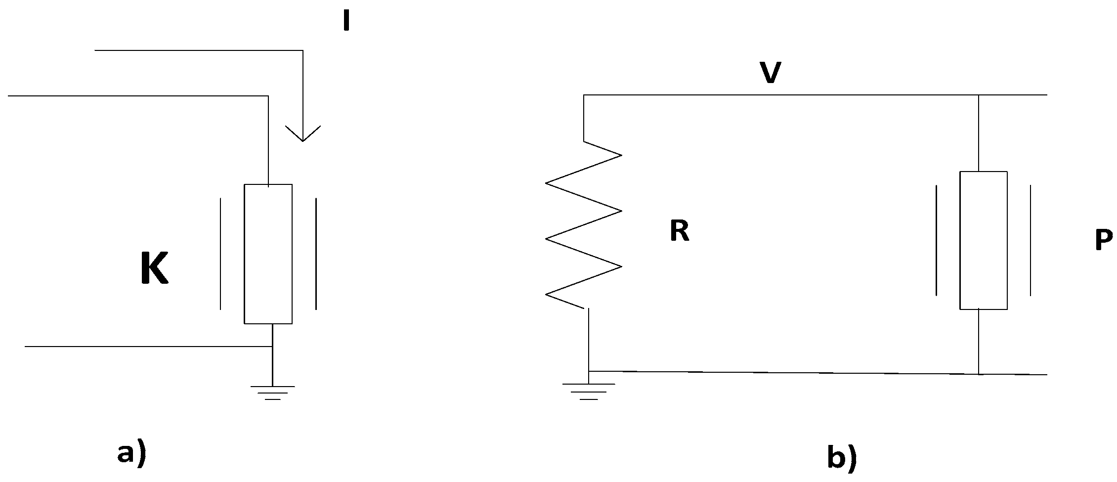
The relation between the load-voltage dependency factors for constant impedance and constant power load models will now be considered and is shown
Figure 1.
Equation (1) relates the load-voltage dependency model; the right hand side of Equation (1), to a load model consisting of constant power and constant impedance, while the left hand side of Equation (1) is the load-voltage dependency model:
where
= fraction of load that is constant power; V = actual voltage magnitude; I = actual current magnitude;
= nominal voltage magnitude;
= nominal current;
R = constant impedance =
;
= constant power load;
= constant impedance load; and V × I = voltage dependent load. Substituting
and I =
into Equation (1) gives:
where
K = load−voltage dependency where:
If K = 1, then the load becomes a constant impedance load when K = 0, the load becomes a constant current load. When K = −1 the load becomes a constant power load.
Let the actual voltage be related to the nominal voltage by:
Substituting Equation (3) into Equation (2), we obtain
K as a function of
h and
f, as given by:
Applying L’Hospital’s rule to Equation (4) for
h = 1, we get:
Given an experimentally-measured value of
K and a value of
h, Equations (4) and (5) may be used to determine the value of
.
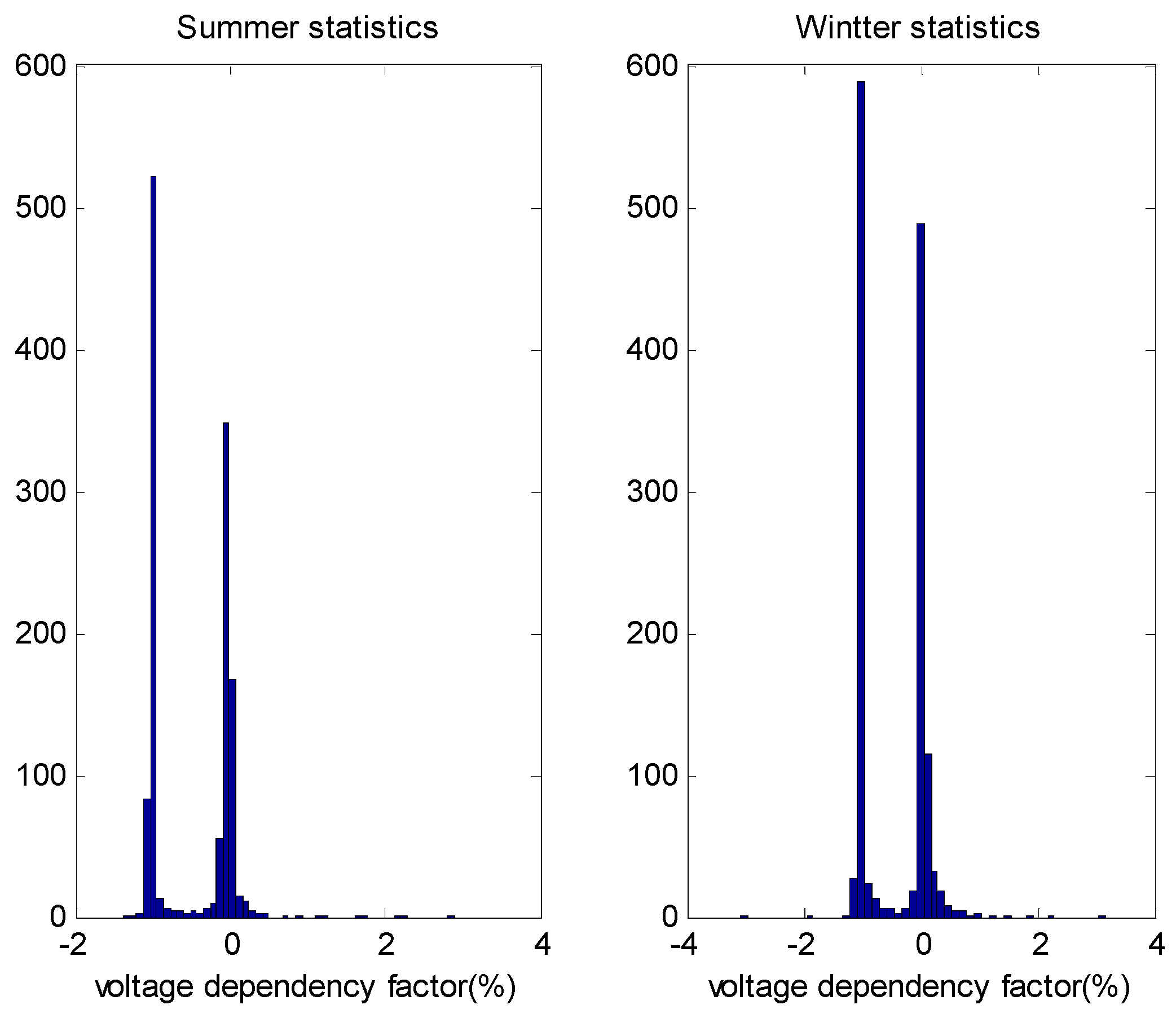
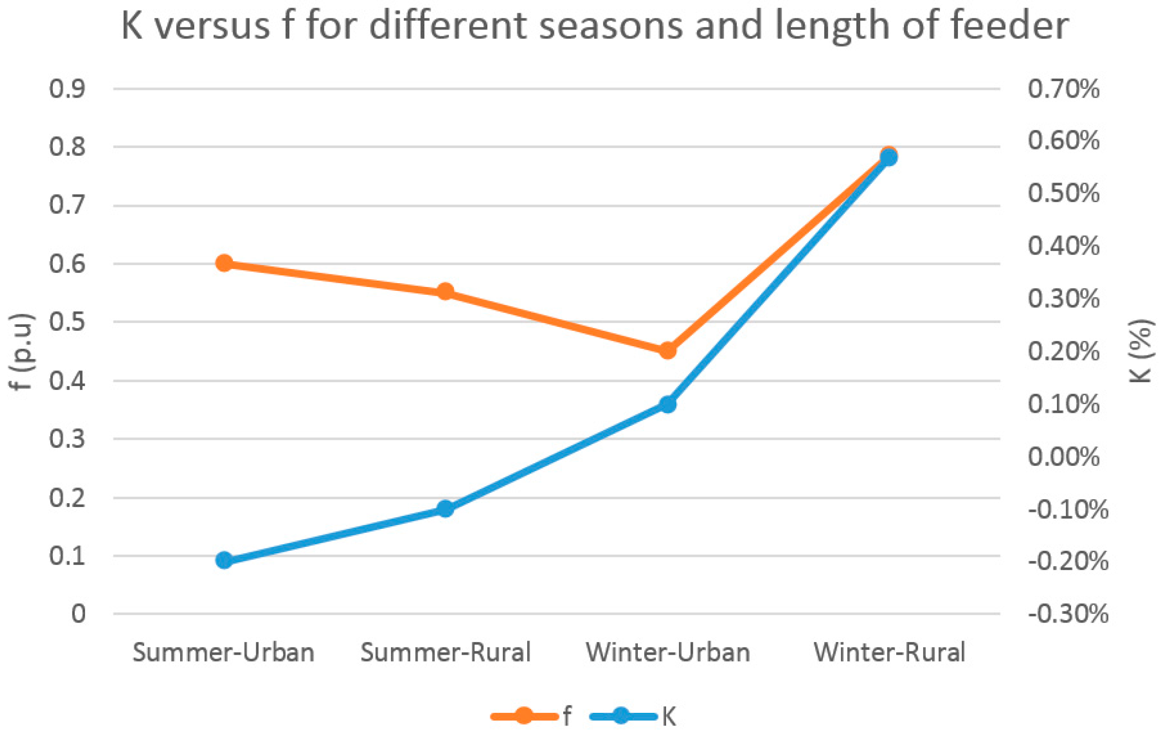
values associated with
K values for different seasons and length of feeders are measured and plotted in
Figure 2.
Figure 2 illustrates how the load-voltage dependency factor can vary with seasons and length of the feeder. The feeders are divided into two types based on length, where short feeders are less than 5 miles long and long feeders are more than 5 miles. Short feeders consist of 60% constant power (40% constant impedance) during the summer, while during the winter the same feeders behave with 45% constant power (55% constant impedance). The long feeders operate with 55% constant power load during the summer and 80% constant power load during the winter.
3. Coordinated Control Algorithm
The coordinated control algorithm serves here for minimizing energy delivered by reducing voltage while maintaining the voltage within an acceptable range.
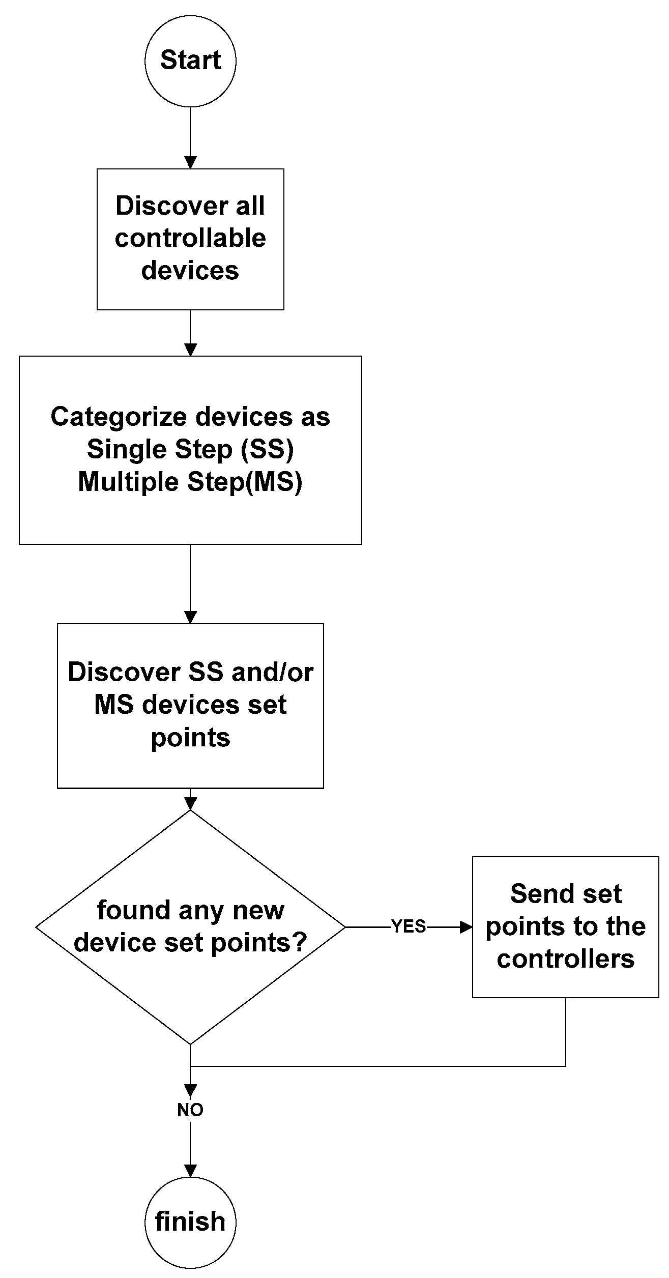
The control algorithm first discovers all the controllable devices—switchable capacitors, voltage regulators, load tap changers—in feeders. Additionally, the coordinated control algorithm automatically discovers control devices when they inserted or removed. In addition to this discovery, the coordinated control also categorizes the control devices as single step or multiple step and determines optimum set points for the local controllers. Single step devices in this study are switched capacitors since it has just ON or OFF mode. Voltage regulators and load tap changers are multi-step control devices, since they have a 16 step size in this study and, based on the required voltage algorithm, decides which steps are the best choice for voltage interval.
Figure 3 shows how the discovery process of coordinated control works. This discovery needs to run before the coordinated control runs since the coordinated control needs to know all controllable devices and to categorize the control devices.
To be able to reach its objective, the coordinated control tries to minimize the customer voltage while maintaining the customer voltage within the required operating range.
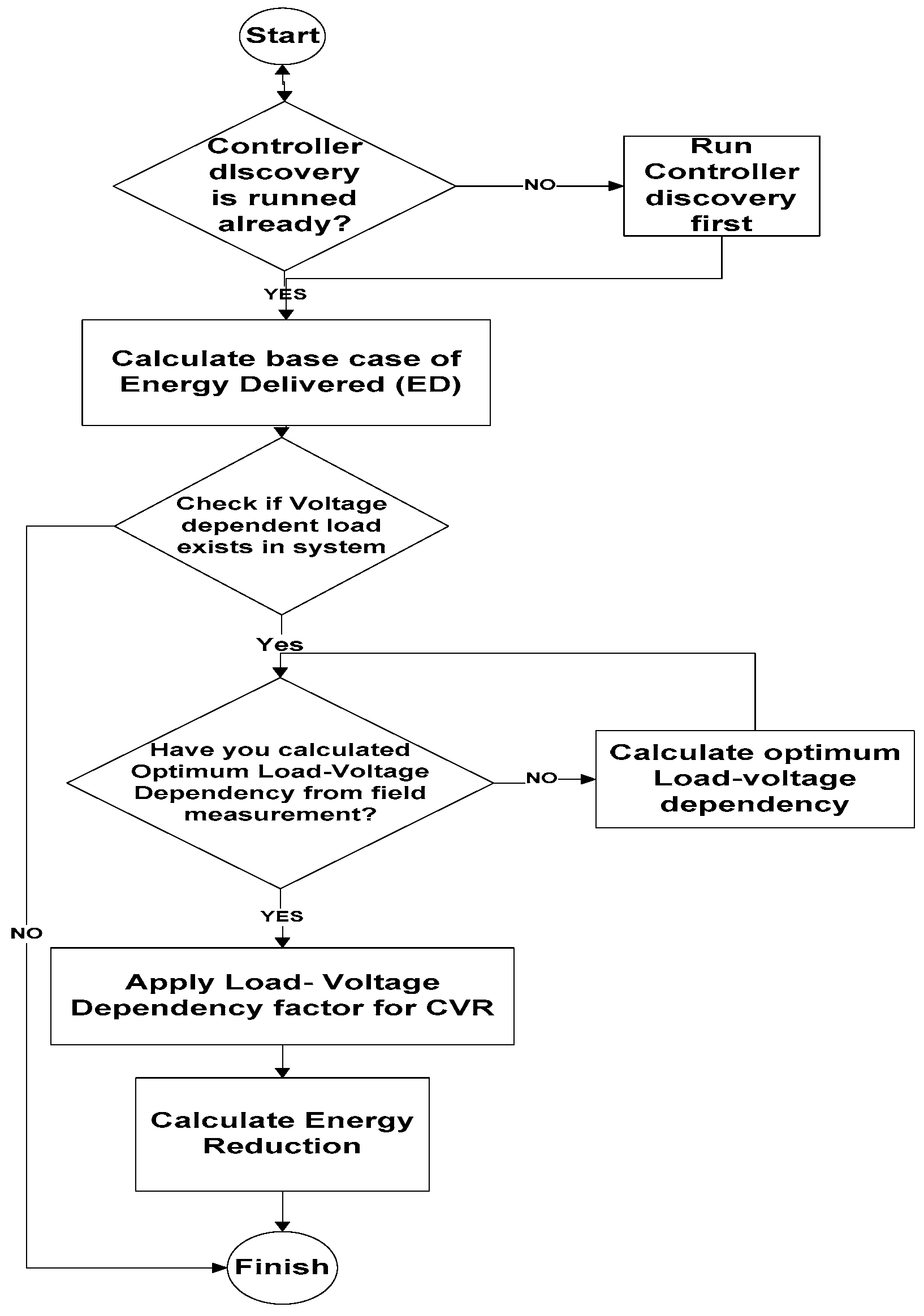
Figure 4 shows the coordinated control algorithm and illustrates the use of load-voltage dependency factors in the energy reduction calculation.
The steps in the algorithm are as follows:
Step 1: Coordinated control runs the discovery algorithm first from
Figure 3 to know the status of control devices and categorizes the control devices.
Step 2: The existing system can be classified as a base case, and then initial voltages and energy delivered are calculated for the base case.
Step 3: Check whether or not load-voltage dependency exists, and exit if there is no load-voltage dependency.
Step 4: If a voltage-dependent load exists, then use the value from field measurements.
Step 5: Coordinated control applies load-voltage dependency factors to estimate the energy reduction achieved.
Step 6: When the iteration has finished, the coordinated control uses the solution as the starting solution for the next iteration.
Step 7: When the algorithm has finished, the optimum local control set points for minimizing the load energy, while maintaining the voltage within the required limits, have been determined.
4. Case Study: CVR and Energy Results
In this section results from a CVR study on a system consisting of more than 1200 feeders is presented.
4.1. Results for the Entire System
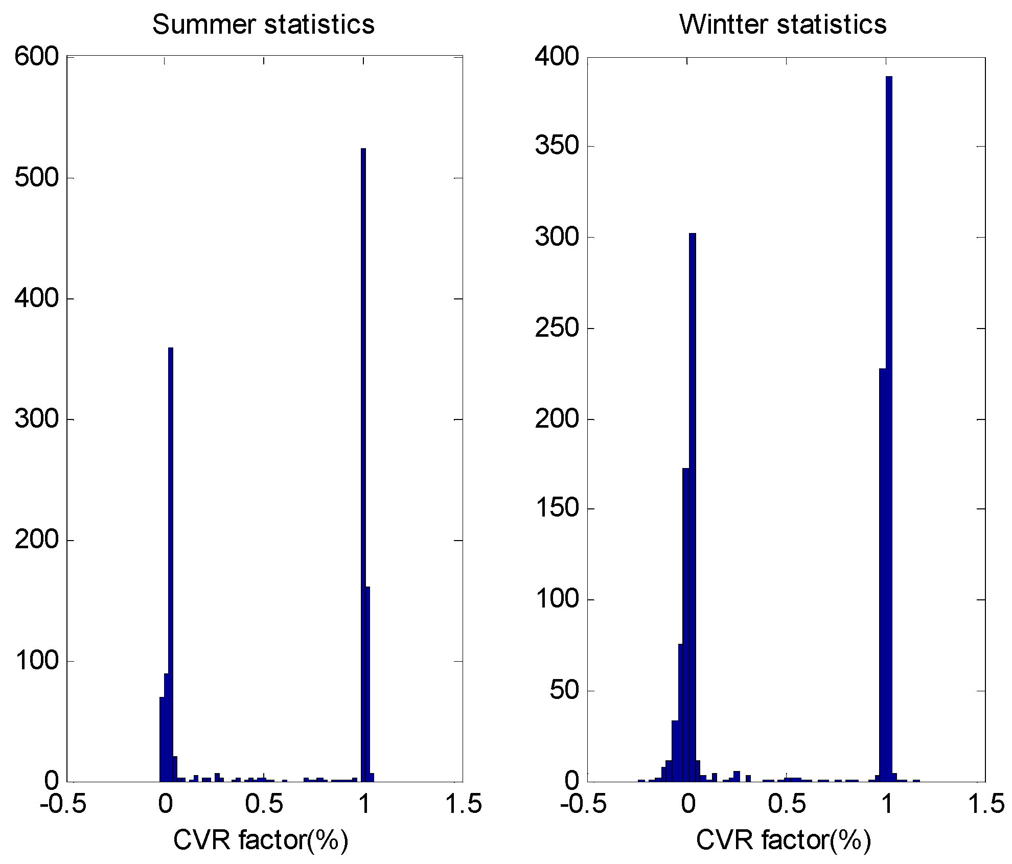
Statistical variations in load-voltage dependency factors and CVR factors for different seasons are shown in
Figure 5 and
Figure 6. The reason the load-voltage dependency and CVR factors varying for different seasons is the change in types of loads used in different seasons.
Implementing CVR with coordinated control versus implementing CVR with local control is compared next. From
Figure 7,
Figure 8,
Figure 9 and
Figure 10 it may be seen that the load energy is significantly lower with coordinated control. In
Figure 7,
Figure 8,
Figure 9 and
Figure 10 only feeders that have an energy savings more than 1% with CVR are considered, which amounted to 260 feeders.
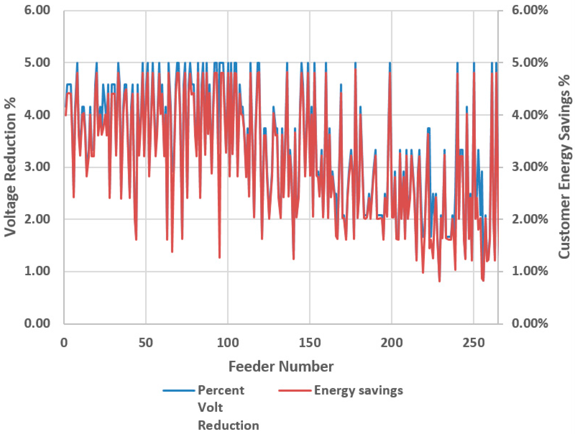
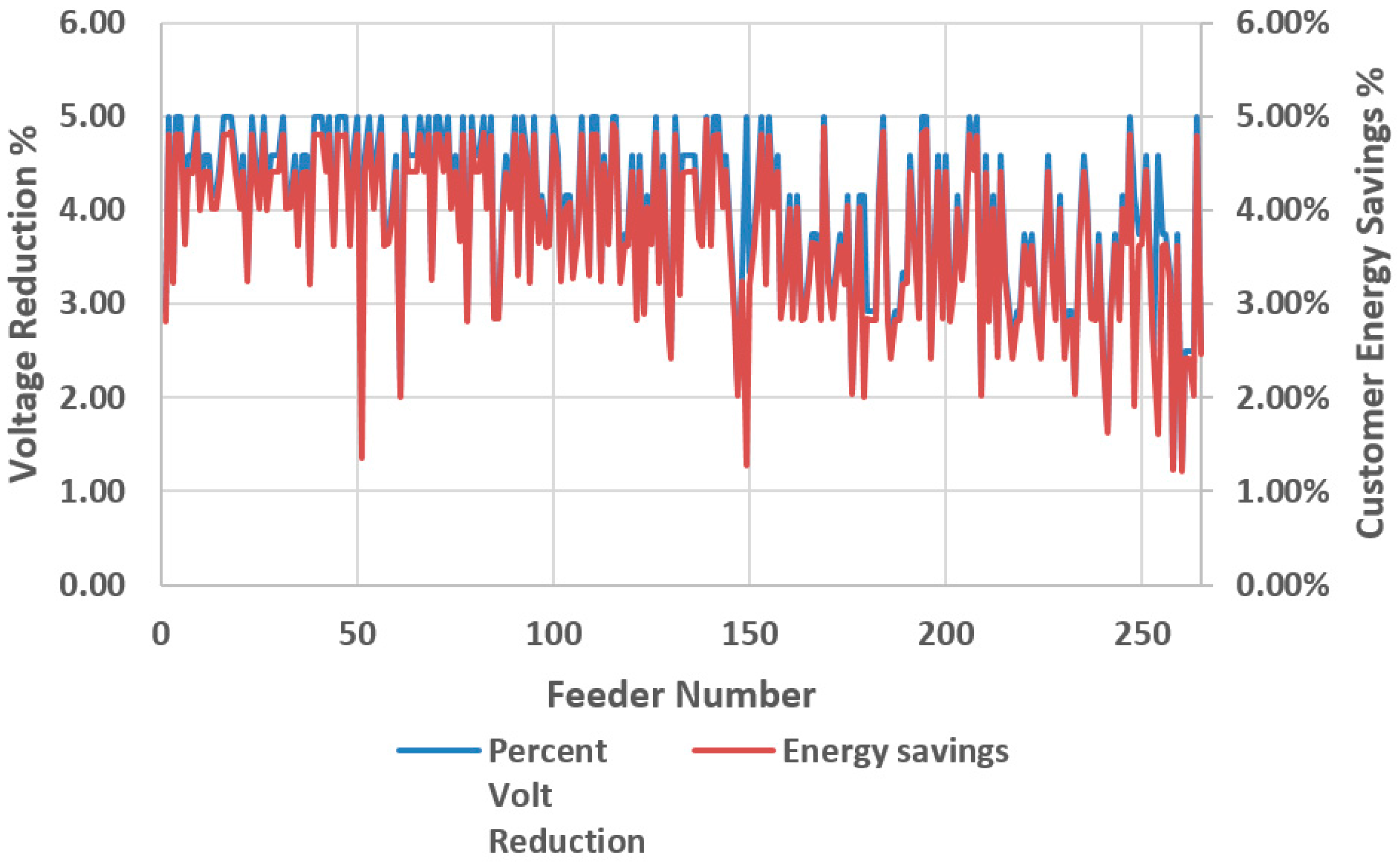
Figure 7,
Figure 8,
Figure 9 and
Figure 10 show the percent energy savings with respect to percent voltage reduction. In
Figure 7 summer savings are illustrated for the urban area’s feeders while
Figure 8 shows winter savings for the urban area’s feeders. For urban area’s feeders during the summer the load-voltage dependency factor is −0.2%, which means the system consists of 60% constant power load and 40% constant impedance load. Average customer energy savings for the urban area’s feeders during the summer is around 2.5%.
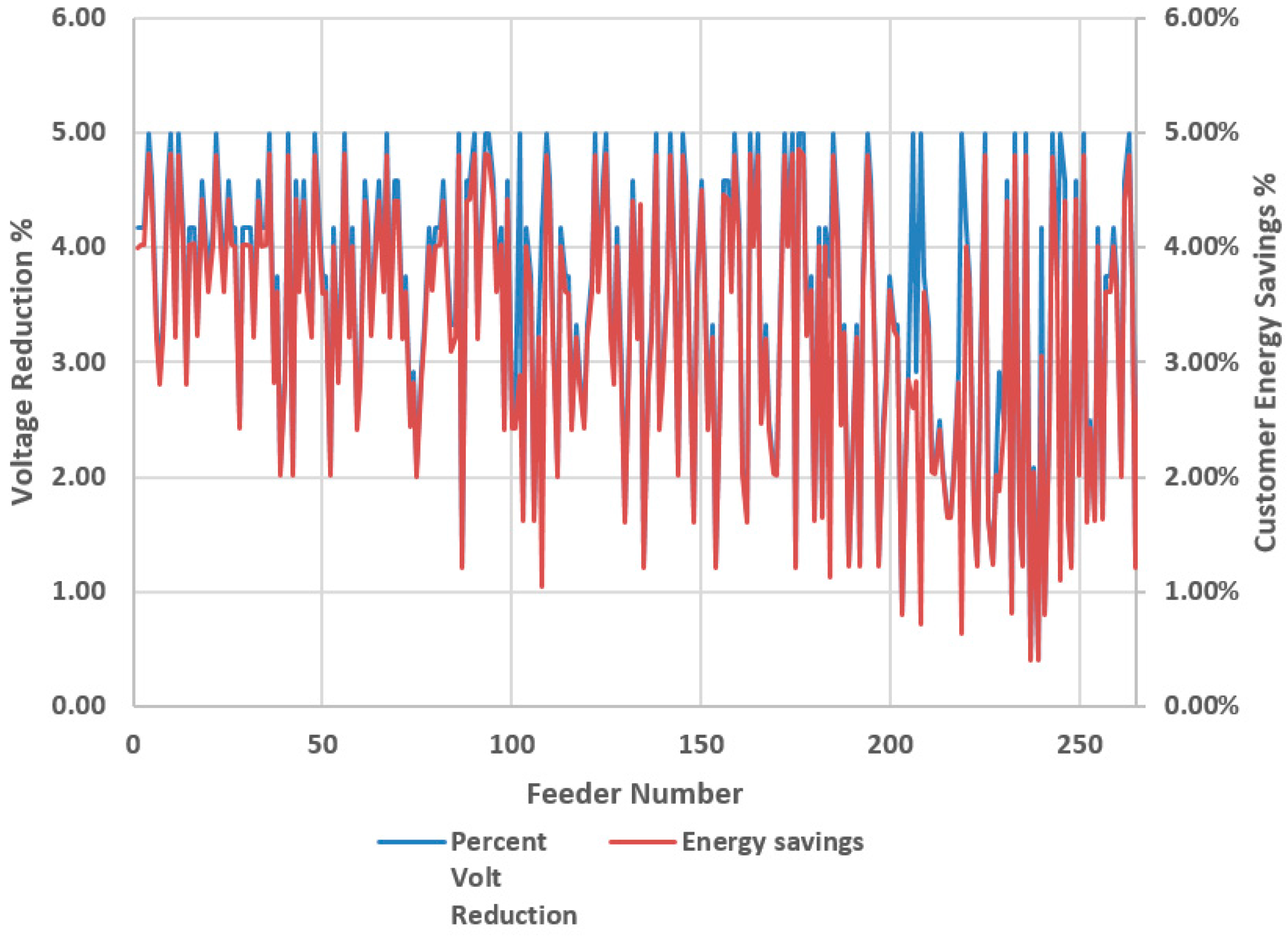
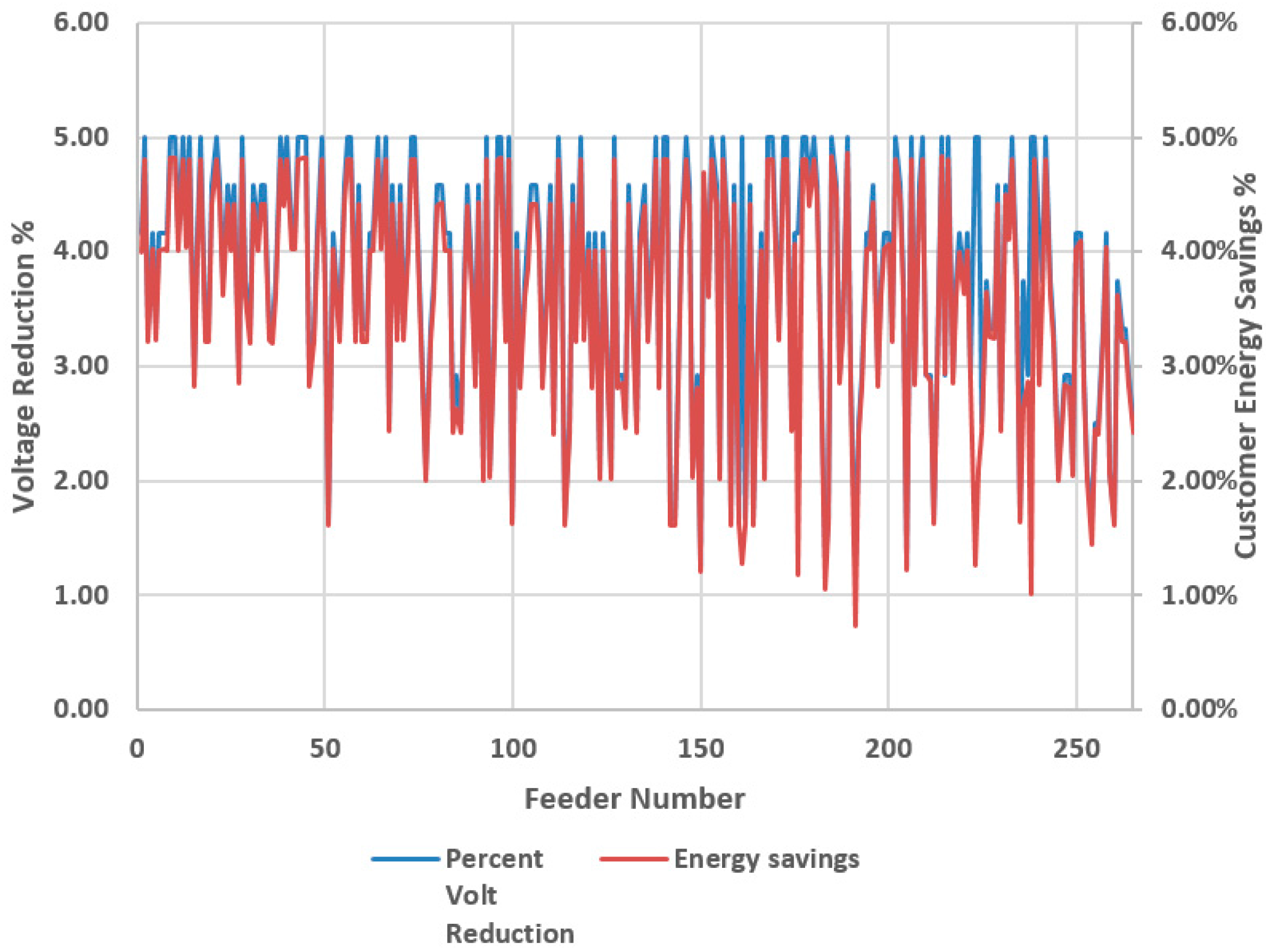
Figure 8 looks at the urban area’s feeders during the winter time where the load-voltage dependency factor is 0.1%, which means the system consists of 45% constant power load and 55% constant impedance load. Average customer energy savings for urban area’s feeders during the winter time is around 3.3%.
Figure 9 looks at the rural area’s feeders during the summer, where the load-voltage dependency factor is around 0.1%, which means that the system consists of 55% constant power load and 45% constant impedance load. The average customer energy savings for rural area’s feeders during the summer time is around 2.8%.
In
Figure 10 the rural area’s feeders during the winter are considered, where the load-voltage dependency factor is 0.57%, which means that the system consists of 78.5% constant power load and 11.5% constant impedance load. The average customer energy savings for rural area’s feeder during the winter is around 3%.
4.2. Results for 11 Feeders
Of the 260 feeders considered in
Section 4.1, the 11 feeders that had the best CVR performance were identified. It should be noted that these top performing feeders all had a relatively flat voltage profile.
Table 2 shows the load-voltage dependency factors for these feeders for the different seasons. As can see from the table, during the summer the load-voltage dependency factors are higher than during the winter.
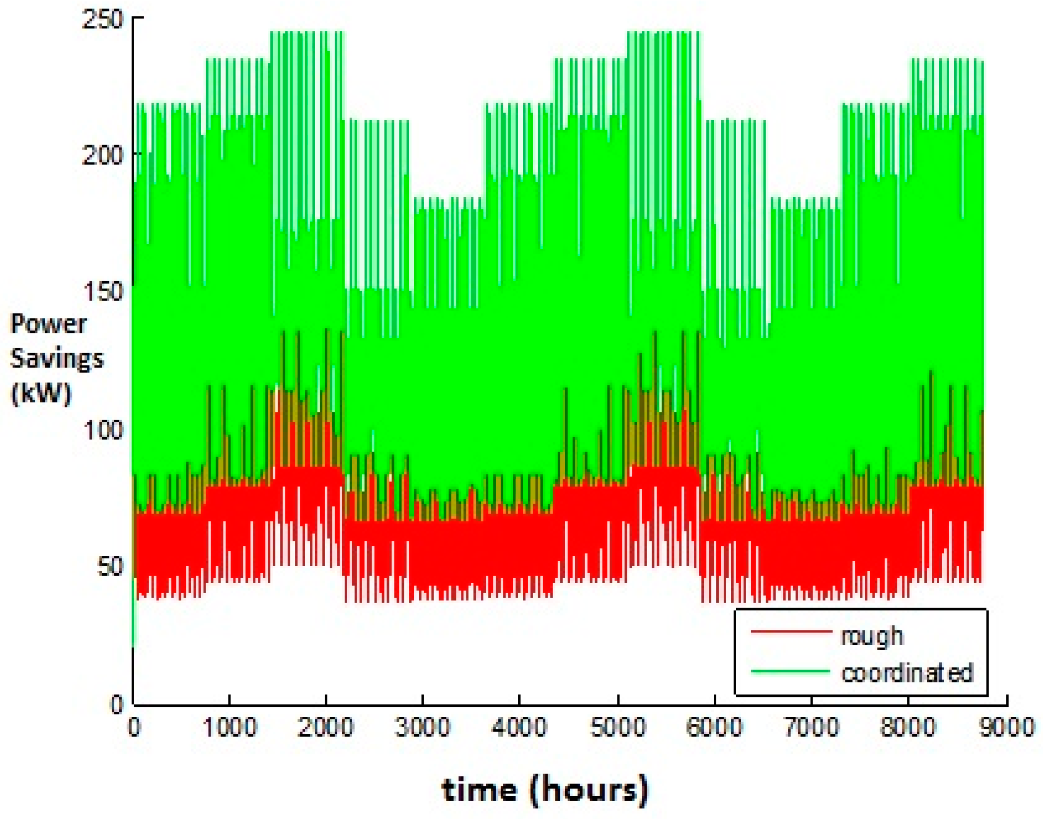
Using the load-voltage dependency factors, the coordinated control was used to analyze the 11 feeders every hour for an entire year (8760 time points).
Figure 11 compares the power savings of coordinated control with the power savings of local control.
Based on the
Figure 11, savings from the coordinated control is 2–3 times greater (around 10 GWhr) than the local control savings. The savings change throughout the year is based on demand. It is interesting to note that the larger the demand, the greater the savings.
5. Conclusions
Load-voltage dependency factors can be measured experimentally on many feeders with existing measurement devices. With respect to load-voltage dependency factors, load combinations were determined which were equivalent to the load-voltage dependency factors. A new coordinated control algorithm that made use of load-voltage dependency factors was described.
Two models were compared based on the reduction of energy. The first model involved feeders with local control and the second model involved feeders with coordinated control. The results showed that coordinated control with conversation voltage reduction helps to reduce the energy delivered. Results presented provide information about energy reduction for different load-voltage dependency factors. Across the two model comparisons of minimizing energy consumption, the coordinated control for conversation voltage reduction showed significant energy reduction over local control.


