Estimation of Distribution Algorithm for Energy-Efficient Scheduling in Turning Processes

Abstract

With the increasing concern for the environment, energy-efficient scheduling of the manufacturing industry is becoming urgent and popular. In turning processes, both spindle speed and processing time affect the final energy consumption and thus the spindle speed and scheduling scheme need to be optimized simultaneously. Since the turning workshop can be regarded as the flexible flow shop, this paper formulates a mixed integer nonlinear programming model for the energy-efficient scheduling of the flexible flow shop. Accordingly, a new decoding method is developed for the optimization of both spindle speed and scheduling scheme simultaneously, and an estimation of the distribution algorithm adopting the new decoding method is proposed to solve large-size problems. The parameters of this algorithm are determined by statistics from a simplified practical case. Validation results of the proposed method show that the makespan is shortened to a large extent, and the consumed energy is significantly saved. These results demonstrate the effectiveness of the proposed mathematical model and algorithm.

1. Introduction

With the increasing attention on global warming and climate change, energy-efficient scheduling is becoming an important objective in the process of production [1]. Since about one-half of energy consumption is industrial [2], the reduction of the energy consumption in the manufacturing process is a global concern. Two methods are often used to reduce energy consumption: developing power-efficient machines [3,4] and designing energy-saving manufacturing system frameworks [5,6]. After long-term endeavors, the first method has maintained a good momentum on the single equipment with manufacturing process improvement, material savings, and waste reduction [7,8,9]. As for the second method, energy-saving through optimization the manufacturing system faces great challenges due to changeable market demand, diversified product structure, and flexible processing routes [10,11,12], as well as insufficient accurate data of energy consumption [13,14], so researchers still struggle to break down these technical and theoretical barriers.

With respect to the energy-efficient scheduling, the well-known machine turn-on and turn-off scheduling framework has been proposed by Mouzon et al. [15] and further explored by Mouzon and Yildirim [16]. Then Dai et al. [17] applied this framework to the flexible flow shop scheduling problem, and Tang et al. [18] adopted it to solve an energy-efficient dynamic scheduling. Since some machines and appliances cannot be switched off during the manufacturing process in some workshops [19], a new method of speed scaling framework has been developed by Fang et al. [20]. Under this framework, Fang et al. [20] researched a flow shop scheduling problem with a restriction on peak power consumption, and Liu and Huang [21] studied a batch-processing machine scheduling problem and a hybrid flow shop problem.

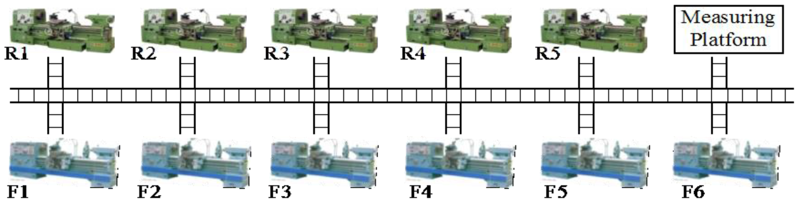
The turning workshop typically involves two processes, i.e., rough turning and fine turning, and each process usually can be completed at any one of parallel lathes, and thus the ordinary turning workshop can be regarded as the flexible flow shop. Salvador [22] originally has proposed the flexible flow shop scheduling problem (FFSP) in oil industry, and this problem is also known as hybrid flow shop scheduling problem (HFSP) [23]. For traditional optimization of the flexible flow shop scheduling, Linn and Zhang [24] pointed out that HFSP is a non-deterministic polynomial (NP) problem after they reviewed computational complexities, scheduling objectives, and solving methods. Aiming at solving the NP problem, Kis and Pesch [25] put forward a method to determine the lower bounds, and they also developed a new branch and bound method which is faster than the method of Azizoglu et al. [26]. However, for large-scale scheduling problems, these optimal methods are inefficient due to high demand for computational time and storage space. Therefore, a lot of heuristics and meta-heuristics were put forward, such as the NEH algorithm [27], Palmer algorithm [28], CDS algorithm [29], and genetic algorithm [30]. More new methods were developed, including artificial immune algorithm [31], particle swarm optimization algorithm (PSO) [32], water-flow algorithm [33], quantum-inspired immune algorithm [34], iterated greedy algorithm [35], and intelligent hybrid meta-heuristic [36].

To our best knowledge, most researchers study process parameters and scheduling schemes in turning processing separately except for the work of Lin et al. [37], who proposed a two-stage optimization method to successively find out the optimum process parameters and scheduling scheme for the single-machine scheduling in a turning shop. Obviously, more mathematic models and more methods targeting at the synchronous optimization are necessary to be developed. Aiming at this target, this paper approaches the energy-efficient scheduling of the flexible flow shop in the following ways. First, a mixed integer nonlinear programming model of the energy-efficient scheduling is established and this model can be solved with a GAMS/Dicopt solver. Second, a new decoding method is proposed and integrated into the estimation of distribution algorithm (EDA) to solve the problem, which is an effective and promising algorithm based on the statistical learning theory. Thirdly, the model and EDA are verified in a real case.

The paper is organized as follows. In Section 2, research problem and energy consumption of lathes in the turning process are analyzed in detail. In Section 3, the mixed integer programming nonlinear model of the research problem is put forward. Section 4 presents a new decoding method and adopts an estimation of distribution algorithm to solve the energy-efficient scheduling. The verification of the model and algorithm is reported in Section 5, and conclusions are arrived in Section 6.

2. Problem Statement

2.1. Motivating Example

A simplified case of a real turning processing is used as the motivating example for the current research. This case involves two types of processes: rough turning and fine turning. Eleven C630 lathes are employed, five of which are applied for the rough turning and six for the fine turning. Each lathe has 12 levels of spindle speed for processing jobs. The transport times among these lathes derive from a statistical survey on the spot. The detailed layout of the turning workshop is shown in Figure 1. According to the production plan, there are 60 rolls of 12 types to be processed. The materials of these rolls may be Cr12MoV, 4Cr5MoSiV1, GCr15, 45# steel, 3Cr2W8V, or 40Cr. There is a great difference among these rolls in diameter ranging from 66 mm to 550 mm, and in the length varying from 1520 mm to 1846 mm. All the relative data of this real case are provided in Appendix A.

Since environment-friendly and energy saving manufacturing is an urgent requirement, it is highly necessary to both adjust the parameters of rough turning and fine turning like spindle speed and optimize the processing scheme so as to reduce energy consumption effectively.

2.2. Problem Description

Since the fine turning begins only after the rough turning completes, and there is usually more than one lathe for each turning process, this workshop can be regarded as a two-stage flexible flow shop. Meanwhile, energy saving is a new focus in this workshop.

Thus, the problem under consideration can be regarded as a flexible flow shop scheduling problem with two objectives: production efficiency and energy saving. Makespan noted as Cmax, is chosen as the production index evaluator. The energy consumption is evaluated by the total energy consumption noted as TEC.

Utilizing the three-field notation proposed by Graham et al. [38], we express the above problem as $F{F}_m(r)\begin{array}{cc}|& |C\max +TEC\end{array}$, where FF represents the flexible flow shop, m the number of stages, r unrelated parallel machine, || no special constraints, and $C\max +TEC$ the optimization goals.

For the convenience of mathematical modeling of this problem, the turning operations and energy consumption are analyzed in the following.

2.3. Analysis of Turning Operations

A turning operation (O_ik) can be defined as: job i is handled on lathe k, and it generally needs to pass five steps which are job-loading, lathe starting, job cutting, lathe stopping, and job-unloading. Because a turning operation of O_ik contains five sub-operations, the total processing time is the summation of them. Therefore, the total processing time of O_ik can be achieved with Equation (1).

$$T_{ikl}^z=t_{ik}^l+t_{kl}^S+t_{ikl}^c+t_{kl}^D+t_{il}^u$$

(1)

where, $t_{ik}^l$ is the loading time of job i onto machine k, $t_{kl}^S$ the time for speeding up the spindle of lathe k to l level, $t_{ikl}^c$ the cutting time of job i is processed on the lathe k at the speed level l, $t_{kl}^D$ the time for stopping lathe, and $t_{ik}^u$ the unloading time of job i from machine k.

When job i and machine k are known, $t_{ik}^l$, $t_{kl}^S$, $t_{kl}^D$ and $t_{ik}^u$ can be seen as parameters, and the total processing time of any turning operation can be expressed by Equation (2) according to Equation (10) in Section 2.4.

$$T_{ikl}^z=t_{ik}^l+t_{kl}^S+\frac{60V_{ik}^z}{\mathsf{\pi }\times a{p}_{ik}\times f_{ik}\times d_i^0\times n_{kl}^c}+t_{kl}^D+t_{il}^u$$

(2)

where, $V_{ik}^{\mathrm{z}}$ is the total removed volume from the semi-product of job i by lathe k, $a{p}_{ik}$ the depth of cutting, $f_{ik}$ the feed rate, $d_i^0$ the semi-product diameter of job i, and $n_{kl}^c$ the spindle speed of level l of the lathe k.

2.4. Analysis of Energy Consumption

Lathes are responsible for energy consumption of the turning process [39]. If job loading and unloading are accomplished automatically, their power consumption is fixed. If they are done manually, the power consumption is not needed. Therefore, alterable energy consumption mainly results from the power consumption of other three operational steps: lathe starting, job cutting, and lathe stopping. $E_{kl}^s$ is the power consumed by speeding up the spindle of lathe k to the designated speed level l and that by running without loads before turning jobs. $E_{ikl}^c$ is the power consumption by the lathe k handling the job i at the speed level l, and it is the total of the power for running the lathe and that for material removal, which is expressed with Equation (3) [40] and Equations (4)–(10) [41], respectively. $E_{kl}^D$ is the power consumption of lathe k for braking or stopping the spindle of speed level l after completing jobs.

$$E_{ikl}^c=(P_{kl}^0+K_{ikl}^c{\stackrel{·}{v}}_{ik})t_{ikl}^c$$

(3)

where $P_{ik}^0$ is the power for lathe k of spindle speed level l running without load, $K_{ikl}^c$ the energy coefficient of lathe k of spindle speed level l cutting job i, ${\stackrel{·}{v}}_{ik}$ material removal rate of job i on the lathe k.

$$K_{ikl}^c{\stackrel{·}{v}}_{ik}=P_{ikl}^m=\frac{F_{ikl}^m\times v_{ikl}^c}{{10}^3}$$

(4)

where $P_{ikl}^m$ is the power consumed to remove the extra material of processing job i by the lathe k of spindle speed level l, $F_{ikl}^m$ the cutting force of the processing, and $v_{ikl}^c$ the linear cutting velocity of the same processing. The definition and evaluation function of $F_{ikl}^m$ is similar to that in Machinery Handbook [41], and can be described with Equation (5).

$$F_{ikl}^m=C^F\times a{p}_{ik}^{x_{F^m}}\times f_{ik}^{y_{F^m}}\times v_{ikl}^{n_{F^m}}\times K^F$$

(5)

Under general cutting conditions, $x_{F^m}\approx 1$, $y_{F^m}\approx 0.75$, $n_{F^m}\approx 0$, and C^F is a coefficient related to materials and cutting conditions. K^F is also a coefficient for cutting force. The cutting force can be obtained with Equation (6) since the value of these coefficients can be found in Machinery Handbook.

$$F_{ikl}^m=C^F\times a{p}_{ik}\times f_{ik}^{0.75}\times K^F$$

(6)

The additional load-loss energy of $P_{ik}^a$ will be required in the cutting process [42], and it can be calculated by Equation (7).

$$P_{ikl}^a=b_k^m\times P_{ikl}^m$$

(7)

where $b_k^m$ is the additional load-loss coefficient, and its value can be adjusted between 0.10 and 0.20 according to the state of lathe k [43]. In the cutting process, the linear velocity of $v_{ikl}^c$ can be calculated by Equation (8) [37].

$$v_{ikl}^c=\frac{\mathsf{\pi }\times d_i^0\times n_{kl}^c}{60}$$

(8)

If $V_{ik}^z$ represents the total removed volume from the semi-product of job i on lathe k, the cutting time can be calculated by Equation (9), and combined with Equation (8), it conducts Equation (10).

$$t_{ikl}^c=\frac{V_{ikl}^z}{a{p}_{ik}\times f_{ik}\times v_{ikl}^c}$$

(9)

$$t_{ikl}^c=\frac{60V_{ikl}^z}{\mathsf{\pi }\times a{p}_{ik}\times f_{ik}\times d_i^0\times n_{kl}^c}$$

(10)

Based on the above five Equations (3)–(10), the total power consumption can be calculated by Equation (11).

$$E_{ikl}=E_{kl}^s++\frac{60V_{ik}^z{P}_{ikl}^0}{\mathsf{\pi }a{p}_{ik}{f}_{ik}{d}_i^0{n}_{kl}^c}+(1+b_k^m)C^{\mathrm{F}}{f}_{ik}^{-0.25}{K}^F{V}_{ik}^z\times {10}^{-3}+E_{kl}^D$$

(11)

where the values of $E_{kl}^s$, $E_{kl}^D$, and $P_{kl}^0$ can be obtained by experimental tests. Since the lathe and spindle speed level are certain, these values are deterministic and thus can be used as parameters.

3. Modeling

From the Equation (11), we can find that the energy consumption for completing a turning operation is inversely proportional to the spindle speed. From Equation (2), we can also find that the completion time is an inverse function of the spindle speed, so the weighted method is suitable for dealing with the two objectives of energy consumption and makespan. Considering this multi-objective optimization problem, the complexity of weighted method is lower than that of Pareto non-dominated method. In the scheduling optimization, except for spindle speeds, all processing parameters are known and certain. Therefore, optimization variables are machine allocation, job sequence, and spindle speed. The presented formulation is based on the following assumptions. Firstly, all of the n jobs and m machines are available for processing at the initial time. Secondly, one machine can process only one job at a time and one job can be processed by only one machine at a time. Thirdly, the spindle speed must be selected among several alternative levels.

Indices

i	Index of jobs, $i\in \{1,2\cdots ,n\}$
j	Index of stages, $j\in \{1,2\cdots ,S\}$
k	Index of machines, $k\in \{1,2,\cdots ,M\}$
t	Index of event points, $t\in \{1,2,\cdots ,n\}$
l	Index of spindle speed levels, $l\in \{1,2,\cdots ,\mathrm{L}\}$

Parameters

$K_j$	Set of machines in stage j
$N_{ik}$	Set of spindle speed levels where job i can be processed on machine k
Mv	Positive constant large enough
$n_{kl}^c$	Spindle speed of machine k at level l
$V_{ik}^z$	Total removed volume for Oik
$a{p}_{ik}$	Depth of cutting for Oik
fik	Feed rate for Oik
$d_i^0$	Semi-product diameter for Oik
$C_{ik}^F$	Coefficients of cutting force for Oik
$K_{ik}^F$	Coefficients of cutting force for Oik
$E_{kl}^S$	Power consumption for starting machine for Oik
$E_{kl}^D$	Power consumption for stopping machine for Oik
$P_{kl}^0$	Power of machine k running without load at speed level l
$T_{kk\prime }^d$	Transport time between machine k and machine k’
$b_k^m$	Additional load loss coefficient of machine k
$a$	Weight of energy consumption
TCE0	Normalizing parameter of energy consumption
Cmax0	Normalizing parameter of makespan

Binary Variables

$x_{ikt}=\{\begin{array}{l}1, \text{if job} i \text{is processed at event} t \text{on the machine} k\\ 0, \text{otherwise}\end{array}$

$y_{ikl}=\{\begin{array}{l}1, \text{if job} i \text{is processed at speed level} l \text{on the machine} k\\ 0, \text{otherwise}\end{array}$

Positive Variables

$S_{kt}$	Start time of the event t at machine k
$F_{kt}$	Finish time of the event t at machine k
$C\max$	Maximum completion time, i.e., makespan
$TCE$	Energy consumption

3.1. Mathematical Model

$$\min Z=a\times \frac{TEC}{TE{C}_0}+(1-a)\times \frac{C\max }{C{\max }_0}$$

(12)

$$\{\begin{array}{}\hfill \mathrm{(13)}& {\displaystyle \sum _t{\displaystyle \sum _{k\in K_j}{x}_{{}_{ikt}}}=1,}\begin{array}{cc}\hfill & \forall i,j\hfill \end{array}\hfill \hfill \mathrm{(14)}& {\displaystyle \sum _{l\in N_{ik}}{\displaystyle \sum _{k\in K_j}{y}_{{}_{ikl}}}=1,}\begin{array}{cc}\hfill & \forall i,j\hfill \end{array}\hfill \hfill \mathrm{(15)}& {\displaystyle \sum _{l\in N_{ik}}{y}_{ikl}={\displaystyle \sum _t{x}_{ikt}},}\begin{array}{cc}\hfill & \forall i,j\hfill \end{array},k\in K_j\hfill \hfill \mathrm{(16)}& {\displaystyle \sum _{i=1}^n{x}_{ikt}}\le 1,\begin{array}{cc}\hfill & \hfill \end{array}\forall j,k\in K_j,t\hfill \hfill \mathrm{(17)}& {\displaystyle \sum _{i=1}^n{x}_{ikt}}\ge {\displaystyle \sum _{i\text{'}=1}^n{x}_{i\text{'}kt+1}},\begin{array}{cc}\hfill & \hfill \end{array}\forall k,t<n\hfill \hfill \mathrm{(18)}& F_{kt}=S_{kt}+{\displaystyle \sum _i{\displaystyle \sum _l[(t_{ik}^l+t_{kl}^S+\frac{60V_{ik}^z}{\mathsf{\pi }\times a{p}_{ik}\times f_{ik}\times d_i^0\times n_{kl}^c}+t_{kl}^D+t_{il}^u)}}\times x_{ikt}\times y_{ikl}],\forall k,t\hfill \hfill \mathrm{(19)}& S_{k\text{'}t\text{'}}\ge F_{kt}+T_{kk\text{'}}^d-M^v\times (2-x_{ikt}-x_{ik\text{'}t\text{'}}),\forall i,j<S,j\text{'}=j+1,k\in K_j,k\text{'}\in K_{j\text{'}},t,t\text{'}\hfill \hfill \mathrm{(20)}& F_{kt}\le S_{k,t+1}\forall k,t<n\hfill \mathrm{(21)}& TEC={\displaystyle \sum _i{\displaystyle \sum _k{\displaystyle \sum _l\{[E_{kl}^s+\frac{60V_{ik}^z{P}_{kl}^0}{\mathsf{\pi }a{p}_{ik}{f}_{ik}{d}_{ik}^0{n}_{kl}^c}+(1+b_k^m)C_{ik}^F{f}_{ik}^{-0.25}{K}_{ik}^F{V}_{ik}^z+}}}{E}_{kl}^D]\times y_{ikl}\times {\displaystyle \sum _t{x}_{ikl}}\}\hfill \hfill \mathrm{(22)}& C\max \ge F_{k,S}\begin{array}{cc}\hfill & \hfill \end{array}\forall k\hfill \end{array}$$

Equation (12) is the objective function to minimize the normalized total energy consumption and makespan simultaneously, where $a$ is the weight of energy consumption obtained by such methods as the analytical hierarchy process (AHP), and fuzzy clustering method after investigating the preference of management. TCE₀ and Cmax₀, are applied as two normalizing parameters, and they are obtained by a heuristic rule in this paper. Equations (13) and (14) both ensure each job is processed once at any stage. Equation (15) ensures that one of the available spindle speeds is selected when a job is assigned to a machine. Equation (16) controls that, at most, one job is processed in an event point. Equation (17) controls that one machine is available at an event point only after its previous jobs are completed. Equation (18) ensures the completion time of an event point is equal to the sum of the start time and processing time. Equation (19) limits that the starting time of each job in any stage is at least equal to the total time of the completion time in the previous stage and the transport time. Equation (20) controls that the completion time of any event point on a machine is at most equal to the start time of the subsequent event point on the same machine. Equation (21) ensures that TCE is the summation of energy consumption of all turning operations. Equation (22) controls that the Cmax is greater than or equal to the completion times of the last event point on all machines.

3.2. Heuristic Rule for Normalizing Parameters

As pointed out above, normalizing parameters TCE₀ and Cmax₀ are obtained by the heuristic rule, which can be described as follows.

• Step 1: The theoretical linear cutting velocity $v_{ik}^{*}$ is calculated with Equation (23), the theoretical spindle speed is obtained with Equation (8), and then the real level of spindle speed noted as l* is determined according to machine operating instructions.
• Step 2: The total processing time of one turning operation ($T_{ikl*}^Z$) is calculated by Equation (2), the average processing time ($\overline{T_i}$) of job i in all stages is calculated with Equation (24), and then the scheduling scheme is obtained by the following three-step circulation.

  • Step 2.1: Set j = 1 and sequence jobs by the ascending order of $\overline{T_i}$, denote the sequence as ${\mathsf{\pi }}_t$ and set $T_{{\mathsf{\pi }}_1,1}^c=0$.
  • Step 2.2: Assign the first free machine noted as $k*$ to process jobs in stage j, and calculate the completion time of jobs $T_{{\mathsf{\pi }}_t,j}^c$ according to Equation (25). Then, calculate the consumed energy for cutting each job in stage j with Equation (11), and calculate the total energy consumption of stage j by $C_j^z={\displaystyle \sum _{k\in K_j}{\displaystyle \sum _i{C}_{ik{l}^{*}}^z}}$.Terminate this circulation when stage j is the last stage or go on to step 2.3.
  • Step 2.3: Reorder jobs and update ${\mathsf{\pi }}_t$ in the ascending order of $T_{{\mathsf{\pi }}_t,j}^c$, then set j = j + 1 and return to step 2.2.
• Step 3: TEC₀ can be obtained by ${\displaystyle \sum _j{C}_j^z}$, and $C{\max }_0$ can be determined by $\underset{i}{\max }\overline{T_i^c}$. Detailed explanations are described with Equations (23)–(25)

  $$v_{ik}^{*}=\frac{C_v}{T^{z_v}a{p}_{ik}^{x_v}{f}_{ik}^{y_v}}$$

  (23)

  $${\overline{T}}_i={\displaystyle \sum _j({\displaystyle \sum _{k\in K_j}{T}_{ikl*}^z}/m_j})/S$$

  (24)

  $$T_{{\mathsf{\pi }}_t,j}^c=\{\begin{array}{l}\max \{T_{{\mathsf{\pi }}_t,j-1}^c,T_{{\mathsf{\pi }}_{t-1},j}^c\}+T_{{\mathsf{\pi }}_t,k*l*}^z,\forall t>1,j>1,\\ \max \{T_{{\mathsf{\pi }}_t,j-1}^c,0\}+T_{{\mathsf{\pi }}_t,k*l*}^z,\begin{array}{c}\forall t=1,j>1\end{array}\\ \max \{0,T_{{\mathsf{\pi }}_{t-1},j}^c\}+T_{{\mathsf{\pi }}_t,k*l*}^z,\begin{array}{c}\forall t>1,j=1\end{array}\end{array}$$

  (25)

In Equation (23), $v_{ik}^{*}$ is the theoretical linear cutting speed of job i on the machine k, $a{p}_{ik}$ is the depth of cutting, $f_{ik}$ is the feed rate, $C_v$ is the durability coefficient of cutting tool, T is the durability of cutting tool, and $z_v$, $x_v$, $y_v$ are coefficients whose values are set according to the processed materials and conditions. In Equations (24) and (25), $T_{ik{l}^{*}}^z$ is the total processing time of job i processed on machine k at spindle speed level l, S is the number of stages, m_j is the number of parallel machines in stage j, and K_j is the set of machines.

The above model of $F{F}_m(r)\left|\right|TCE+C\max$ can be solved accurately by the GAMS/Dicopt solver for small-scale problems, but the solver will fail for large-size problems due to limited computer memory and a long running time. Therefore, it is necessary to develop efficient intelligent algorithms to assign parallel machines, select optimal spindle speeds, and sequence jobs simultaneously.

4. EDA Algorithm

The estimation of distribution algorithm (EDA) is a population evolutionary algorithm based on probabilistic model [44,45,46], which guides the population evolution utilizing the probability of the dominant individuals. This algorithm employs the statistical probability to describe the distribution of solutions, and generates new populations by sampling probability. A large number of research groups have paid efforts to improve the performance of EDA algorithm [47,48,49]. The algorithm has been successfully applied to solve flow shop scheduling problems [50,51,52] and flexible flow shop scheduling problems, and it has obtained promising scheduling results. For its advantages, EDA is used to solve the energy-efficient scheduling problems in flexible flow shops in this paper. A novel decoding method is developed to optimize machine allocation, speed selection, and job sequence.

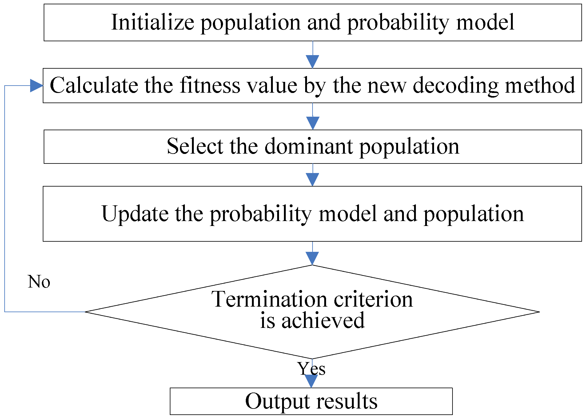
As for the process of EDA, the initialized population is randomly generated first, and the dominant individuals are selected according to their fitness. Then, the probability model is constructed from the dominant individuals to generate new ones. After the new population is generated, the termination criterion works to determine whether to stop this algorithm or not. This process is depicted in Figure 2.

4.1. Encoding, Decoding, and Dominant Individuals

The frequently utilized encoding method for solving FFSP is the arrangement-based encoding approach, in which only job sequence in the first stage is encoded and the jobs in the next stages are sorted according to dispatching rules like FCFS and SPT. Suppose that there are four jobs with an examplified code of [1 3 4 2], the first job is firstly processed and the third job is processed secondly. This encoding approach is simple to understand and complement, and thus is applied in this paper.

In regard to the population initialization, we adopt the random initialization method to ensure the population diversity. The computational complexity of this initialization method is $O(P_{size}n)$, where P_size is the population size and n the number of jobs.

On the ground of job sequence of the first stage, machine allocation, spindle speed, and job sequence at other stages are determined by decoding. In order to generate a feasible scheduling scheme, a dispatching rule is embedded in decoding to specify the job with the earliest completion time to be first processed, and any individual in the population can be decoded with Steps 1–3.

• Step 1: Choose an individual from the population, obtain its job sequence in the first stage, and set t = 1, $TE{C}^{*}=0$, $T_{{\mathsf{\pi }}_1,1}^c=0$ and $T_{{\mathsf{\pi }}_t,k}^m=0$.
• Step 2: Determine the processing machine and the spindle speed of all the jobs in current stage.

  • Step 2.1: Calculate the processing time ($T_{{\mathsf{\pi }}_{t}kl}^z$) and energy consumption ($E_{{\mathsf{\pi }}_t,k,l}$) of the current job (${\mathsf{\pi }}_t$) at all alternative speed levels on all available machines by Equations (2) and (11), respectively.
  • Step 2.2: Calculate the completion time ($T_{{\mathsf{\pi }}_t,k,l}^o$) of the job at all alternative speed levels on all available machines by Equation (26). Set $C{\max }_{{\mathsf{\pi }}_t,k,l}=T_{{\mathsf{\pi }}_t,k,l}^o$ and $TE{C}_{{\mathsf{\pi }}_t,k,l}=TE{C}^{*}+E_{{\mathsf{\pi }}_t,k,l}$.

    $$T_{{\mathsf{\pi }}_t,k,l}^o=\{\begin{array}{l}\max \{T_{{\mathsf{\pi }}_{t,}j-1}^c+T_{k^{\$}k}^d,T_{{\mathsf{\pi }}_{t-1},k}^m\}+T_{{\mathsf{\pi }}_{t}kl}^z,\forall t>1,j>1,k\in K_j,l\in N_{\mathsf{\pi }t,k}\\ \max \{T_{{\mathsf{\pi }}_t,j-1}^c+T_{k^{\$}k}^d,0\}+T_{{\mathsf{\pi }}_{t}kl}^z,\forall t=1,j>1,k\in K_j,l\in N_{\mathsf{\pi }t,k}\\ \max \{0,T_{{\mathsf{\pi }}_{t-1}k}^m\}+T_{{\mathsf{\pi }}_{t}kl}^z,\forall t>1,j=1,k\in K_j,l\in N_{\mathsf{\pi }t,k}\end{array}$$

    (26)
  • Step 2.3: Calculate the weighted target value using Equation (12), select the machine and the speed level with the smallest weighted target value for the job, and mark the index of the machine and corresponding speed level with $k^{*}$ and $l^{*}$.
  • Step 2.4: Set $T_{{\mathsf{\pi }}_t,k*}^m=T_{{\mathsf{\pi }}_t,j}^c=T_{{\mathsf{\pi }}_t,k*,l*}^o$, $TE{C}^{*}=TE{C}^{*}+E_{{\mathsf{\pi }}_t,k*,l*}$. If $t=n$, go to Step 3. Otherwise, set t = t + 1 and return to Step 2.1.
• Step 3: If $j=S$, the decoding process terminates. Otherwise, determine the job sequence in ascending order of the completion times, set j = j + 1, t = 1, $T_{{\mathsf{\pi }}_t,k}^m=0$, and return to Step 2. Calculate the final weighted target values of this individual using Equation (12).

Next, several dominant individuals are to be selected from the population so that the probability model can be applied. Based on the weighted target values, we sort all individuals in the ascending order of the target values, and then select the top $\mathsf{\eta }$% of individuals.

4.2. Population Updating Based on Probability Model

For the convergence, EDA applies an indicator function to extract the sequence characteristics of dominant individuals, and then constructs a probability model to guide the further population updating. Utilizing indicator functions, the position of a job in a dominant individual is signified and then the probability of this job arranged at all positions is statistically calculated. If the probability is higher, there is more chance for this job to stay at its previous position, and thus the population is updated gradually according to the mechanism of the roulette. The detailed steps of population updating based on probability model are as follows.

• Step 1: Set the indicator function $(I{S}_{ti}^l(0))$to zero, and set all elements in the probability matrix $({\mathrm{Pr}}_{ti}(0))$ to $1/n$.
• Step 2: At the gth generation, if job $i$ is on position $t$ of dominant individual $l$, set $(I{S}_{ti}^l(g))$ to 1. Repeat this process till all dominant individuals, all jobs and all positions have been iterated. Calculate the total value of job $i$ on position $t$ and then yield the probability $({\mathrm{Pr}}_{ti}(g+1))$ by using Equation (27).

  $${\mathrm{Pr}}_{ti}(g+1)=(1-a^s)\times {\mathrm{Pr}}_{ti}(g)+a^s\times {\displaystyle \sum _{l\in Sp}I{S}_{ti}^l(g)}/|Sp|,\forall g<G,t,i$$

  (27)
• Step 3: Update the population according to ${\mathrm{Pr}}_{ti}(g+1)$ by the roulette approach. Terminate the algorithm if termination criterion is met; otherwise, set g = g + 1 and return to Step 2.

5. Verification and Discussion

Computational experiments are conducted to verify the validity of the proposed mathematical model, and the effectiveness of the proposed EDA algorithm. All the experiments are performed on the computer with an Intel Core i5 processor running at 2.8 GHz and a main memory of 4G Bytes. The employed operating system is Windows 7 Professional. Note that the proposed mathematical model is programmed in GAMS/Dicopt and the proposed EDA is encoded in the programming language of MATLAB R2010a (The MathWorks, Inc., Natick, MA, USA).

To compare the performance of the proposed mathematical model and EDA, two smaller size turning cases are designed. Thus, there are three types of problems: a small-scale problem with four rolls, a medium-scale problem with 12 rolls, and a large scale problem with 60 rolls.

Before experiment, the weight of energy consumption was set to 0.8, which derived from Analytic Hierarchy Process (AHP) on the spot. Meanwhile, normalizing parameters of Cmax₀ and TEC₀ were determined for the three size experiments utilizing the heuristic rule in Section 3.2. Their values under small-scale, medium-scale, and large-scale circumstances were (3420 s, 29.07 MJ), (18,652 s, 289.17 MJ), and (26,763 s, 1294.1 MJ) respectively.

5.1. Parameter Calibration of EDA

EDA has three main parameters, namely population size noted as P_size, the ratio of dominant population noted as $\mathsf{\eta }\%$ which is equal to $\left|Sp\right|/\left|P_{size}\right|$, and learning rate noted as a^s. In this research, each factor has three levels: Psize (30, 50, 80), $\mathsf{\eta }$% (10%, 20%, 30%), and a^s (10%, 20%, 30%). We adopt an orthogonal experiment whose size is L9 (3³) to calibrate these parameters, and the stopping criterion is the elapsed time of 80 s. The numerical results are obtained through the heurisitc rule. Then TEC₀ and Cmax₀ are used as parameters to calculate weighted goals according to Equation (12), where $a=0.8$. Finally, the AOV of each experiment is obtained as shown in

Table 1. Orthogonal experiment of EDA.

Combination	Level			AOV
	Psize	η%	as
1	80	30	0.1	0.9239
2	30	20	0.3	0.9237
3	80	10	0.3	0.9229
4	30	30	0.2	0.9243
5	50	30	0.3	0.9239
6	80	20	0.2	0.9239
7	50	20	0.1	0.9233
8	50	10	0.2	0.9230
9	30	10	0.1	0.9232

, where AOV is the average value of the weighted targets for 30 tests.

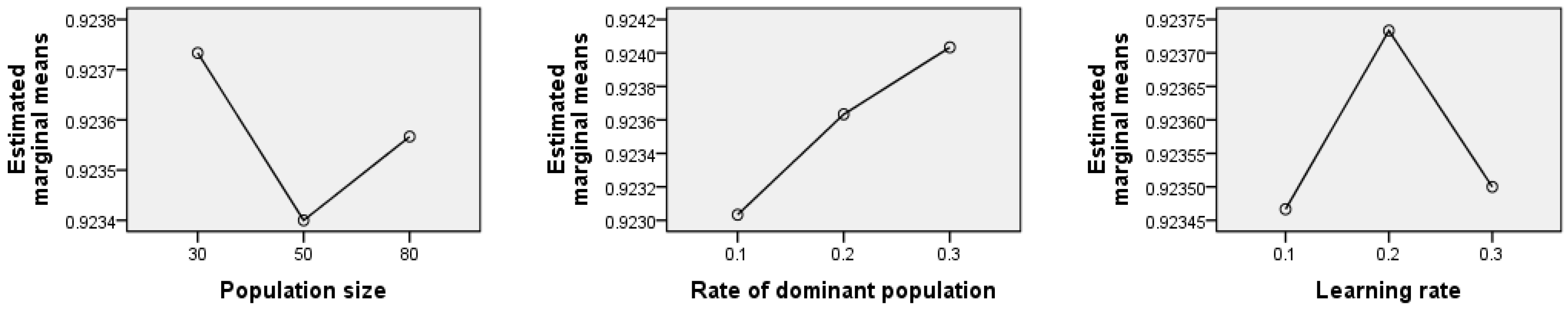
Table 1 shows under the third combination of (0, 10%, 0.3), the AOV value is the smallest, and thus the third combination is the best. However, when these parameters are invetsigated independently in Figure 3, we note that the best population size is 50, the best rate of dominant population 10% and the best learning rate 10% or 30%. The above results are not in accordance with that in the third combination. Considering the incompleteness of the orthogonal experiment, two more tests of the combinations of (50, 10%, 0.1) and (50, 10%, 0.3) are performed, and their AOVs are 0.9229 and 0.9228. Taking these 11 experiments into account, we draw the conclusion that the optimal parameter combination is (50, 10%, 0.3) for the population size, rate of dominant population, and the learning rate.

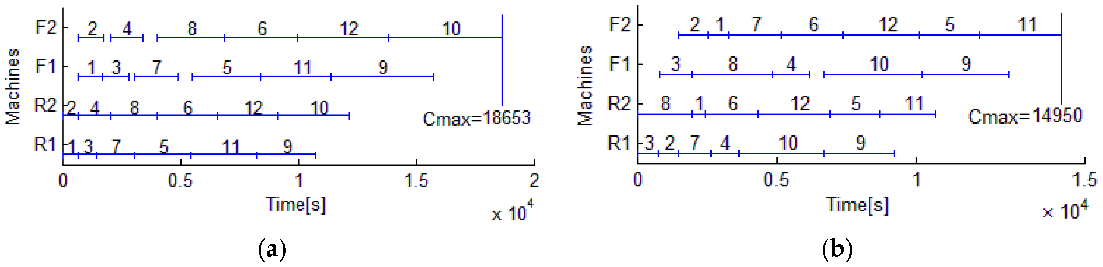
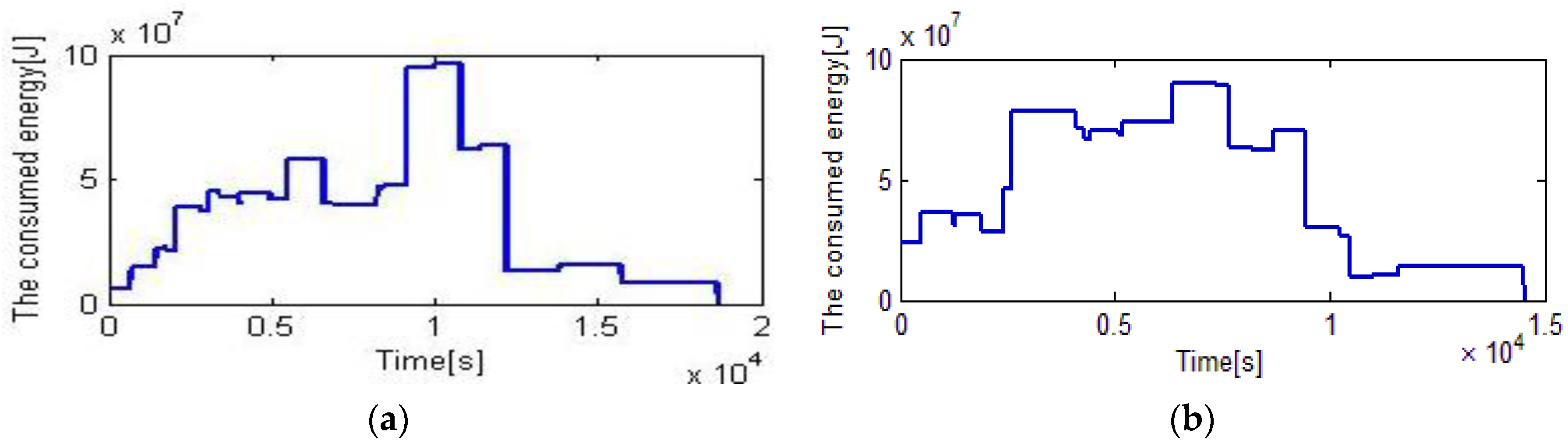
The EDA is applied to schedule 12 rolls, and the termination criterion is that the elapsed time reached 80 s. These jobs are completed in 14,594 s, and 4058 s is saved compared with 18,652 s which is the makespan of the original scheduling by the heuristic rule. The total energy is 280.08 MJ, and 9.09 MJ is saved compared with the original scheduling. The results of the heuristic rule are depicted in Figure 4a, Figure 5a and Figure 6a, and the results of EDA are shown in Figure 4b, Figure 5b, and Figure 6b.

5.2. Experimental Results of the Motivating Example

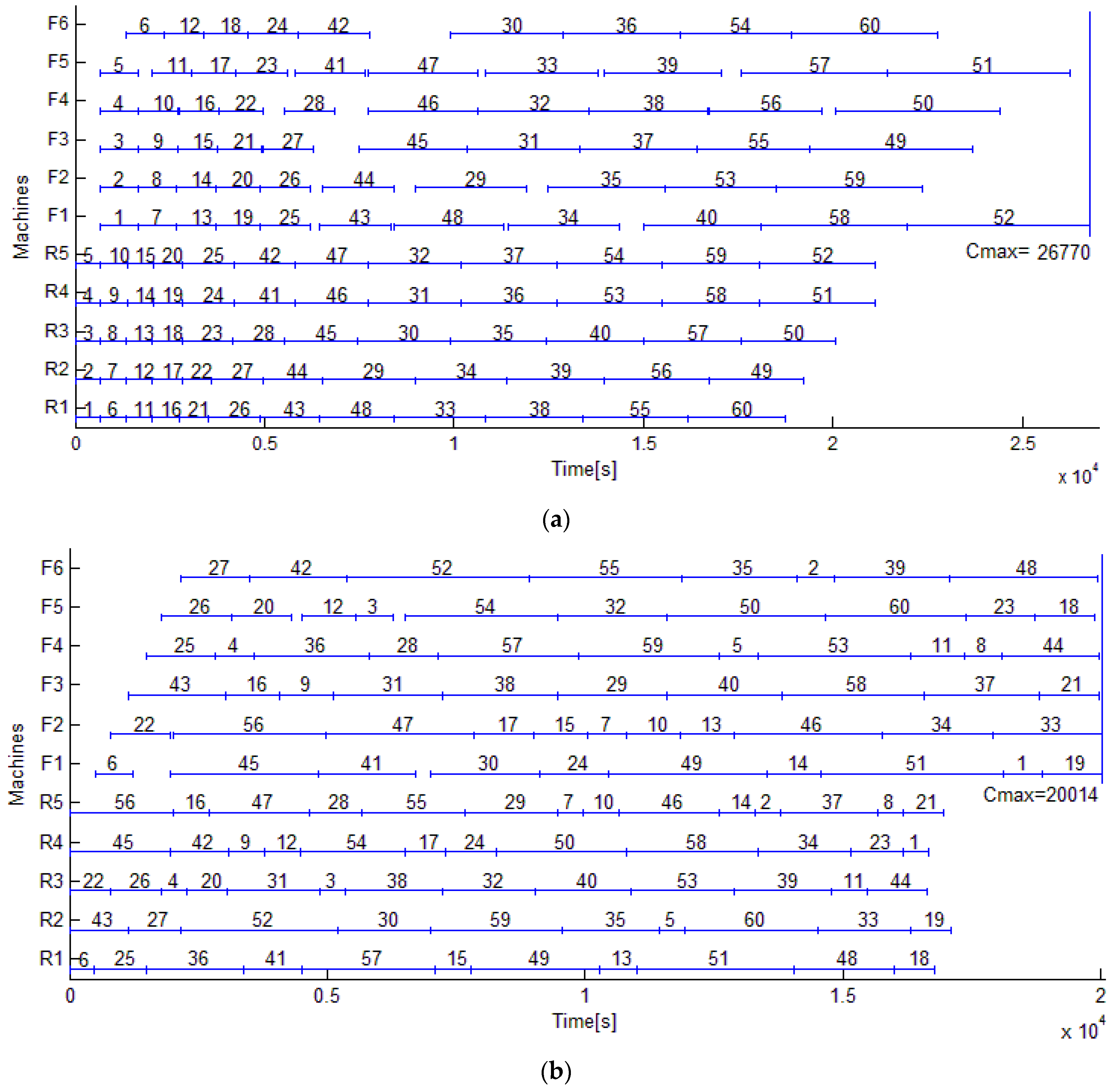
Figure 7a,b compare the Gantt charts of 60 rolls by heuristic rule and by EDA. Apparently, the derived maximum completion time by EDA is shortened by 6749 s or by 25.22% compared with that by heuristic rule. Only tiny idle times remain in the Gantt chart by EDA.

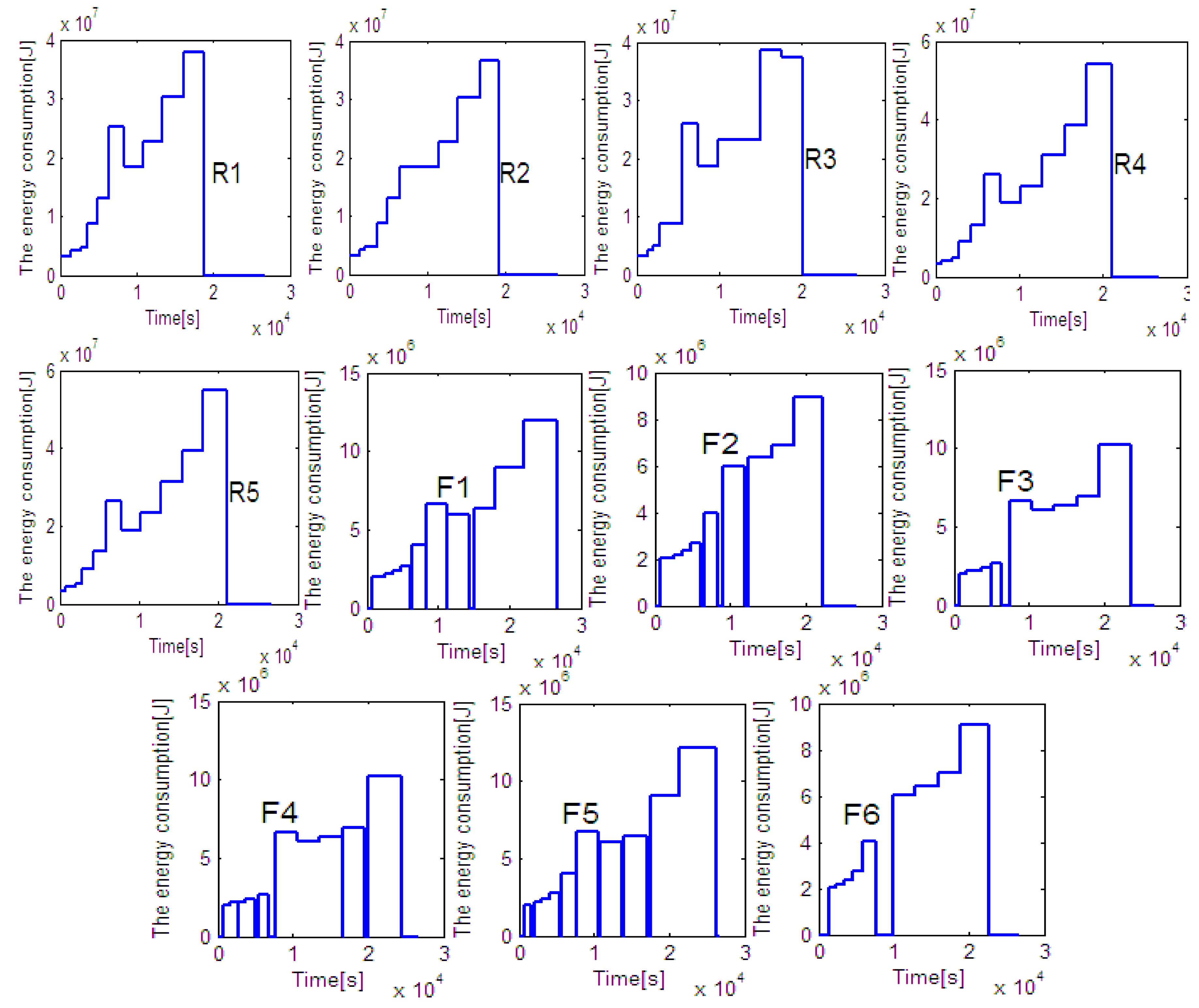
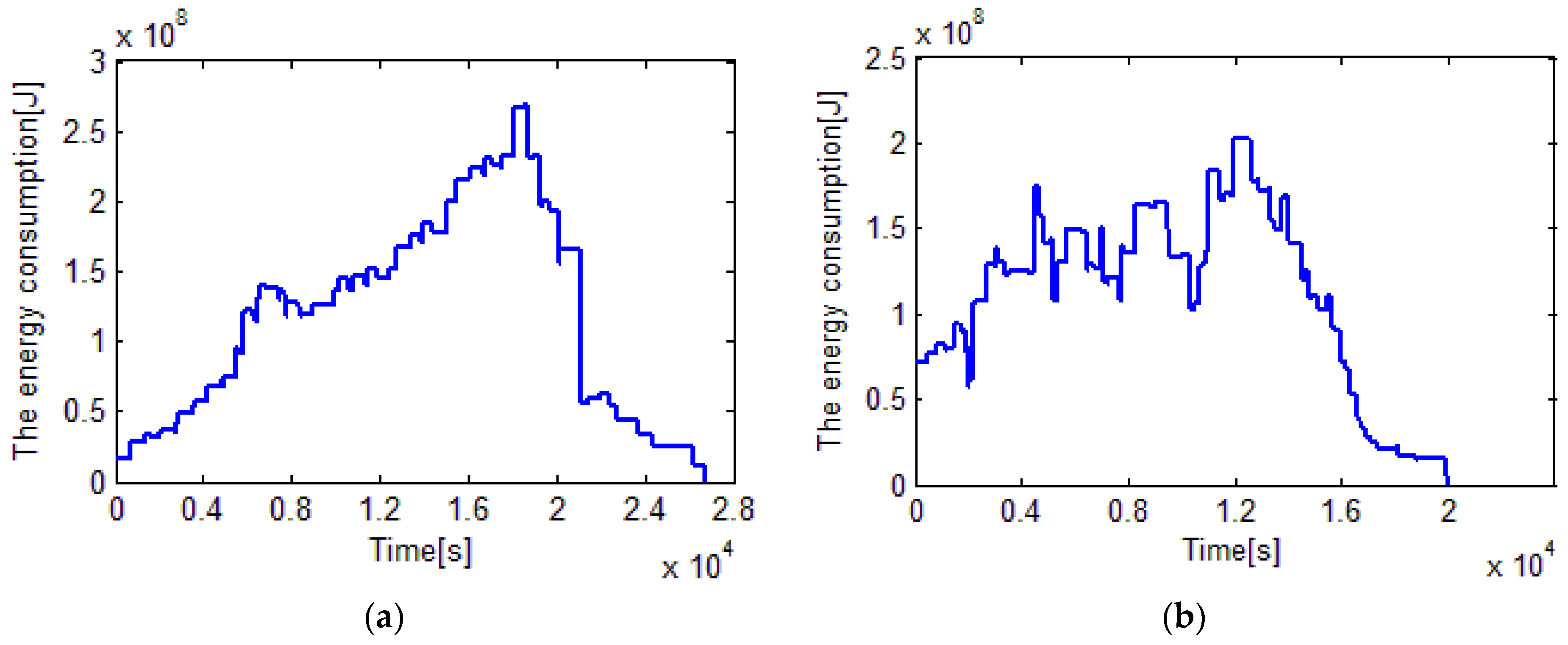
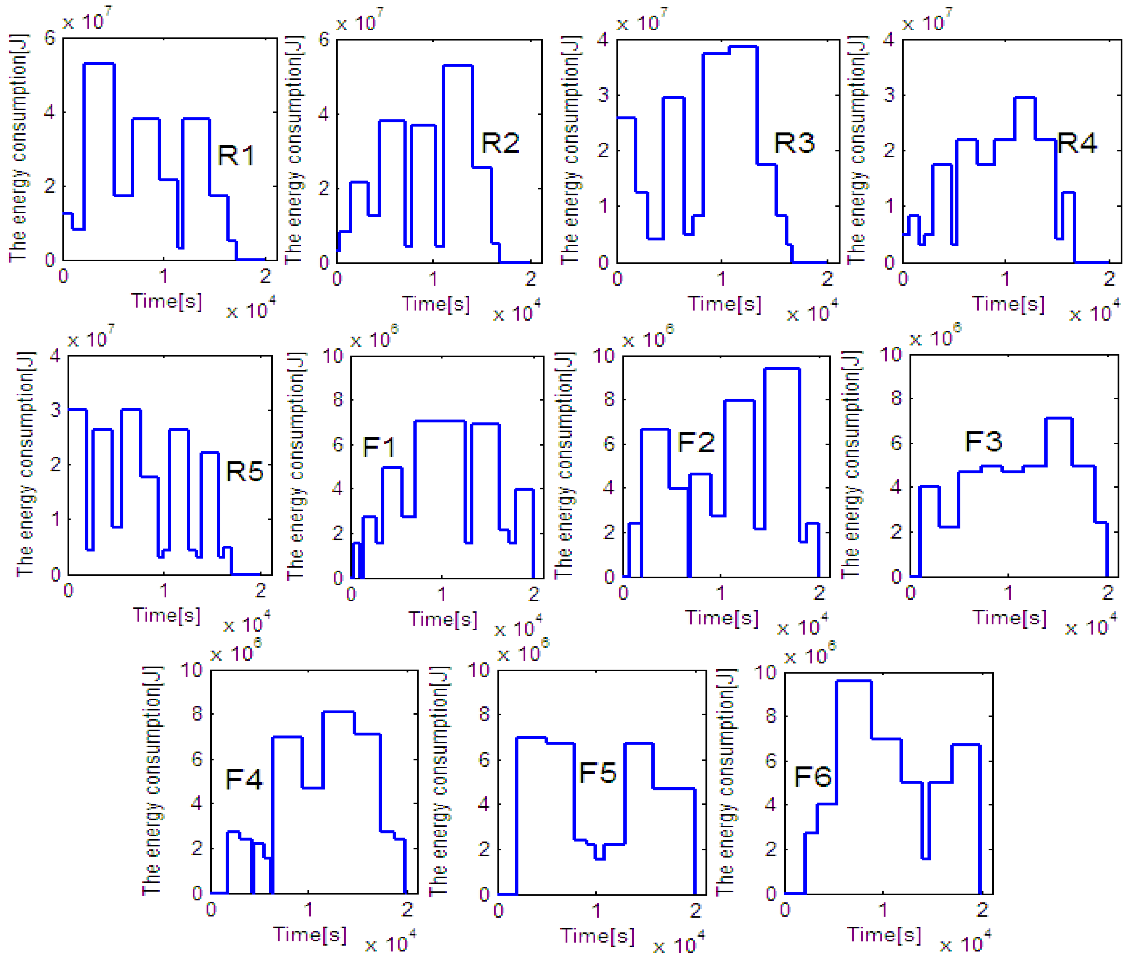
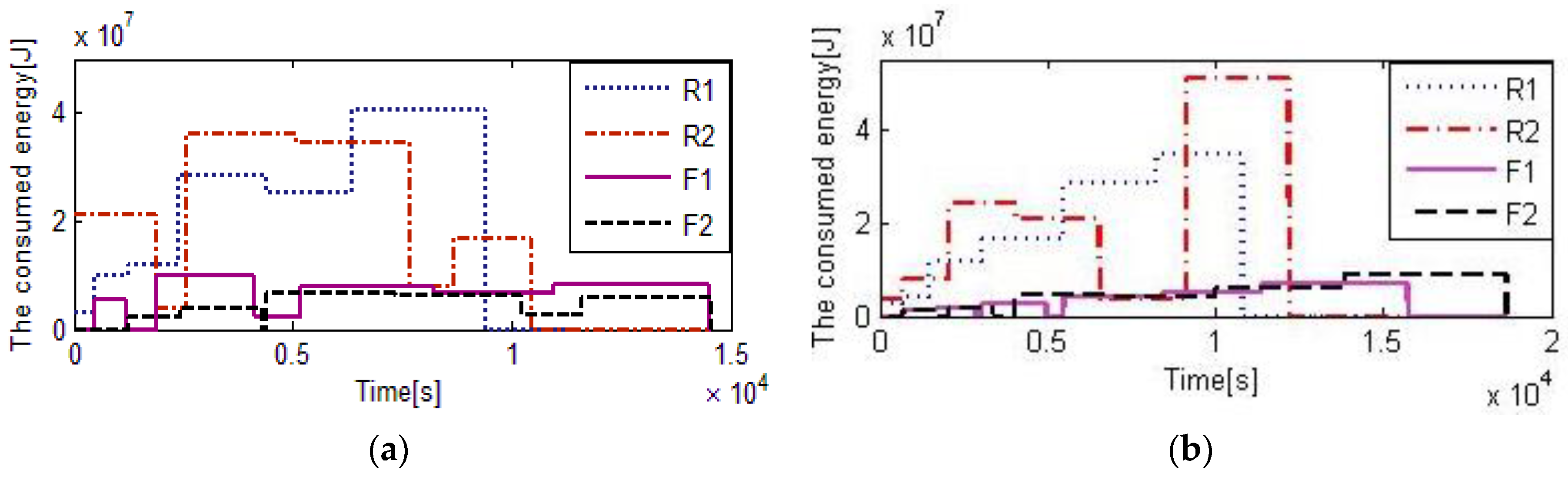
With respect to the consumed energy, Figure 8b shows that the peak value of energy comsumption of 60 rolls by EDA is less than 250 MJ, while that by heuristic rule is nearly 300 MJ. The total energy consumed by the proposed EDA and the heuristic rule is 1223.2 MJ and 1294.1 MJ. In other words, 70.9 MJ or 5.48% of the total energy is saved by the proposed EDA. Note that, the energy consumptions of all lathes are reported in Figure A1 and Figure A2 in Appendix.

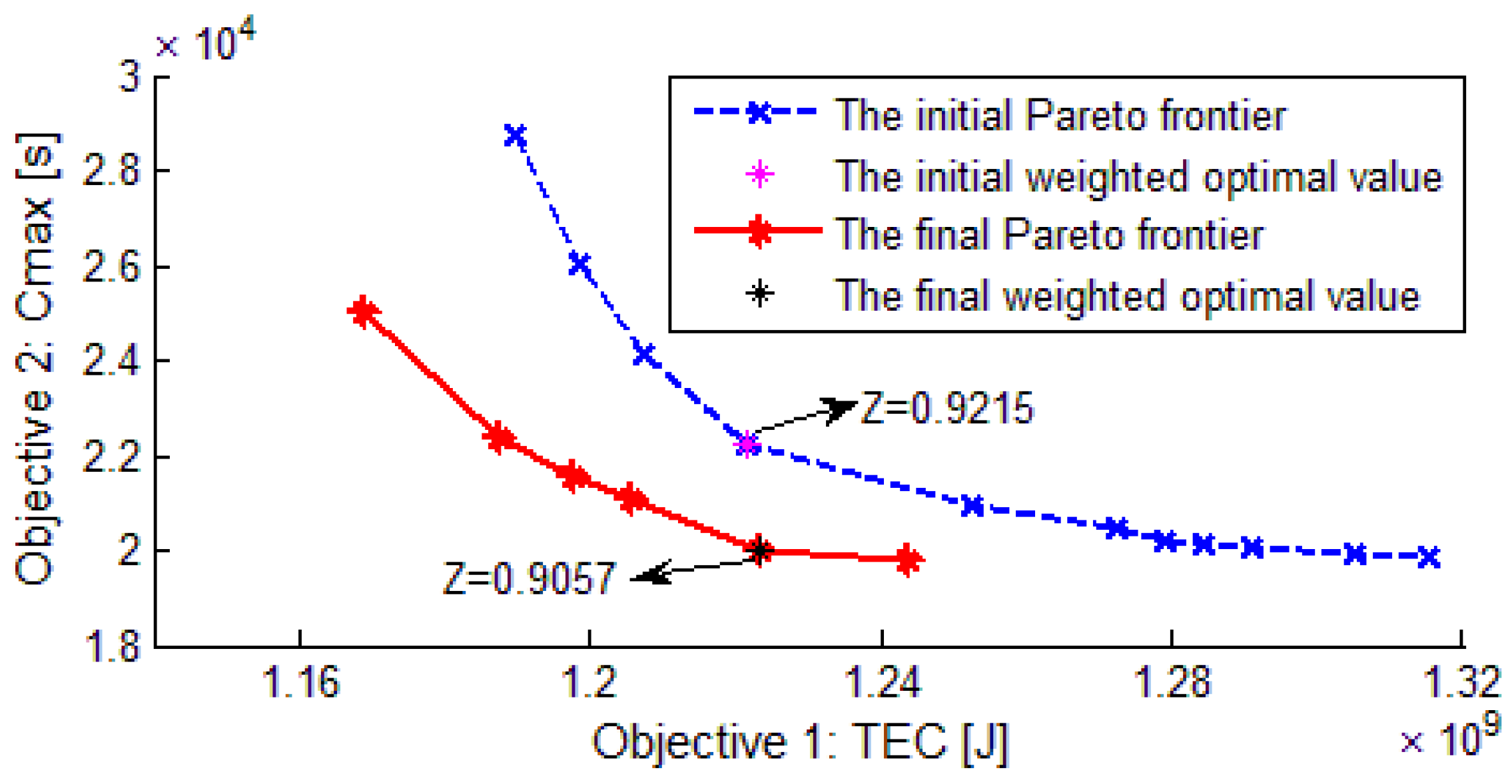
Figure 9 reports the Pareto frontier of the population. We can see the siginificant improvement of the Pareto frontier from the first to the final generation, which clearly demonstrates a bidirectional and synchronous optimization of the two objectives. Obviously, the optimal solution of the proposed mathematical model, in which both the total energy consumption and makespan are weighted, lies on the curve of Pareto frontier.

Table 2. Comparison of results.

Solving Methods	Small Scale				Medium Scale				Large Scale
	Cmax (h)	TEC (MJ)	Z (%)	Time (s)	Cmax (h)	TEC (MJ)	Z (%)	Time (s)	Cmax (h)	TEC (MJ)	Z (%)	Time (s)
MINLP	0.91	23.40	83.54	0.66	4.22	275.33	92.47	4.2 × 103	out of memory			>7.2 × 104
EDA	0.92	23.40	83.71	10.00	4.05	280.08	93.13	80.00	5.56	1223.2	90.57	180.00

compares the results obtained by the proposed EDA and that solved by GAMS/Dicopt solver for the MINLP model. It shows that, for small-scale problems, Dicopt solver outperforms the proposed EDA in both objectives during the acceptable time. For medium scale cases, the Dicopt solver takes much more time than the proposed EDA, but it produces a tiny improvement in the weighted target. For large-scale cases, the proposed EDA is absolutely superior over the Dicopt solver which cannot provide a feasible solution for the limited memory of the computer.

In summary, using the proposed EDA, energy-efficient scheduling can be achieved effectively. Moreover, makespan and the total energy consumption can be reduced simultaneously, and hence production efficiency improvement and energy saving are realized.

5.3. Discussion

The weight used in this paper is determined by AHP after investigating the preferences of managers in the real case. In order to clarify the weight range, sensitivity analysis experiments are conducted. Experiments show that when the weight is 1, the makespan is 13.41 h and the TEC is 1218.2. Although this TEC is slightly better than that under other circumstances, the makespan is particularly worse. Actually, this result originates from the single-objective optimization of the total energy consumption and the ignorance of makespan under this circumstance. Therefore, the weight value of 1 is excluded from the weight range and then the weight range is limited by (0, 0.8).

Table 3. Two objectives under different weights.

Weights	TEC (MJ)	Cmax (h)
0.8	1223.2	5.56
0.6	1228.5	5.54
0.5	1234.0	5.50
0.4	1240.6	5.45
0.2	1243.1	5.43
0	1248.5	5.41
Relative difference	2.03%	2.76%

shows the results after this adjustment. It demonstrates that the relative difference of total energy consumption is 2.03%, and that of makespan is 2.76%. Therefore, a conclusion can be reached that the two objectives are not sensitive to the weight when it ranges from 0 to 0.8.

Besides, in order to find out the underlying reasons, three different optimization goals and two optimization methods are analyzed and compared. Three optimization goals are given: (1) the comprehensive goal by weighting the consumed energy and completion time (Obj_C); (2) the single target only considering the consumed energy (Obj_e); and (3) the single target only considering makespan (Obj_t). The two different optimization methods are given as follows: (1) optimizing the scheduling scheme and spindle speed synchronously (Opt_S); and (2) optimizing the scheduling scheme after determining the appropriate spindle speed (Opt_o). The following experiments contain six combinations of the above optimization goals and methods. For testing the robustness of the proposed EDA, it is run 30 times for each combination. The stopping criterion is fixed to a given maximum elapsed CPU time of 180 s. To evaluate the different optimization goals and methods, firstly Cmax, TCE, and the weighted objective of the best scheduling for each experiment are recorded; secondly the objectives are respectively analyzed by the repeated measures in IBM SPSS 19, in which optimization goals are set as within-subject effects and optimization methods as between-subject effects. The results are shown in

Table 4. Descriptive statistics.

Opt Goals	Opt Schemes	Weighted Objectives		Cmax		TEC
		Mean (%)	Std. Deviation	Mean (s)	Std. Deviation	Mean (KJ)	Std. Deviation
Obj_C	Opt_S	0.9182	0.0009	20,138.03	114.48	1,088,720.23	595.05
	Opt_o	0.9766	0.0009	24,327.10	115.38	1,127,157.80	808.95
	Total	0.9474	0.0293	22,232.57	2115.28	1,107,939.02	19,393.75
Obj_e	Opt_S	1.5976	0.0043	112,651.53	570.03	1,071,912.00	0.00
	Opt_o	1.7903	0.0036	134,722.73	475.01	1,111,200.00	0.00
	Total	1.6940	0.0972	123,687.13	11,140.88	1,091,556.00	19,809.78
Obj_t	Opt_S	0.9212	0.0015	20,388.53	172.42	1,090,310.33	617.99
	Opt_o	0.9794	0.0020	24,503.33	236.15	1,129,263.87	1082.78
	Total	0.9503	0.0294	22,445.93	2084.87	1,109,787.10	19,660.57

,

Table 5. Multivariate tests of weighted objectives.

Effect		Value	F	Hypothesis df	Error df	Sig.	Partial Eta Squared
Objs	Pillai’s Trace	1.000	1,050,284.622	2.000	57.000	0.000	1.000
	Wilks’ Lambda	0.000	1,050,284.622	2.000	57.000	0.000	1.000
	Hotelling’s Trace	36,852.092	1,050,284.622	2.000	57.000	0.000	1.000
	Roy’s Largest Root	36,852.092	1,050,284.622	2.000	57.000	0.000	1.000
Objs * methods	Pillai’s Trace	0.997	8518.901	2.000	57.000	0.000	0.997
	Wilks’ Lambda	0.003	8518.901	2.000	57.000	0.000	0.997
	Hotelling’s Trace	298.909	8518.901	2.000	57.000	0.000	0.997
	Roy’s Largest Root	298.909	8518.901	2.000	57.000	0.000	0.997

Note: (Objs * methods) means the interactions between optimization goals and optimization methods.

and

Table 6. Between-subjects effects on weighted objectives.

Source	Type III Sum of Squares	df	Mean Square	F	Sig.	Partial Eta Squared
Intercept	257.993	1	257.993	36,964,741.896	0.000	1.000
Methods	0.478	1	0.478	68,527.167	0.000	0.999
Error	0.000	58	6.979 × 10−6

.

From Table 4, we note that in the columns of weighted objective and Cmax, Obj_C yield the means of 0.9474 and 22,232.57 which are both better than that of Obj_e and Obj_t. In TEC, the mean of 1,107,939.02 obtained by Obj_C is lower than that of Obj_t. Therefore, adopting the weighted goal to measure energy-efficient scheduling is suitable for optimizing the comprehensive objective and makespan. In TEC, the means of 1,091,556.00 is the lowest; however, the Obj_e is not often used in real production due to the long makespan, which is 123,687.13 s, more than four times longer than that of Obj_C and Obj_t. The reason is that all the jobs are assigned on the most efficient machine while the other machines are idle. Therefore, among the three optimization goals, the weighted objective is the best measure method for energy-efficient scheduling. Table 4 also shows that Opt_S yields lower means than Opt_o, no matter which of the three optimization goals is adopted. Therefore, optimizing the scheduling scheme and spindle speed synchronously not only saves the consumed energy but also shortens the makespan. Optimizing the scheduling scheme and turning parameters synchronously has a great effect on environment protection and production efficiency.

Table 5 also shows the multivariate tests of weighted objectives. Since all the differences are significant (0.000 < 0.05), the optimization goals can affect the weighted objective significantly. The interactions between optimization goals and optimization methods also affect the weighted objective significantly. The differences of multivariate tests of Cmax and TEC are also significant, so the optimization goals and the interactions can affect Cmax and TEC, too. The data of the multivariate tests of Cmax and TEC are not reported here since they are similar to Table 5.

Table 6 shows the tests of between-subjects effects on weighted objectives. Since the difference is significant (0.000 < 0.05), the optimization method can affect the weighted objective significantly. The differences of between-subjects effects on Cmax and TEC are significant, so the optimization methods can also affect Cmax and TEC significantly.

All in all, we find that different optimization goals and methods affect the Cmax and TEC significantly, so both environmental and production benefits can be enhanced simultaneously by optimizing the spindle speed and scheduling scheme, which is the first realization in this regard.

6. Conclusions

Reducing the energy consumption is increasingly believed to be an effective environment protection measure in manufacturing industry. The optimization of the energy-efficiency scheduling in flexible flow shops with parallel machines can contribute to energy consumption redution and production efficiency improvement synchronously. In this paper, the following achievements have been obtained towards the energy-efficient scheduling in turning shops:

(1)

A mixed integer nonlinear programming model is established by optimizing the spindle speed and scheduling scheme simultaneously, and subsequently, small-scale and medium-scale problems are solved by the GAMS/Dicopt;

(2)

For large-scale problems, an effective EDA algorithm is proposed in which a dispatching rule is embedded in decoding to specify the job with the earliest completion time to be first processed, and the population is updated utilizing the probability of the dominant individuals;

(3)

The experiment results show that: (1) the proposed algorithm can reduce the energy consumption to a certain extent and shorten the makespan to a large degree; and (2) there is a positive correlation between the energy consumption and makespan.

In future research, other turning parameters such as cutting depth and feed rate will also be taken into consideration so as to further improve the energy efficiency. More types of production shops, such as no-wait or no-idle flow shops, as well as other constraints such as due date will be studied.