Study on Retrieval of Chlorophyll-a Concentration Based on Landsat OLI Imagery in the Haihe River, China

Abstract

The optical complexity of urban waters makes the remote retrieval of chlorophyll-a (Chl-a) concentration a challenging task. In this study, Chl-a concentration was retrieved using reflectance data of Landsat OLI images. Chl-a concentration in the Haihe River of China was obtained using mathematical regression analysis (MRA) and an artificial neural network (ANN). A regression model was built based on an analysis of the spectral reflectance and water quality sampling data. Remote sensing inversion results of Chl-a concentration were obtained and analyzed based on a verification of the algorithm and application of the models to the images. The analysis results revealed that the two models satisfactorily reproduced the temporal variation based on the input variables. In particular, the ANN model showed better performance than the MRA model, which was reflected in its higher accuracy in the validation. This study demonstrated that Landsat Operational Land Imager (OLI) images are suitable for remote sensing monitoring of water quality and that they can produce high-accuracy inversion results.

1. Introduction

Chlorophyll-a (Chl-a) concentration can be used as a direct indicator of the ecological state of a water body. For example, an algal bloom can degrade water quality in rivers, lakes, and reservoirs, and Chl-a concentration has been shown useful as an indicator for measuring the abundance and variety of phytoplankton and/or the algal biomass [1]. Since the 1990s, the development of satellite technology, greater understanding of the spectral signature of water quality parameters, and the development of mathematical models have led to semi-empirical methods becoming the principal means with which to monitor water quality remotely. Studies on water environmental protection and the monitoring of water quality have become increasingly important because of the severe environmental problems affecting surface water [2]. Point-to-surface and static-to-dynamic monitoring of water quality are required urgently; however, it is difficult to perform long-term monitoring over large areas. Research based on remote sensing techniques and the spectral characteristics of water is extremely valuable for large-scale monitoring of water quality, especially when traditional water sampling analysis methods are restricted by factors such as labor and material costs, and climatological and hydrological conditions. Inversion of water quality parameters using remote sensing technology can improve the monitoring of surface water quality and derive dynamic water quality information in real-time. Thus, this technique represents an important complement to regular water quality monitoring, and it can provide a robust scientific basis for governmental decision-making in relation to the ecological economic zone.

Chl-a concentration has been used as an important index to reflect water quality conditions [3,4]. Accurate information on the spatiotemporal variation of Chl-a concentration can contribute to improved understanding of water quality status and assist water-resource management. Traditional methods used to monitor Chl-a concentration, e.g., spectrophotometry, have many limitations: high cost, complex method of operation, restriction of observations to specific regions and/or specific times, and long monitoring periods. The lack of in situ real-time monitoring data on the quality and optical properties of inland water bodies renders it difficult to determine the spatiotemporal variation of Chl-a concentration. Satellite remote sensing technology has shown great potential in providing spatial distribution patterns of Chl-a [5]. The application of such technology can be cost effective, shorten the period of observation, and increase the temporal frequency of sampling. Furthermore, in conjunction with an accurate and efficient inversion model, the technology can realize real-time, synchronous, large-area, and continuous monitoring of Chl-a concentration in a target area [6]. Thus, remote sensing techniques are able to overcome the shortcomings of traditional observational methods. In particular, improvements of the geometry and the spectral resolution associated with remote sensing technology have presented new possibilities for the evaluation of water resources via the monitoring of Chl-a concentration.

Substances that affect the light intensity and the spectral distribution in surface water can be divided into three categories: pigment of plankton algae, suspended matter and yellow substances. The pigment of plankton algae and suspended matter are usually characterized by Chl-a and total suspended matter, and these two parameters are usually used as indices of inversion. The concentrations of Chl-a and suspended matter have obvious similarities in terms of scope of spatial autocorrelation and they have similar spatial distribution patterns [7]. The optical properties of water are relatively complex, and they vary between different waters, making it difficult to build a widely applicable and high-precision inversion model of water quality parameters [8].

Numerous studies have been conducted on water quality in various water bodies using a variety of satellite platforms and data, e.g., Thematic Mapper (TM) data [9,10], Systeme Probatoire d’Observation de la Terre-High Resolution Visible (SPOT-HRV), National Oceanic and Atmospheric Administration/The Advanced Very High Resolution Radiometer (NOAA/AVHRR), Airborne Visible Infrared Imaging Spectrometer (AVIRIS) [11], Compact Airborne Spectrographic Imager (CASI) [12], Analytical Spectral Devices (ASD) spectral data [13], Indian Remote Sensing (IRS)-1C image data [14], China–Brazil Earth Resources Satellite (CBERS)-2 Change Coupled Device (CCD) image data [15], Airborne Imaging Spectrometer for Applications (AISA) imaging spectrum data [16], Moderate Resolution Imaging Spectroradiometer (MODIS) [17], MEdium Resolution Imaging Spectrometer (MERIS) [18,19], and Hyperion [20,21]. The most practical and widely used remote sensing data are TM data. However, hyperspectral data obtained from AVIRIS, CASI and ASD can provide detailed information in bands relevant to water. NOAA/AVHRR and MERIS data are generally used to study ocean water and they have been shown to achieve good results. The most commonly used water inversion methods use conventional remote sensing imagery and hyperspectral data to establish an empirical algorithm that corresponds to an inversion model that calculates the required water quality parameters. Chl-a concentration retrieval algorithms can be divided into empirical algorithms [22,23], semi-analytical algorithms [24,25], and analytical algorithms [26,27,28]. A quantitative inversion of Chl-a concentration can be realized by logarithmic and arithmetic operations of digital number (DN) of different wavelengths retrieved by remote sensors, remote sensing reflectance, apparent reflectance, or water surface reflectance. The most commonly used statistical models include the ratio method, establishing a regression equation by combining different bands, and the fluorescence method. The improvement of the inversion accuracy of water quality parameters was the primary objective of the present research.

The Haihe River in China is Tianjin’s largest natural water resource and, therefore, the water quality of the Haihe River is very important. An efficient inversion model for the determination of Chl-a would allow the environmental department to monitor the water quality of the Haihe River quickly and dynamically, and to further strengthen the management of the river. This study used field and satellite-derived data of the Haihe River to develop an effective algorithm for the determination of Chl-a concentration. Accurate validation and sophisticated algorithm development are primary requirements for the reliable retrieval of remote sensing data. An artificial neural network (ANN) is a powerful method of pattern recognition that has been used in many fields including business, industry, engineering, and science, and it is a technique that has been applied to predict algal blooms [29]. This study built mathematical regression analysis (MRA) and ANN models for the Haihe River to inverse Chl-a concentration through precise prediction and evaluation of the relationship between input and output.

2. Study Area and Data Preprocessing

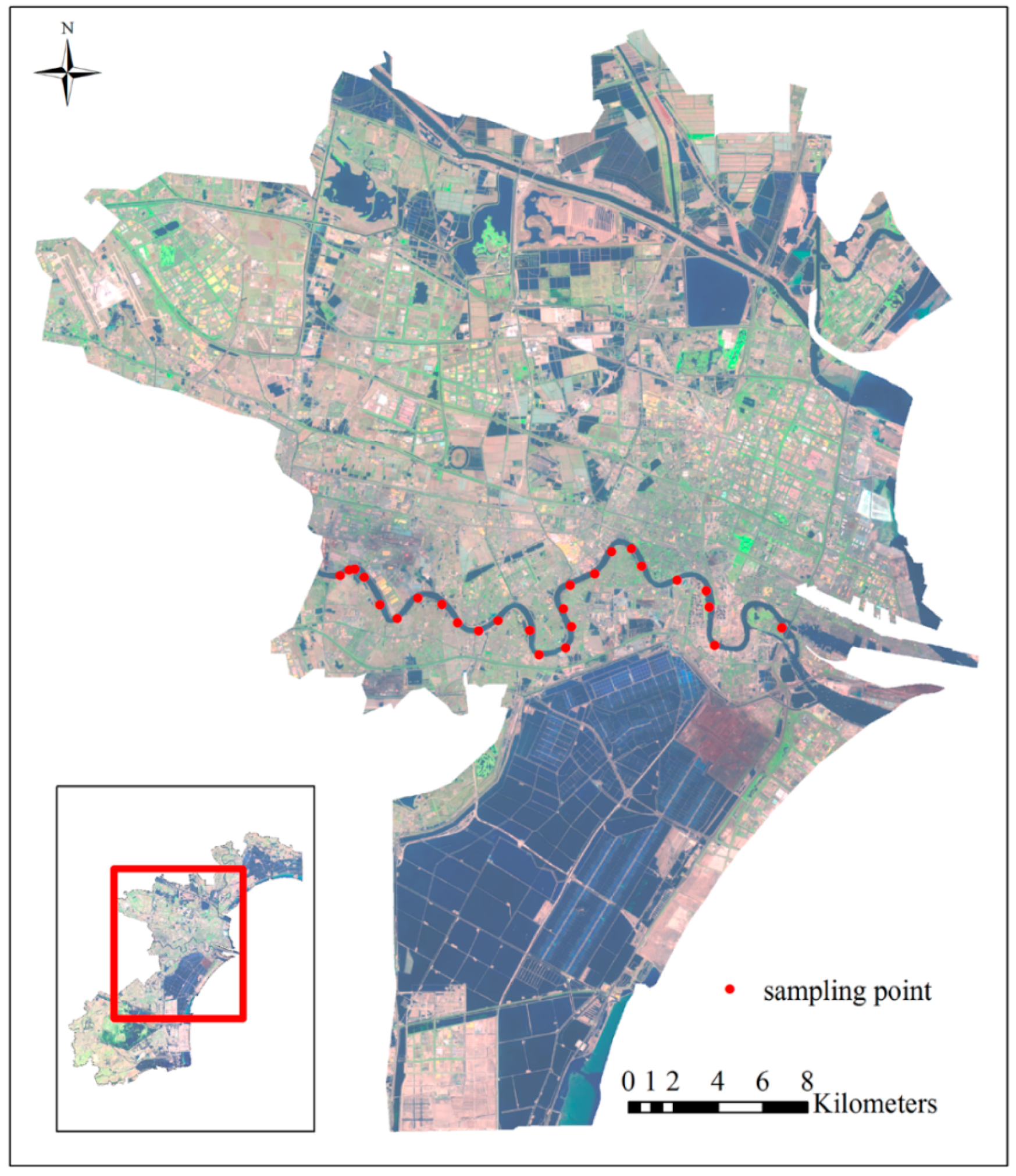
2.1. Study Area

The study area is the section of the Haihe River in the Binhai New Area located in the eastern part of Tianjin (38°40′–39°00′N, 117°20′–118°00′E) covering an area of 2270 km² (Figure 1). The Haihe River is the largest river in North China. Its length is 2458.4 km and it flows through Hebei Province, the cities of Beijing and Tianjin, and Shandong Province, Owing to its geographical location, the region is affected by both subhumid warm temperate continental monsoon and oceanic climates. The annual runoff discharge of the Haihe River is 22.8 billion cubic meters, more than half of which is accounted for by rainfall recharge. The sediment concentration of the river ranks second only to that of the Yellow River. Over the years, industrial drainage and urban sewerage have caused serious pollution of the Haihe River, thus, monitoring and management of the Haihe River water quality is necessary.

2.2. Remote Sensing Data Preprocessing

The remote sensing images used in the study were Landsat-8 acquired on 22 April 2014 in the red, green and blue wavelengths of bands 7, 5, and 4, respectively. First, the images were preprocessed through radiometric calibration, atmospheric correction, and geometric correction to obtain remote sensing reflectance of water pixels. Using ENVI 5.1 (Exelis Visual Information Solutions, Boulder, CO, USA, 2014), the Landsat-8 Operational Land Imager (OLI) Fast Line-of-sight Atmospheric Analysis of Spectral Hypercubes (FLAASH) processing tool was used for the atmospheric correction and the georeferencing tool was used for the geometric correction of the images. The correction method adopted a quadratic polynomial fit and the precision of the geometric correction was within 0.5 pixels. Once the area of interest was established, the geometrically corrected images were clipped and land information was removed, all of which facilitate analysis and reduce data-processing time. Based on the remote sensing image, a section of the Haihe River was selected as the study area. Specific points were then identified within the study area, from which water samples were physically collected. The selection principle was to achieve one sampling point per kilometer. When collecting the water samples in the field, the position of each water quality sampling point was recorded using a global positioning system (GPS) receiver and its latitude and longitude were transformed to the WGS_1984_UTM_ZONE_50N coordinate system. The locations of the water quality measuring points are shown in Figure 1.

2.3. Data Collection

The sample collection was performed along the Haihe River on 22 April 2014, and 26 water samples were collected and taken back to the laboratory. The water samples were divided into several parts, one of which was intended for the measurement of Chl-a concentration. Before undertaking the measurements of the spectral properties of the water samples, 30 samples storage containers were prepared, on each of which was marked the sampling point number. Some of the sampled water was used for cleaning the corresponding sample storage containers. Then, the containers were filled with sample water and stored in storage boxes at room temperature. The spectral information of the water at the sampling locations was collected using a portable spectrometer, and the coordinate positioning information including latitude and longitude was acquired using a GPS receiver. On 23 April 2014, the Chl-a concentration of each sample was measured using a spectrophotometric method. Water quality parameters were measured using a ET99732 multiparameter analyzer. In total, 26 observations were recorded.

2.4. Sample Processing and Measurement in Laboratory

The accurate determination of Chl-a concentration has great significance regarding the assessment and prediction of water eutrophication condition. The absorbance of the Chl-a in the water samples was measured at four wavelengths: 750, 663, 645, and 630 nm using a spectrophotometer, and the Chl-a concentration was calculated according to Equation (1) with consideration of the method of Chl-a extraction and water quality of the Haihe River. In recognition of the shelf life of the water samples, they were processed and analyzed in a laboratory the day after collection in the field. The specific steps of sample processing for the determination of Chl-a concentration were as follows:

(1)

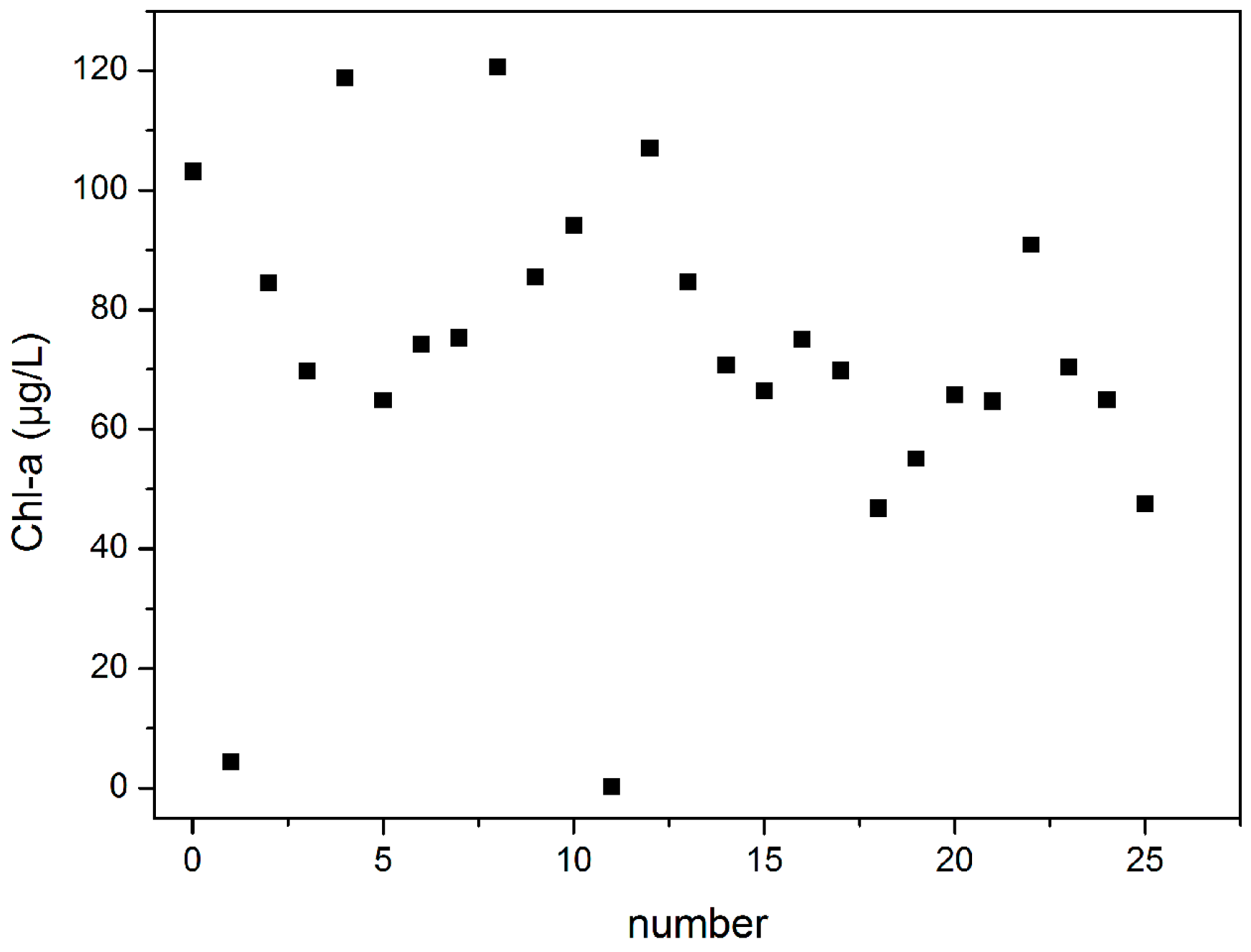
Water samples were collected from 26 points along the Haihe River in the Binhai New Area of Tianjin and placed into appropriately numbered empty bottles.

(2)

In the laboratory, the water samples were agitated and a 100 mL sample was extracted into a measuring cylinder, ensuring that the line of sight and the concave liquid surface were maintained at the same level throughout the process.

(3)

The prepared water samples were filtrated using cellulose ester microporous membrane filters (diameter: 47 mm; pore size: 0.45 μm) under the action of a vacuum.

(4)

After filtration, the membrane filter was removed and the sample placed into a one-time centrifugal pipe plug, to which 100 mL of ethanol was added with a pipette and the mixture was shaken.

(5)

Steps (2)–(4) were repeated for the remaining samples and then the samples were placed in a fridge for 48 h.

(6)

The solution and filter membrane were placed into a one-time centrifuge tube and centrifuged 3 min at 3000 rpm.

(7)

The colorimetric was cleaned with ionized water and the spectrophotometer corrected.

(8)

After centrifugation, the supernatant solution was placed into the colorimetric ware, and the wavelength absorbance values at 630, 645, 663, and 750 nm using the spectrophotometer and recorded. The value recorded at 750 nm was used for rectifying the turbidity of the extracted solution. When the absorbance value of the light path measured at 1 cm was >0.005, the sample was centrifuged again.

The Chl-a concentration was determined using the following formula [30]:

$${\mathsf{\rho }}_{\text{Chl-a}}=(11.64\times (D_{663}-D_{750})-2.16\times (D_{645}-D_{750})+0.10\times (D_{630}-D_{750}\left)\right)\times V_1/(V\times \delta )$$

(1)

where ρ_Chl-a denotes the Chl-a concentration of the water sample (units: μg/L); D₆₃₀, D₆₄₅, and D₆₆₃ denote the corrected absorbance values measured at the wavelengths of 630, 645, and 663 nm, respectively, subtracted from that measured at the wavelength of 750 nm (D₇₅₀ denotes the absorbance value measured at the wavelength of 750 nm); V denotes the volume of water sample (units: L); V₁ denotes the volume of the extract after constant volume (units: mL); and δ is the optical path length of the measurement cell (units: cm).

The Chl-a concentrations of the 26 samples, measured by the spectrophotometric method outlined above, are shown in Figure 2. The mean, minimum, maximum, and median Chl-a concentrations are 76.37, 0.21, 120.66, and 70.54 μg/L, respectively; the standard deviation (SD) is 21.43 μg/L, and the coefficient of variation (CV) is 28.06 μg/L.

3. Chl-a Concentration Inversion Methods

3.1. Chl-a Concentration Inversion Based on a MRA Model

Following the radiometric calibration and atmospheric correction of remote sensing images, and based on the GPS data of the sampling points, the reflectance of each band for each sampling point was extracted. A correlation was performed using SPSS, which showed that the correlation between each individual reflectance waveband and the Chl-a concentration was not ideal, i.e., the R-squared was low. A further correlation analysis was undertaken using the combined reflectance wavebands. The abnormal outlier points (first and eleventh points) were removed and 20 points were selected at random for the regression analysis and the remaining four points were used for verification. The reflectance of water was very high in the blue band and it decreased with increasing wavelength, and it reached its lowest value in the near-infrared band. Chl-a has obvious absorption effects in the blue and red bands, but because of the weak absorption of Chl-a and carotene, it exhibits as reflection peak in the green band. The result of the correlation analysis showed that among the band combinations, the R-squared between the Chl-a concentration and the ratio of the blue band to the sum of the green and red bands was the greatest. In the inland water body, the absorption and scattering of pigment, suspended solids, and colored dissolved organic matter decreases the accuracy of the ratio of the blue and green algorithm. Therefore, to establish the regression model of the Chl-a concentration and the three bands, we used the ratio of the blue band to the sum of the green and red bands as the independent variables, and the Chl-a concentration as the dependent variable.

3.2. Chl-a Concentration Inversion Based on an ANN

An ANN is an abstract human brain neural network in the field of information processing. Based on a simple model, it forms different neural networks according to different methods of connection. In this study, we used a type of ANN called the BP neural network, which is a type of multilayer feed-forward network trained using the error back propagation algorithm. It is good for self-learning, is adaptive and self-organizing, and it has strong capabilities for fault tolerance and nonlinear processing. Neural network models are artificial intelligence models that simulate the adaptive process used by intelligent natural creatures in solving complex problems. A neural network, which is composed of a large number of neurons linked according to certain rules and mutual connections, has a certain function [31]. A neural network model is an information processing model developed through abstracting, simplifying, and simulating the structure and function of the human brain [32]. In this study, neural network models are considered empirical models because the data used to build them are derived from actual measurements. Here, the data used were the reflectance values obtained from the remote sensing images, and the Chl-a concentration values measured at the sampling points in the field. Based on the results of previous studies, the establishment of a neural network process can be divided into four processes: data preparation, model selection, model training, and model analysis [33]. An ANN is a useful method for classifying patterns of multivariable datasets and for modeling complex environmental processes. Here, the ANN model was developed using Matlab code. The process of building the ANN is shown in Figure 3.

3.2.1. Data Preprocessing

Originally, there were 26 samples collected in the sampling stage, two of which were removed as false samples. From the remaining samples, 20 points were used to build the training sample library and the other four points was used as the test sample library.

3.2.2. Construction of the Neural Network Model

A BP neural network adopts a parallel network structure and its major tasks include the determination of the number of neuron nodes in each layer, selection of the transfer function between the layers, and choice of the training function.

(1) Determination of the number of nodes in each layer

A BP neural network structure includes input, hidden, and output layers, although the hidden layer can comprise one or more layers. Previous research has indicated that BP neural networks with three layers can simulate an arbitrary nonlinear relation with high precision. Therefore, we adopted a three-layer neural network for the simulation: one input layer, one hidden layer, and one output layer.

The input layer was the band reflectance of the sampling points. A linear regression analysis between each individual band and the Chl-a concentration using SPSS showed that the precision of inversing the Chl-a concentration with an individual band was very low, whereas the precision improved noticeably with band combinations. Many combination calculations found that the R-squared of seven bands was the highest. Therefore, the input layer included seven neurons, i.e., the reflectances of the seven bands.

Currently, there is no optimal method for determining the best choice for the number of hidden layer nodes, which are calculated only through an empirical formula. Three types of empirical formula are used, as follows:

$$\mathrm{s}={\text{log}}_2\mathrm{n}$$

(2)

$$\mathrm{s}=2\mathrm{n}+1$$

(3)

$$\mathrm{s}=\sqrt{0.43mn+0.12n^2+2.54m+0.77n+0.35+0.51}$$

(4)

Among them, s denotes the number of nodes in the hidden layer, n denotes the number of nodes in the input layer, and m denotes the number of nodes in the output layer. The output layer was the Chl-a concentration of the sampling points and its number of nodes was one.

(2) Selection of the transfer function

The Matlab neural network toolbox provides three transfer functions: a logarithmic function of S-type “logsig”, transfer function of hyperbolic tangent of S-type “tansig”, and linear transfer function “purelin”, respectively. The neural network model was determined through combinations of the three transfer functions.

(3) Selection of the training function

A BP neural network can have a selection of many training functions:

• traingd: Batch gradient descent training function that adjusts the weights and thresholds of the network along the negative gradient direction of the network performance parameters.
• traindm: Momentum batch gradient descent function is also a batch feed-forward neural network training method. It not only has faster convergence speed but it also introduces a momentum item, effectively avoiding the local minimum problem in network training.
• trainrp: The resilient BP algorithm is used for eliminating the impact of the gradient value on the network training and for improving the training speed.
• trainlm: The Levenberg–Marquardt algorithm has very fast convergence speed for a medium-sized BP neural network and it is the default algorithm for the system.

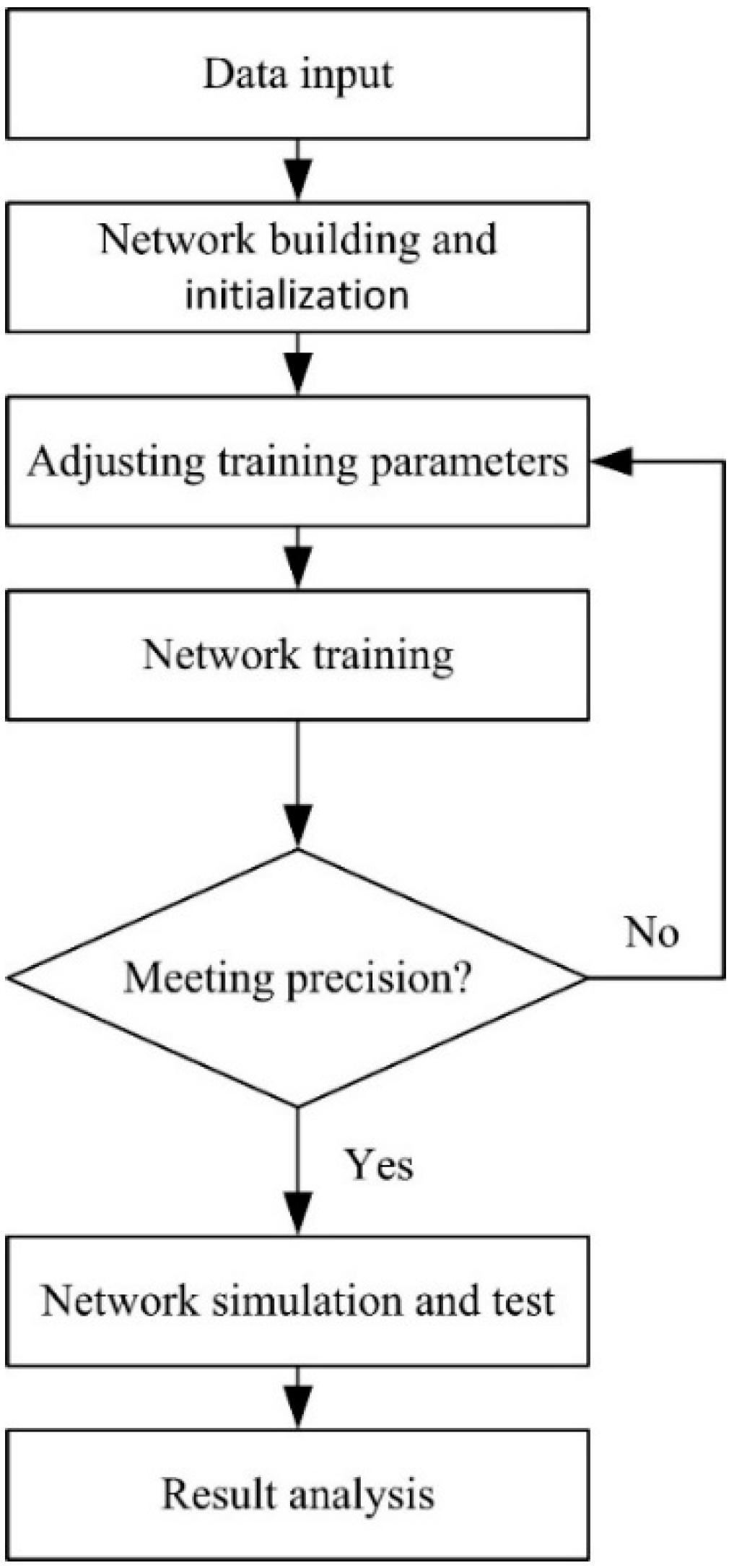
3.2.3. Realization of the Neural Network Model

In this study, Matlab was used to train and realize the neural network model. Two methods can be used to establish a neural network model. One method builds the model through typing the program code into a command window and the other uses the neural network toolbox (nntool) of Matlab.

(1) Importing training and test samples into Matlab

Set the input and output values of the training samples as P and T, respectively, and set the input and output values of the test samples as J and K, respectively.

(2) Create a neural network

a.

Create the BP neural network through calling the function newff

net = newff(PR,[S1 S2...SN],{TF1 TF2...TFN},BTF,BLF,PF)

PR: a matrix with R*2, it comprises the minimum and maximum values of each dimension of R dimension input vectors;

Si: the number of neurons in the i layer;

TFi: the transfer function in the i layer, defaults to tansig;

BTF: the training function, defaults to trainlm;

BLF: the learning function, defaults to learngdm;

PF: the performance function, defaults to mse.

In this study, tansig was chosen as the transfer function from the input layer to the hidden layer, purelin was chosen as the transfer function from the hidden layer to the output layer, the number of nodes in the hidden layer varied from 15 to 20, and the rest of the parameters were set as defaults.

b.

Determine the training parameters of the neural network

Set the network iteration to be 300, set the target precision to be 0.01, and set the learning rate to be 0.05.

c.

Train the neural network model

During the training process, P is set as the input sample and T is set as the output sample. Figure 4 shows a linear regression analysis diagram of the training result and real value when the number of nodes in the hidden layer was 20. The abscissa “Target” represents the real value of the Chl-a concentration and the ordinate “Output” represents the output value of the network training.

d.

Simulation and analysis of the BP neural network model

The test samples were imported, of which J were the input samples and K were the output samples. The “sim” function was called to perform the network simulation test.

$$\mathrm{R}=\text{sim} (\text{net},\mathrm{J})$$

(5)

The difference value was calculated between the real and test values of the test samples, as E = K − R; the “mse” function was called to calculate the mean square error (MSE):

$$\text{MSE}=\text{mse} \left(\mathrm{E}\right)$$

(6)

The best neural network model was selected by comparison of the size of the MSE.

4. Results

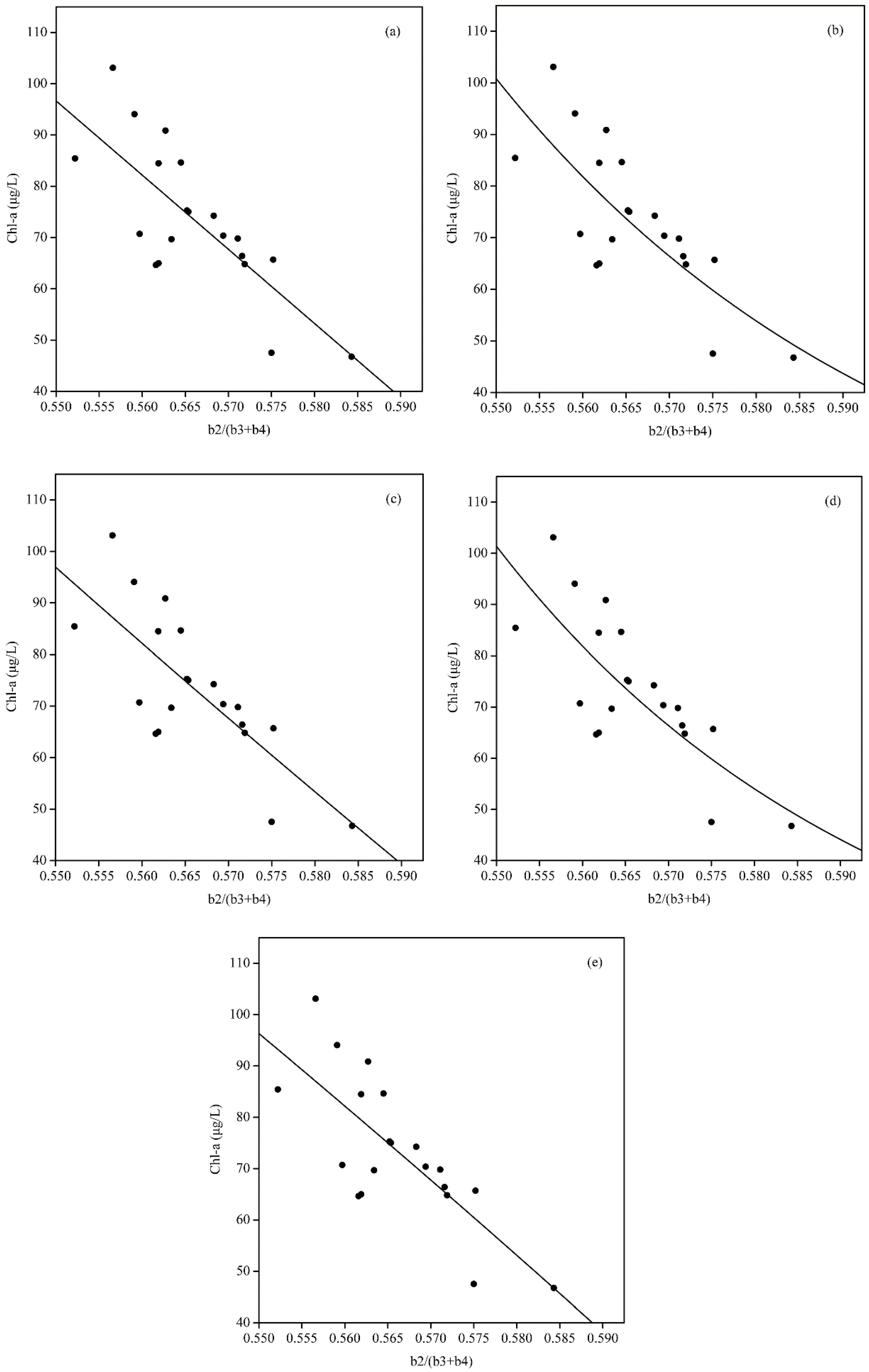
4.1. Results of the MRA Model

The regression models adopted in this study included linear, exponential, logarithm, power, and polynomial models. We used the SPSS software for data regression analysis. It was published by International Business Machines Corporation Inc. (Armonk, NY, USA) in 2010. The results are shown in

Table 1. Regression models of Chl-a concentration based on remote sensing images.

Mathematic Model	Fitted Equation	R-Square
Linearity	y = −1446.933x + 892.461	0.583
Exponent	y = 9921252.875e−20.903x	0.611
Logarithm	y = −820.955 ln(x) − 393.826	0.583
Power	y = 0.085x−11.849	0.610
Polynomial	y = −1274.687x2 + 481.917	0.584

Note: x denotes the ratio of the blue band to the sum of the green and red bands; y denotes the Chl-a concentration.

.

It shows that the value of the R-squared is greatest for the exponential model, followed in order by the power, logarithm, and linear models. The regression curve for each model is shown in Figure 5. As can be seen from the Figure 5, the best-fitted model is the exponential model.

Then the sum of squares due to error (SSE), Adjusted R-squared, and root mean square error (RMSE) were counted, as shown in

Table 2. Analysis parameter of mathematical regression model.

Mathematic Model	SSE	Adjusted R-Square	RMSE
Linearity model	1569.383	0.560	9.337
Exponent model	1631.027	0.590	9.519
Logarithm model	1571.965	0.559	9.345
Power model	1637.414	0.588	9.538
Polynomial model	1567.177	0.561	9.331

. It can be seen that the validation of exponential model has the best result. Four points not involved in the modeling were taken as verification points for a precise evaluation. Considering the exponential model had better fitting effect, we take the exponential model to validation actually. After that, the inversion concentration values from the model calculation were compared with the actual measured concentration values, as shown in

Table 3. Retrieval results and errors of mathematical regression model.

Measured Concentration (μg/L)		118.76	120.66	106.95	55.05
Linearity model	Inversion concentration (μg/L)	78.56	80.15	73.79	69.45
	Absolute error (μg/L)	−40.2	−40.51	−33.16	14.4
	Relative error (%)	−33.85	−33.57	−31	26.16
Exponential model	Inversion concentration (μg/L)	77.65	78.57	72.48	68.07
	Absolute error (μg/L)	−41.11	−42.09	−34.47	13.02
	Relative error (%)	−34.62	−34.88	−32.23	23.65

. After verification, the relative errors of the model were found to be between 0% and 35%.

The Chl-a concentration was inverted using the MRA model and the remote sensing imagery, and the resultant spatial distribution of Chl-a concentration is shown in Figure 6. Through the concentration histogram of Chl-a, it is easy to find that 55 μg/L is the highest probability of the Chl-a concentration. Thus, 55 μg/L was chosen as the classification threshold of Chl-a concentration. Chl-a concentrations of no more than 55 µg/L were placed into one category (shown as green) and Chl-a concentrations more than 55 µg/L were placed into a second category (shown as blue). It can be seen from Figure 6 that the Chl-a concentration of almost the entire study area was more than 55 µg/L.

4.2. Results of the ANN

Through changing the number of nodes in the hidden layer and several further training, the correlations shown in

Table 4. MSE and correlation index of different hidden layer node numbers.

Hidden Layer Nodes Number	15	16	17	18	19	20
MSE	800.1991	559.9822	488.8999	475.8522	460.7343	410.1737
R-square	0.65	0.71	0.74	0.75	0.88	0.94

were obtained. When the number of nodes in the hidden layer was 20, the MSE reached a minimum, R-squared reached a maximum, and the degree of fitting was the best. Therefore, in this study, a BP neural network with three layers and 20 nodes in the hidden layer was adopted as the inversion model for Chl-a concentration. The retrieval results and errors are shown in

Table 5. Retrieval results and errors of the test samples.

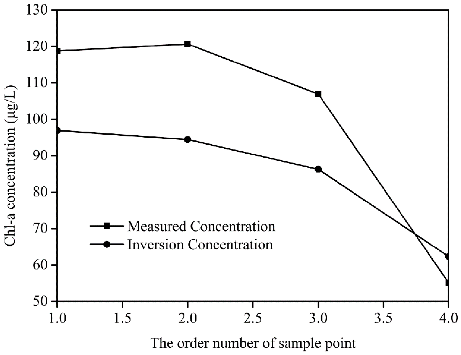
Sample Points Number	Measured Concentration (μg/L)	Inversion Concentration (μg/L)	Absolute Error (μg/L)	Relative Error (%)
1	118.7556	96.9535	21.8021	−18.4
2	120.6582	94.4702	26.1880	−21.7
3	106.9526	86.2942	20.6584	−19.3
4	55.0544	62.3194	7.2650	13.2

.

The inversion ability test of the BP neural network, based on the training and comparison above (Figure 7), produced MSE and R-squared values of 410.17 and 0.94, respectively, which meet the conditions for the required accuracy.

The Chl-a concentration in the study area was inversed using the neural network inversion model and the remote sensing imagery. The reflectance values were extracted from the imagery and input into the completed model. Then, the Chl-a concentration was calculated and the map of the distribution of Chl-a concentration is shown in Figure 8. It can be seen from Figure 8 that the area of Chl-a concentration of no more than 55 μg/L is larger than in Figure 6. Thus, the Chl-a inversion results of the ANN model are shown to be better than the MRA model, indicating that the ANN model is more suited to the inversion of Chl-a concentration in the study area.

5. Discussion

Which band can be selected for the input layer neurons? In this study, this selection was performed by comparing the R-squared of different combinations of bands. As shown in the correlation table, the variation of correlation was not great between combinations of four or five bands to a combination of seven bands; therefore, the required accuracy was achievable by changing the number of nodes in the hidden layer in the late stages. It is recognized that a better selection criterion for the selection of the input layer is required. In this study, the main modification made to the neural network parameters was changing the number of nodes in the hidden layer; the parameters of the transfer function and training function needed little modification. Therefore, establishing a method of parameter selection that better fits the water inversion is another improvement that should be addressed in future work. In this study, the number of samples was insufficient, and some of the sample points were in mixed pixels of the remote sensing images, both of which affected the accuracy and effectiveness of the neural network model.

6. Conclusions

In this study, the section of the Haihe River in the Binhai New Area of Tianjin was chosen as the water study area. The Chl-a concentration of water was measured at a number of sampling points in the field. The reflectance values of the water at the sampling points were retrieved by the OLI sensor onboard the Landsat-8 satellite. A correlation analysis between the Chl-a concentration and reflectance value data acquired at the same time was performed, and MRA and ANN models were built for the inversion of the remote sensing Chl-a concentration. Here, the MRA and ANN models were applied to invert the Chl-a concentration. For the MRA, the ratio of the blue band to the sum of the green and red bands was adopted for use with the linear, exponential logarithm, power, and polynomial regression models. After verification, the relative errors of the model were found to be between 0% and 35%, showing that the precision of the model was not high at certain points. For the ANN model, a BP neural network with three layers and 20 nodes in the hidden layer was selected. In the inversion ability test, the MSE and R-squared values were 410.17 and 0.94, respectively, both meeting the required accuracy. From the aspects of statistical significance, both methods can handle considerable sample data and select an appropriate model. However, the ANN model is more consistent with the mode of human logic, and it demonstrated the highest efficiency and smallest error. Ultimately, the ANN model showed better performance than the MRA model by displaying higher accuracy in the validation.

References

- Boyer, J.N.; Kelble, C.R.; Ortner, P.B.; Rudnick, D.T. Phytoplankton bloom status: Chlorophyll a biomass as an indicator of water quality condition in the southern estuaries of Florida, USA. Ecol. Indic. 2009, 9, S56–S67. [Google Scholar] [CrossRef]
- Wang, Y.; Jiang, H.; Jin, J.; Zhang, X.Y.; Lu, X.H.; Wang, Y.Q. Spatial-temporal variations of Chlorophyll-a in the adjacent sea area of the Yangtze River estuary influenced by Yangtze River discharge. Int. J. Environ. Res. Public Health 2015, 12, 5420–5438. [Google Scholar] [CrossRef] [PubMed]
- Le, C.; Hu, C.; Jennifer, C.; David, E.; Frank, M.-K.; Lee, Z. Evaluation of chlorophyll-a remote sensing algorithms for an optically complex estuary. Remote Sens. Environ. 2013, 129, 75–89. [Google Scholar] [CrossRef]
- Cheng, A.C.; Wei, Y.; Lv, G.; Yuan, Z. Remote estimation of chlorophyll-a concentration in turbid water using a spectral index: A case study in Taihu Lake, China. J. Appl. Remote Sens. 2013. [Google Scholar] [CrossRef]
- Sun, D.Y.; Hu, C.M.; Qiu, Z.F.; Cannizzaro, J.P.; Barnes, B.B. Influence of a red band-based water classification approach on chlorophyll algorithms for optically complex estuaries. Remote Sens. Environ. 2014, 155, 289–302. [Google Scholar] [CrossRef]
- Pan, G.; Tang, D.; Zhang, Y. Satellite monitoring of phytoplankton in the East Mediterranean Sea after the 2006 Lebanon oil spill. Int. J. Remote Sens. 2012, 33, 7482–7490. [Google Scholar] [CrossRef]
- Liu, X.F.; Duan, H.T.; Ma, R.H. The spatial heterogeneity of water quality variables in Lake Taihu, China. J. Lake Sci. 2010, 22, 367–374. [Google Scholar]
- Ma, R.H.; Tang, J.W.; Duan, H.T.; Pan, D. Progress in lake water color remote sensing. J. Lake Sci. 2009, 21, 143–158. [Google Scholar]
- Gómez, J.A.D.; Alonso, C.A.; García, A.A. Remote sensing as a tool for monitoring water quality parameters for Mediterranean Lakes of European Union water framework directive (WFD) and as a system of surveillance of cyanobacterial harmful algae blooms (SCyanoHABs). Environ. Monit. Assess. 2011, 181, 317–334. [Google Scholar] [CrossRef] [PubMed]
- Song, K.S.; Wang, Z.M.; Blackwell, J.; Zhang, B.; Li, F.; Zhang, Y.Z. Water quality monitoring using Landsat Themate Mapper data with empirical algorithms in Chagan Lake, China. J. Appl. Remote Sens. 2011, 5, 944–956. [Google Scholar] [CrossRef]
- Casas, A.; Riaño, D.; Ustin, S.L.; Dennison, P.; Salas, J. Estimation of water-related biochemical and biophysical vegetation properties using multitemporal airborne hyperspectral data and its comparison to MODIS spectral response. Remote Sens. Environ. 2014, 148, 28–41. [Google Scholar] [CrossRef]
- Hunter, P.D.; Gilvear, D.J.; Tyler, A.N.; Willby, N.J.; Kelly, A. Mapping macrophytic vegetation in shallow lakes using the Compact Airborne Spectrographic Imager (CASI). Aquatic Conserv. Mar. Freshw. Ecosyst. 2010, 20, 717–727. [Google Scholar] [CrossRef]
- Wittenberghe, S.V.; Alonso, L.; Verrelst, J.; Moreno, J.; Samson, R. Bidirectional sun-induced chlorophyll fluorescence emission is influenced by leaf structure and light scattering properties—A bottom-up approach. Remote Sens. Environ. 2015, 158, 169–179. [Google Scholar] [CrossRef]
- Thiemann, S.; Kaufmann, H. Determination of chlorophyll content and strophic state of lakes using field spectrometer and IRS-1C satellite data in the Mecklenburg lake district, Germany. Remote Sens. Environ. 2000, 73, 227–235. [Google Scholar] [CrossRef]
- Santos, L.C.M.; Matos, H.R.; Schaeffer-Novelli, Y.; Cunha-Lignon, M.; Bitencourt, M.D.; Koedam, N. Anthropogenic activities on mangrove areas (São Francisco River Estuary, Brazil Northeast): A GIS-based analysis of CBERS and SPOT images to aid in local management. Ocean Coastal Manag. 2014, 89, 39–50. [Google Scholar] [CrossRef]
- Zhang, M.; Hu, C.; English, D.; Carlson, P. Atmospheric correction of AISA measurements over the Florida keys optically shallow waters: Challenges in radiometric calibration and aerosol Selection. IEEE J. Sel. Top. Appl. Earth Obs. Remote Sens. 2015, 8, 1–8. [Google Scholar] [CrossRef]
- Ogashawara, I.; Alcântara, E.; Curtarelli, M.; Adami, M.; Nascimento, R.; Souza, A.; Stech, J.; Kampel, M. Performance analysis of MODIS 500-m spatial resolution products for estimating Chlorophyll-a concentrations in Oligo- to Meso-Trophic waters case study: Itumbiara reservoir, Brazil. Remote Sens. 2014, 6, 1634–1653. [Google Scholar] [CrossRef]
- Stephanie, C.J.P.; Peter, D.H.; Thomas, L.; Steven, H.; Evangelos, S.; Andrew, N.T.; Mátyás, P.; Hajnalka, H.; Alistair, L.; Heiko, B.; et al. Validation of Envisat MERIS algorithms for chlorophyll retrieval in a large, turbid and optically-complex shallow lake. Remote Sens. Environ. 2014, 157, 158–169. [Google Scholar]
- Jiang, G.J.; Zhou, L.; Ma, R.H.; Duan, H.T.; Shang, L.L.; Rao, J.W.; Zhao, C.L. Remote sensing retrieval for chlorophyll-a concentration in turbid case II water (II): Application on MERIS image. J. Infrared Millim. Waves 2013, 32, 372–378. [Google Scholar] [CrossRef]
- Wen, J.G.; Xiao, Q.; Yang, Y.P.; Liu, Q.H.; Zhou, Y. Remote sensing estimation of aquatic chlorophyll-a concentration based on Hyperion data in Lake Taihu. J. Lake Sci. 2006, 18, 327–336. [Google Scholar]
- Mo, D.K.; Yan, E.P.; Hong, Y.F.; Lin, H. Research on the spatial variation of water quality parameters in East Dongting Lake based on Hyperion. Chin. Agric. Sci. Bull. 2013, 29, 192–198. [Google Scholar]
- Monika, W.; Katarzyna, B.; Mirosław, D.; Adam, K. Empirical model for phycocyanin concentration estimation as an indicator of cyanobacterial bloom in the optically complex coastal waters of the Baltic Sea. Remote Sens. 2016, 8, 212. [Google Scholar]
- Huang, Y.H.; Jiang, D.; Zhuang, D.F.; Fu, J.Y. Research on remote sensing estimation of chlorophyll concentration in water body of Tangxun Lake. J. Nat. Disasters 2012, 21, 215–222. [Google Scholar]
- Carder, K.; Chen, F.R.; Cannizzaro, J.P.; Campbell, J.W.; Mitchell, B.G. Performance of the MODIS semi-analytical ocean color algorithm for chlorophyll-a. Adv. Space Res. 2004, 33, 1152–1159. [Google Scholar] [CrossRef]
- González, L.; Spyrakos, E.; Torres, J.M. Neural network estimation of chlorophyll a from MERIS full resolution data for the coastal waters of Galician Rias (NW Spain). Remote Sens. Environ. 2011, 115, 524–535. [Google Scholar] [CrossRef]
- Chen, J.; Wen, Z.H.; Fu, J. The application of the subsection mapping retrieval model to water qualities quantitative analysis. Spectrosc. Spectr. Anal. 2010, 30, 2784–2788. [Google Scholar]
- Giardino, C.; Brando, V.E.; Dekker, A.G.; Strömbeck, N.; Candiani, G. Assessment of water quality in Lake Garda (Italy) using Hyperion. Remote Sens. Environ. 2007, 109, 183–195. [Google Scholar] [CrossRef]
- Chen, J.; Quan, W.; Wen, Z.; Cui, T. An improved three-band semi-analytical algorithm for estimating chlorophyll-a concentration in highly turbid coastal waters: A case study of the Yellow River estuary, China. Environ. Earth Sci. 2013, 69, 2709–2719. [Google Scholar] [CrossRef]
- Park, Y.; Cho, K.H.; Park, J.; Cha, S.M.; Kim, J.H. Development of early-warning protocol for predicting chlorophyll-a concentration using machine learning models in freshwater and estuarine reservoirs, Korea. Sci. Total Environ. 2015, 502, 31–41. [Google Scholar] [CrossRef] [PubMed]
- The state environmental protection administration. Water and Exhausted Water Monitoring Analysis Method; China Environmental Science Press: Beijing, China, 1997. (In Chinese) [Google Scholar]
- Nan, J.H. Research on Decision Neural Network Model with Applications; Huazhong University of Science and Technology: Wuhan, China, 2008. (In Chinese) [Google Scholar]
- Zhang, B.; Li, J.S.; Wang, Q.; Shen, Q. The High Spectral Remote Sensing of Inland Water; Science Press: Beijing, China, 2012; pp. 186–187. (In Chinese) [Google Scholar]
- Ressom, H.; Miller, R.L.; Natarajan, P.; Slade, W.H. Computational intelligence and its application in remote sensing. Remote Sens. Coast. Aquat. Environ. 2005, 7, 205–227. [Google Scholar]