1. Introduction
The carbon cycle system and its mechanism are the main contents of the Global Change and Terrestrial Ecosystem (GCTE), as well as many other core research plans in the International Geosphere-Biosphere Program (IGBP). The terrestrial carbon cycle is the most important constitution and plays the prominent position in the global carbon cycle.
The research on the terrestrial carbon cycle establishes the foundation of the prediction of atmospheric levels. Measuring the level of the carbon source and sink is not only helpful for understanding the evolution, but also offering the theoretical basis for the regulation and control of global climate change. It also contributes to the economic and social development strategy and environmental diplomatic policy for all countries.
Regarding China’s regional terrestrial ecosystem carbon system, establishing China’s regional carbon cycle evolution model will contribute to the identification of China’s regional carbon cycle system state, the analysis of the terrestrial carbon cycle mechanism, as well as policy making for carbon emission. The research shows in detail the exchange process of China’s regional carbon sink/source and its influence. It helps to understand the interaction and relationship of various factors and the impact of human activities, as well as to maintain the continuous and stable development of the terrestrial ecosystem by regulating human activities and adjusting the carbon cycle system. Therefore, it is important to study the features, structure and evolution of China’s regional carbon cycle and carbon balance in order to realize the sustainable development of China’s regional ecological environment system.
2. Literature Review
A great number of theoretical issues concerning the carbon cycle have been studied in many fields, i.e., geological sciences, geosciences, atmosphere science, ocean science, energy development and utilization of science from the perspective of terrestrial ecosystems, marine ecosystems and forest ecological systems. Research achievements mainly concentrate on the carbon source and sink, carbon footprint and carbon exchange. Most of them are related to professional techniques. This study establishes a dynamical model to analyze the evolution of the carbon cycle.
Michela
et al. [
1] established a carbon cycle dynamic model for Italy, Siena province, and examined the carbon footprint of six carbon emission scenarios. Leonid
et al. [
2] built a terrestrial ecosystem carbon life cycle model to study the intensity of carbon source and sink. Strhbach
et al. [
3] used the life cycle approach to survey the carbon footprint of urban green space. Pan
et al. [
4] assessed the global forest carbon balance. Luo
et al. [
5] proposed a dynamic imbalance framework on the terrestrial ecosystem carbon cycle, which has been used to forecast the dynamic process of the terrestrial carbon sink in the future. It was found that internal ecosystem processes will develop toward balance. Mattila
et al. The work in [
6] proposed a question of whether biology or straw constitutes a good carbon sink. Then, the generation and influence of biology and straw carbon are compared. Alexey
et al. [
7] used a conceptual linear coupling model to explain the ultimate saturability of climate-carbon cycle feedback. Andrew
et al. [
8] explained the relationship of weathering and the global carbon cycle from the view of the landform.
Enting [
9] proposed the Laplace transform of carbon cycle analysis. Churkina [
10] believed biophysical and human-related carbon flux should be added into the city carbon cycle model according a survey. Jackson
et al. [
11] integrated the carbon cycle, human activities and the climate system and examined the extent of carbon-climate feedback. King
et al. [
12] proposed a carbon cycle model, which is able to examine the sensitivity of the carbon cycle to climate and location factors. Nusbaumer
et al. [
13] studied the variation of climate and the carbon cycle under the critical situation. Joyita
et al. [
14] built a seven-dimension carbon cycle dynamic model for Hooghly-Matla region of India. They discussed the carbon cycle pattern and conversion mechanism of different carbon forms.
Wang
et al. [
15] discussed the necessity to start research on China’s regional terrestrial ecosystem carbon balance. Yu
et al. [
16] proposed the technical approaches and measures to control the balance of the regional ecosystem carbon budget. Piao
et al. [
17,
18] firstly used a bottom-up atmospheric inversion model and a bottom-up process model, combing remote sensing data and a biogeochemical model, to describe China’s carbon budget and its change mechanism. Fang
et al. [
19] analyzed China’s grassland ecosystem carbon library and its dynamic change. Huang
et al. [
20] discussed the issues of China’s soil carbon reserve change, land utilization variation, the carbon source and sink effect and measures and estimations for deep soil organic carbon change. Luo
et al. [
21] studied the influence of different factors on the soil carbon cycle,
i.e., the land utilization change during urbanization, management of soil and organisms, urban microclimates, atmospheric pollution settlement and soil pollution. Geng
et al. [
22] analyzed the important issue of premise-border demarcation in carbon footprint assessment. Yang [
23] raised some recommendations on land resource management in order to reduce carbon emissions and realize a low carbon economy. Zhao
et al. [
24] explored the general characters of the city carbon cycle system and proposed an analysis framework based on system level division and the carbon circulation process. Li
et al. [
25] reviewed and summarized the key factors that influence the forest-soil carbon cycle. Lun
et al. [
26] studied the influence of the biological cycle and the industrial cycle on the forest carbon cycle and proposed measures for carbon emission reduction. He [
27] explored China’s carbon cycle of the forest ecological system from the viewpoint of the reserve, dynamics and development pattern.
Qin
et al. [
28] built a coupling model of a regional carbon cycle and water cycle, which is used to study the endogenous factors and dynamic mechanism of the carbon cycle and water cycle system. Li
et al. [
29] compared various analogies and statistical approaches of the atmosphere carbon cycle. Tao
et al. [
30] presented the characteristics of different carbon pools, including the atmosphere, marine and terrestrial ecosystems. Liu
et al. [
31] studied the variation and spatial distribution of the wetland soil organic carbon of different climate zones in China. Fan
et al. [
32] explored the impact of climate warming on the grassland ecosystem carbon cycle. Huang
et al. [
33] built a carbon emissions model and carbon sequestration model based on regional human activities and established a carbon cycle pressure index model.
Jing
et al. [
34] surveyed the environmental control and secular change of the carbon cycle of oak temperate forest. Yang
et al. [
35] proposed the health threshold of carbon storage within a balance model of land, water, nitrogen and carbon cycle. Li
et al. [
36] built an eight-procedure mass balance equation to examine the evolution and long-term equilibrium mechanism of the carbon cycle in the past one hundred million years.
Based on the above analysis, the existing literature has provided a solid empirical investigation and a good reference for understanding the carbon cycle system, but some problems still need to be further examined. Firstly, there are no obvious strides in the research of China’s regional terrestrial ecosystem carbon source/sink and conversion mechanism. The function of the terrestrial carbon cycle system in the global carbon cycle is uncertain. Secondly, it is believed that the function of the terrestrial carbon cycle system in reducing concentration in the atmosphere is very important. Existing studies have linked the terrestrial atmospheric carbon flux with international politics and the economy. Therefore, it is urgent to build a credible terrestrial-atmospheric carbon flux exchange model for China. The carbon cycle is a complex dynamic changing process. Former studies mainly used the methods of scenario analysis, and the result is not desirable, because of too many uncertain factors. The evolution of the carbon cycle is not clear yet. There is still a lack of studies using a non-linear dynamic approach to research the evolution of the carbon cycle. Therefore, it is necessary to build a nonlinear carbon cycle evolution model based on the understanding of the complex relationship among atmosphere, soil and land, in order to study the evolution law systematically by using non-linear dynamic theory.
Different from the previous research, this paper uses nonlinear dynamics theory and nonlinear differential equation theory to put the atmosphere, soil and land cycle into a nonlinear system to analyze. This study will establish a regional dynamic desalination system model to examine the carbon flow of the regional atmosphere-soil-land cycle and exploring the desalt law of each carbon cycle. Moreover, we will study the dynamic law of systematic changes with time and apply our model to study the changes of the carbon cycle of Nanjing region in China.
The paper is organized as follows. The regional carbon cycle power system is established in
Section 2.
Section 3 is devoted to a dynamics analysis.
Section 4 is model initialization.
Section 5 carries out a numerical simulation of the Nanjing case.
Section 6 concludes the study with some recommendations.
3. The Construction of the Model
We use to indicate the carbon flux with time t in the regional atmosphere. Variable is the carbon flux of regional soil. Variable is the carbon flux of regional animals and plants. Variable is the carbon inflows into cycle i of the outside and is outflows of cycle i. The flow function is the internal carbon flow from cycle i to cycle j, i, j = 1, 2, 3, where 1 is the regional atmosphere cycle, 2 is the regional soil cycle and 3 is the regional animals and plants’ cycle.
Based on the law of regional carbon flow, we propose the following assumptions:
Hypothesis 1: the balance of regional carbon flow of the inside and outside follows the rule of:
where inflow
q and outflow
f equal the total regional carbon flow
y.
Hypothesis 2: the regional internal carbon flux is determined by the carbon flow of three cycles (atmosphere cycle, soil cycle and animals and plants’ cycle) in the region.
where
indicates the carbon flow from cycle
k to
i and
is the carbon flow from cycle
i to
k.
Hypothesis 3: carbon inflow is not dependent on a responding corresponding carbon reserve. Therefore, it could be considered as a constant number or time-varying function,
Hypothesis 4: the carbon outflow is positive correlated with the carbon inflow of the cycle.
where
is the carbon inflow of cycle
i at the beginning. Normally,
. Therefore,
Hypothesis 5: the internal flow of each cycle in the region obeys the following three rules.
(a) Supply pattern: carbon flow
has a linear relationship with carbon reserve
,
(b) Receive pattern: carbon flow
depends on the receiver’s carbon reserve
,
(c) Lotka–Volterra pattern: carbon flow
depends on the carbon reserve of cycle
k and cycle
i,
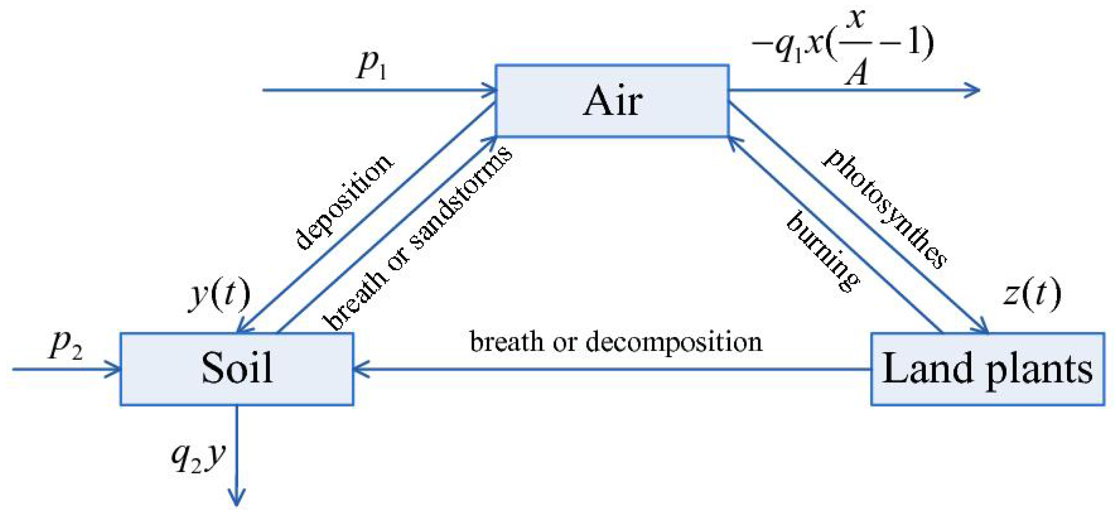
Based on Hypothesis 1–5, we could build the regional atmosphere-soil-land terrestrial ecosystem carbon cycle dynamic model as shown in
Figure 1.
In such regions, we assume the carbon inflow of the atmosphere cycle is constant. The carbon inflow of the land cycle is also constant.
As shown in
Figure 1, a part of carbon flow
of the atmosphere cycle escapes out of the region with the change of wind and temperature, except
. Some of
sinks into the land cycle
, while some of it flows into the animal-plant cycle
. In the solid cycle, a part of carbon flow
goes into the atmosphere cycle by the respiration of the sand, ground or the grass, while another part
goes out of the region with water flow. In the animal-plant cycle, a part of carbon flow
goes into the atmosphere cycle by combustion and breathing; another part
flows into the solid cycle by excretion and plant roots’ absorption, and the other part leaves the region.
Based on the hypothesis, we have:
where
are positive constant.
Now, we can get the evolution of the dynamic system of the regional carbon cycle as follows:
where
and
are positive constants and
are constants.
A simplified formula is as:
where:
The stability analysis of System (1) is given in the
Appendix. The results of the theoretical analysis of the stability of System (1) indicate that the changes of the parameters in the atmosphere-soil-land cycle system will make the system exist in different states, which shows the complexity of the relationships among the atmosphere cycle, soil cycle and land cycle. It also shows the controllability of the relationship, as the states of the atmosphere-soil-land cycle system can be controlled by adjusting the parameters of the system.
In fact, based on the carbon flux relationship among the atmosphere cycle, soil cycle and land cycle, from
Figure 1 and System (1), we can obtain the equivalent form of System (1),
System (1) and System (2) can both reflect the interactive relationships among the atmosphere cycle, soil cycle and land cycle. In the evolutionary process of both systems, there are complex dynamic characteristics existing between the variables and parameters of both systems. The dynamic evolution characteristics of System (2) were obtained by using numerical simulation methods.
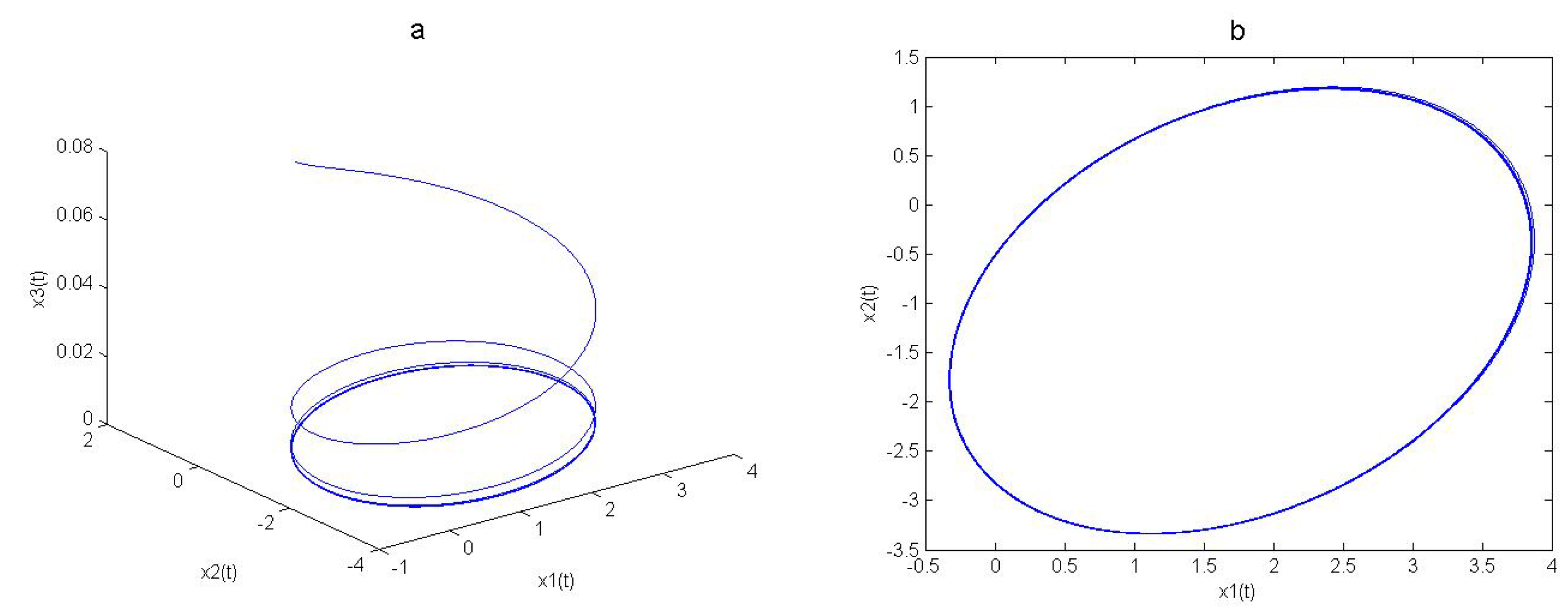
We choose a set of parameters of System (2) as follows:
,
,
; set initial conditions as (0.5,0.2,0.08); a limit cycle can be observed in the system, as shown in
Figure 2a,b. Let
; fix the other parameters as the above; the orbit of the atmosphere-soil-land cycle system is stable at the point, as shown in
Figure 3a,b.
The numerical simulation results show that there is a rather complex nonlinear relationship among the atmosphere cycle, soil cycle and land cycle. It is closely related to the parameters in the model. These models will appear in different values, periods and backgrounds, which will lead to the periodically changing states (
Figure 2) and the stable state (
Figure 3) of the system. Therefore, for an actual system, we can identify the states that the system will finally reach according to the range of the parameters. If the system will be in a chaotic state, thus certain measures need to be taken to adjust the value of the parameter, making the system remain in a steady state. If we can find the means to control the values of the corresponding parameters according to the actual meaning of the parameters, we can carry out an evolutionary analysis with the various effects of regulation on the state of the system.
4. Parameter Estimation Based on the Neural Network Method
The interaction of different carbon cycle is complex. We use Model (1) to describe such relationships. Due to a large number of system parameters, we choose the neural network BP algorithm to identify the system parameters. The BP algorithm has the advantage of low error. For convenience, we choose Nanjing city as the object region of the empirical study. The objective is to obtain the evaluation law of the carbon cycle system of Nanjing region.
4.1. Discretization and Parameters Identification
Firstly, we discretize the three-dimensional regional carbon cycle system and get the differential equations as:
The carbon emissions statistics of Nanjing city are given by
Table 1. Then, we identify the parameters of
in Equation (3). We use data of 2000∼2005 as the input and the data of 2005∼2009 as the output, then normalize the data with following formula,
where
is the input data,
is the minimal value of
and
is the maximal value of
. After normalization, we use the average value as the input and output of the neural network.
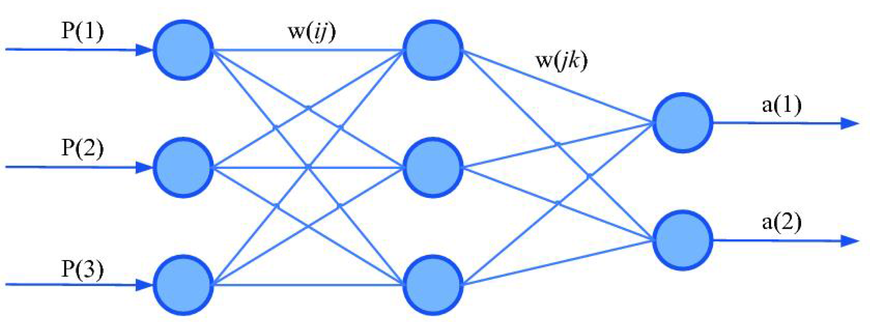
Secondly, we use an appropriate feedforward neural network, as shown in
Figure 4, and set the value of weights and thresholds as random numbers.
We assume is the output layer, l is the hidden layer, is the output layer and n indicates the training. The calculation process is as follows:
(1) Feed-forward calculation:
Regarding the j unit of the layer, it satisfies , where is the working signal sent by unit i of the former input layer. The action function of unit j is an S-type transfer function, . The output of the hidden layer is , which is at the same time input of the output layer.
The same as for the above process, the output of the output layer is
. Substituting the result into differential Equation (3), we get the error
e between result and the target output, as well as:
(2) Back-forward calculation:
For the output unit: .
For the unit of the hidden layer: .
The modifier formulas for weights: .
The modifier formulas for thresholds: , where η is the learning rate, is the amount of weight change and is the amount of threshold change.
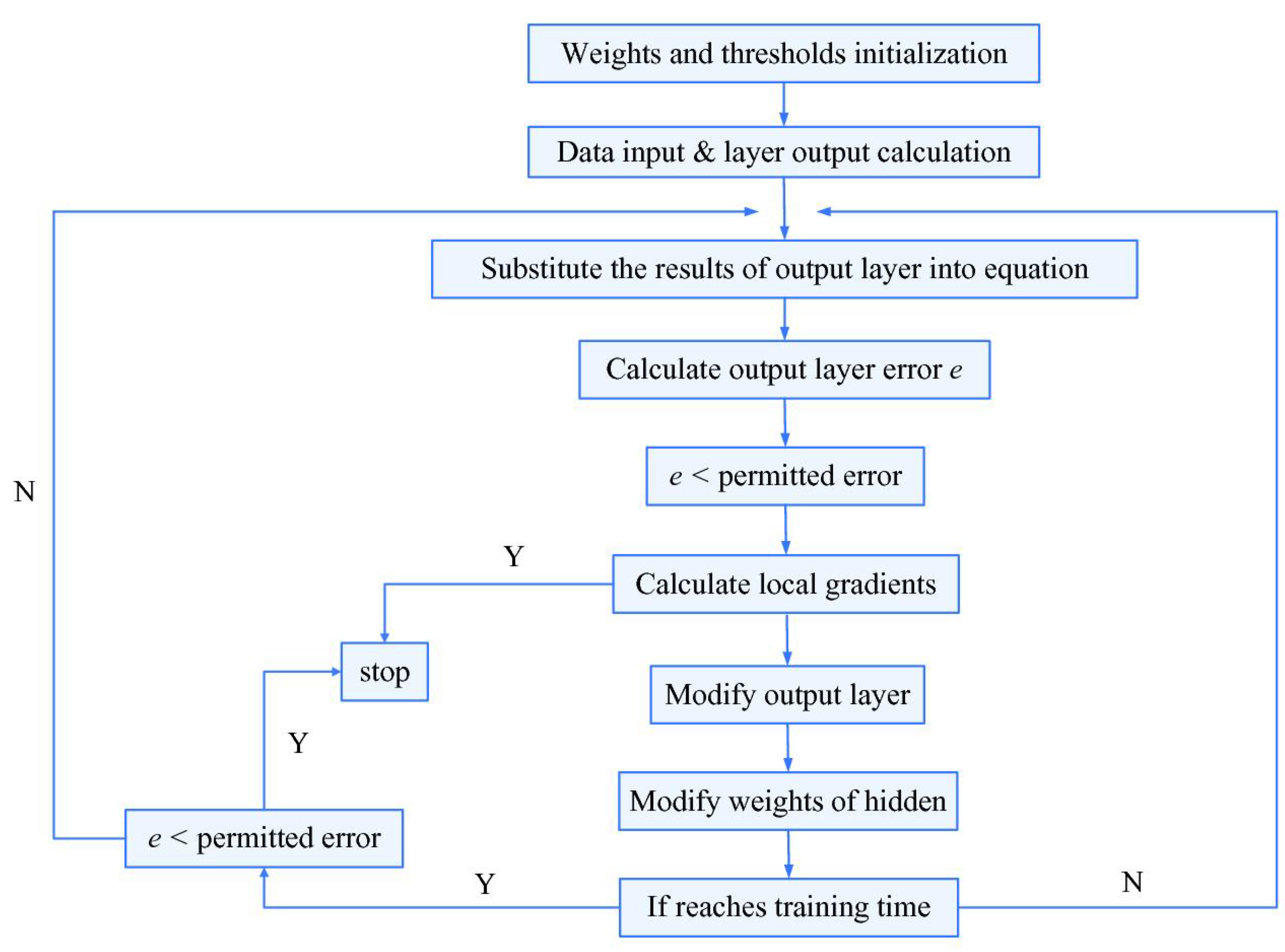
The flow chart for the BP neural network program, as shown in
Figure 5.
The error is set less than
. By multiple iterations, we get the parameters for the Nanjing carbon cycle evolution system, which has been shown in
Table 2.
Therefore, the evolution system is as:
5. Dynamics Analysis for the Nanjing Carbon Cycle Evolution System
5.1. Equilibrium Point
System (4) has the equilibrium point of , , , , .
(1) For equilibrium point , the eigenvalues of its linear approximation system are , , . Therefore, System (4) is stable at . This means that the carbon flux of the atmosphere cycle, soil cycle and animals and plants’ cycle around point is stable.
(2) For equilibrium point , its eigenvalues of the linear approximation system are , , . Thus, is unstable. This means that, around point , the carbon flow of the atmosphere cycle is unstable, while the carbon flow of the soil cycle and animals and plants’ cycle is stable. Therefore, part of the system is unstable.
(3) For equilibrium point , its eigenvalues of the linear approximation system are , , is unstable. The condition is the same as .
(4) For equilibrium point , its eigenvalues of linear approximation system are , , . is stable. The condition is the same as .
(5) For equilibrium point , its eigenvalues of the linear approximation system are , is unstable. This means that, around point , the carbon flow of the atmosphere cycle and animals and plants’ cycle is unstable, while the carbon flow of the soil cycle is stable.
To sum up, there are complex dynamic characteristics existing in the Nanjing carbon cycle evolution system. There are two stable points and three unstable points in the system, and this system will appear to have different states in different backgrounds. Therefore, we can use this system to simulate the evolution track of the carbon cycle in Nanjing city.
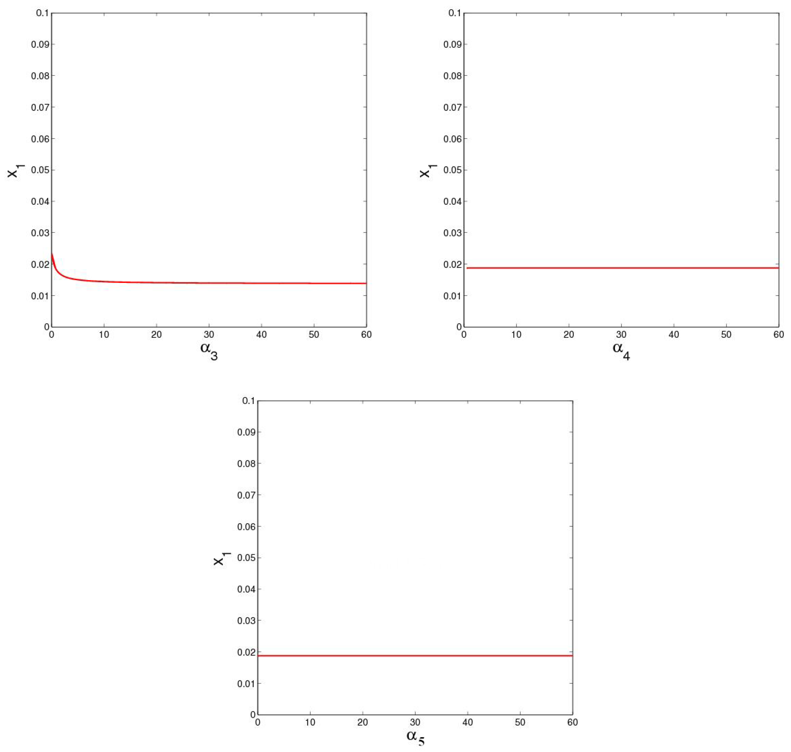
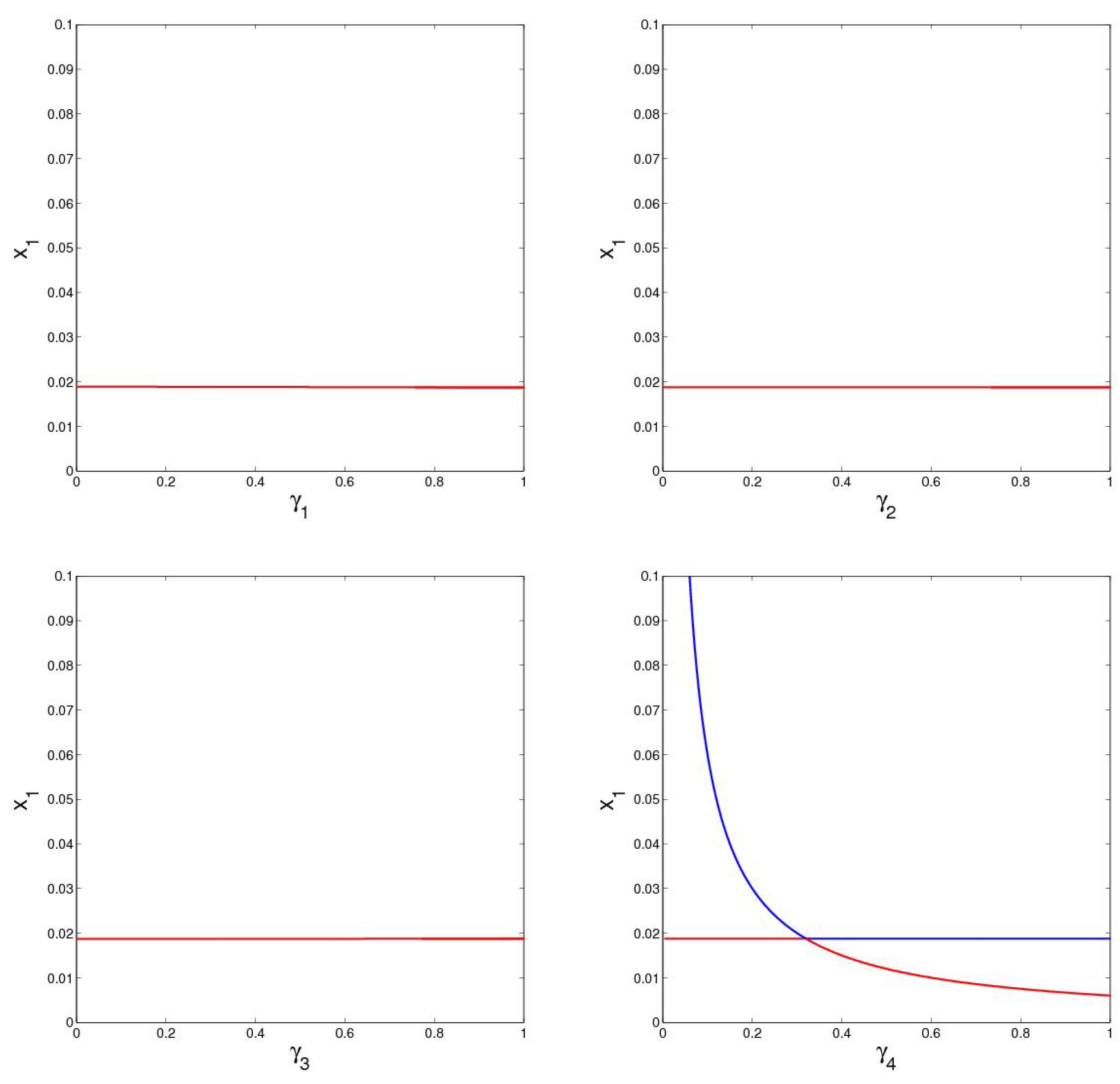
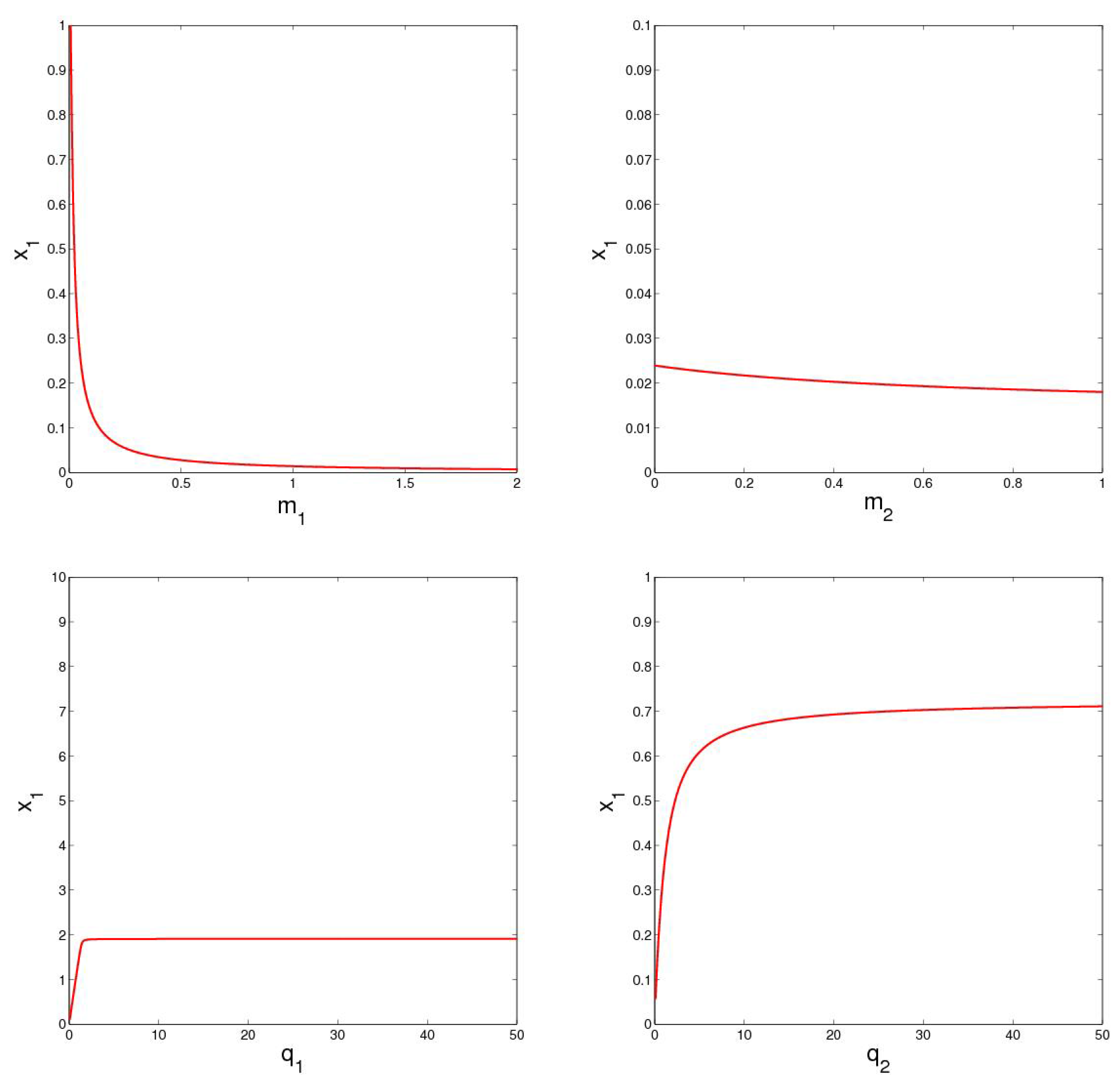
5.2. Bifurcation Analysis for a Single Parameter
From
Figure 6,
Figure 7 and
Figure 8, it is worth noting that the red line indicates stable fixed points and the black line indicates unstable fixed points.
To begin with the single parameter bifurcation of
while others keep constant, as shown in
Table 2, we find the system has a stable fixed point and an unstable fixed point when
varies from 0–51.16. These two points converge at the point of 51.16, which means there is no fixed point when
is larger than 51.16.
Regarding the single parameter bifurcation of , we find the system has a stable fixed point with the increasing of , and the point is constant. This means the variation of has no influence on the fixed point of the system.
Regarding the single parameter bifurcation of , we find the system has a stable fixed point with the increasing of , and the point is constant. This means the variation of has no influence on the fixed point of the system.
Regarding the single parameter bifurcation of , the system has one stable fixed point. With the increasing of , the point decreases slightly at the beginning and becomes stable later.
Regarding the single parameter bifurcation of , the system has a stable fixed point with the increasing of , and the point is constant. This means the variation of has no influence on the fixed point of the system.
Regarding single parameter bifurcation of , the system has a stable fixed point with the increasing of , and the point is constant. This means the variation of has no influence on the fixed point of the system.
Regarding the single parameter bifurcation of , the system has a stable fixed point with the increasing of , and the point is constant. This means the variation of has no influence on the fixed point of the system.
Regarding the single parameter bifurcation of , the system has a stable fixed point and an unstable fixed point. When = 0.3203, the stable fixed point becomes unstable and the unstable fixed point becomes stable.
Regarding the single parameter bifurcation of , the system has one stable fixed point. With the increasing of , the value of the fixed point decreases quickly.
Regarding the single parameter bifurcation of , the system has one stable fixed point. With the increasing of , the point decreases slightly at the beginning and becomes stable later.
Regarding the single parameter bifurcation of , the system has one stable fixed point. With the increasing of , the fixed point increases significantly at the beginning and becomes stable later.
Regarding the single parameter bifurcation of , the system has one stable fixed point. With the increasing of , the fixed point increases significantly at the beginning and becomes stable later.
The above results show that the states of the Nanjing carbon cycle evolution system are closely related to the parameters in System (4). The change of the values of some parameters, such as , will lead to the change of the state of the system, but some parameters, such as , do not. In practice, the model parameters can correspond to the actual policy; the evolution results of the actual system can help to investigate the influence of various regulatory policies on the variables in the systems and to analyze the strength and weakness of these policies quantitatively.
5.3. Numeric Simulation Results and Analysis
This section simulates the carbon cycling system of Nanjing by substituting actual data in System (4). Based on the data given in
Table 1, we choose the average value of the first nine years as the input, (x, y, z) = (0.4809, 0.343, 0.7796). As shown in
Figure 9, the carbon reserve of the atmosphere increases to a maximum value with time, then decreases to a stable level; the carbon reserve of the soil increases to a maximum value with time and then keeps steady; and the carbon reserve of the land cycle decreases to a minimal level and then keeps steady.


