Article

Analyzing Economic Effects with Energy Mix Changes: A Hybrid CGE Model Approach

1
Decommissioning Engineering Team, Decommissioning & Spent Fuel Technology Center, KHNP Central Research Institute, 70, 1312-gil, Yuseong-daero, Yuseong-gu, Daejeon 34101, Korea
2
Division of Future Growth Strategy Research, Korea Economics Research Institute, 24, Yeoui-daero, Yeongdeungpo-gu, Seoul 07320, Korea
3
Department of Industrial and Information Engineering, Yonsei University, 50, Yonsei-ro, Seodaemun-gu, Seoul 03722, Korea
*
Author to whom correspondence should be addressed.
Sustainability 2016, 8(10), 1048; https://doi.org/10.3390/su8101048
Submission received: 8 September 2016 / Revised: 4 October 2016 / Accepted: 11 October 2016 / Published: 19 October 2016
(This article belongs to the Section Energy Sustainability)

Abstract

:
We evaluate the micro and macro-economic effects with the hybrid mixed complementary approach we design to take account of these unique features of the Korean electricity industry. The features we consider are not only the electricity itself but also the Korean electricity market mechanism. Unlike typical commodities, the electricity has unique features. As well known, the electricity supply is not easy to meet an instant hike of rump sum demand of electricity in a smooth and timely manner, since the quantity of power generating is fixed at specific time with the limited capacities. On top of that, we add the Korean electricity market mechanism that the selling price through the Korea Power Exchange (KPX) is unitary, although the marginal production cost of each generating technology. From the modeling point of view, we segment the Korean electricity industry into nine generating technologies such as six conventional and three renewable technologies. In addition, we construct the specifically defined 40-by-40 SAM table to include electricity generating sectors by different resources. With these assumptions, four scenarios for policy simulation are designed according to the supply share reduction of the nuclear power generation. The research result shows micro and macro-economic indices are negatively impacted especially in cases that the share of nuclear power is lower than that of basis case.

1. Introduction

The accident of the nuclear power plant hit by a natural catastrophe in Fukushima has cooled down the attractiveness of nuclear energy mainly due to much tighter security and safety standards incurring far higher reinforcement costs. For instance, many countries whose electricity generation is dominated by nuclear power such as Germany and Switzerland have already announced plans to phase out or shut down their operating reactors from 2022 to 2034. Nonetheless World Energy Outlook [1] published by International Energy Agency (IEA) forecasts electricity generation capacities from the nuclear power worldwide would still steadily increase from 2620 billion kilowatt-hours in 2010 to 5492 billion kilowatt-hours in 2040. According to IEA, the reasons of continuous growth of the nuclear power are concerns about energy security and green-house gas emissions as well as the increasing dependence on the nuclear power in emerging economies such as China, India, Russia and South Korea and the like.
As Korea has focused on nurturing export oriented industries such as heavy chemicals, steel, electric and electronic equipment, which need considerable energy use, the energy intensity (total primary energy supply per unit of GDP) is approximately 1.3 times higher than the average OECD (Organization for Economic Co-operation and Development) countries [2]. Accordingly, Korea is ranked as the tenth energy consumption country in the world. In addition, the lack of natural resources in Korea has led to choose the nuclear power to supplement the continuously increasing energy demand.
The main issue we examine in this paper is to test how much degree of impact gives of increment on Korean economy from the approach of the comparative static analysis, if the nuclear power share would be curtailed to 29% in 2035 according to the Second National Energy Plan issued on 10 December 2013 from 41% in 2030 by the First Energy Plan issued on 27 August 2008.
For methodology we use the hybrid mixed complementary approach [3] by adjusting the integrated top-down and bottom-up model to consider the unique features of electricity itself and the characteristics of the Korean electricity industry. In addition, our model can be classified as a sequential dynamic model which calculates economic effects annually in a static manner.
The organization of this paper is as follows. In Section 2, we explain the concept of a CGE model and the model structures demonstrated by each economic agent of the Korea electric power market. Section 3 explains how input data and parameters are prepared and calibrated. In Section 4, we figure out the illustrative empirical results of each scenario. In Section 5, we reach a conclusion.

2. CGE Model for the Electricity Industry

2.1. Computable General Equilibrium (CGE)

While numerous economic subjects exist as correlated by mutual economic trades in the market, each economic subject tends to behave in order to maximize its payoff; a household gains income by selling its production factors such as labour and capital and tries to maximize its benefit by consuming at the present period or by saving for future expenditure. On the other hand, a corporation produces wealth at the minimum cost by purchasing production factors from households and maximizes its profit by selling or exporting goods to final-consumers and intermediate-consumers. Walrasian General Equilibrium model suggests that the state of equilibrium theoretically exists with maximized social welfare when an economic subject behaves to maximize its own profit and benefit. The equilibrium formed in the market guarantees the optimal social welfare which is the crucial concept of General Equilibrium theory.
Computable General Equilibrium (CGE) model was initially developed by Johansen [4], Harberger [5,6] and Scarf [7,8] on the basis of the theory of General Equilibrium. It is largely used to induce quantitative economic effects against policy changes with the real data such as an input-output table excluding probabilistic assumptions. Due to this feature, CGE model has been broadly applied to areas such as finance, international economics, environmental economics and the theory of economic changes. CGE model has been developed for objectives and usages such as the static general equilibrium model to analyze the static economic state of a specific year, and the sequential static general equilibrium model to evaluate economic effects year by year, and then the balance growth general equilibrium model which is a dynamic model based on the theories of neoclassical economists to calculate the grand total effect at once during the target evaluation period [4,9,10].

2.2. Unique Features of the Korean Electricity Industry
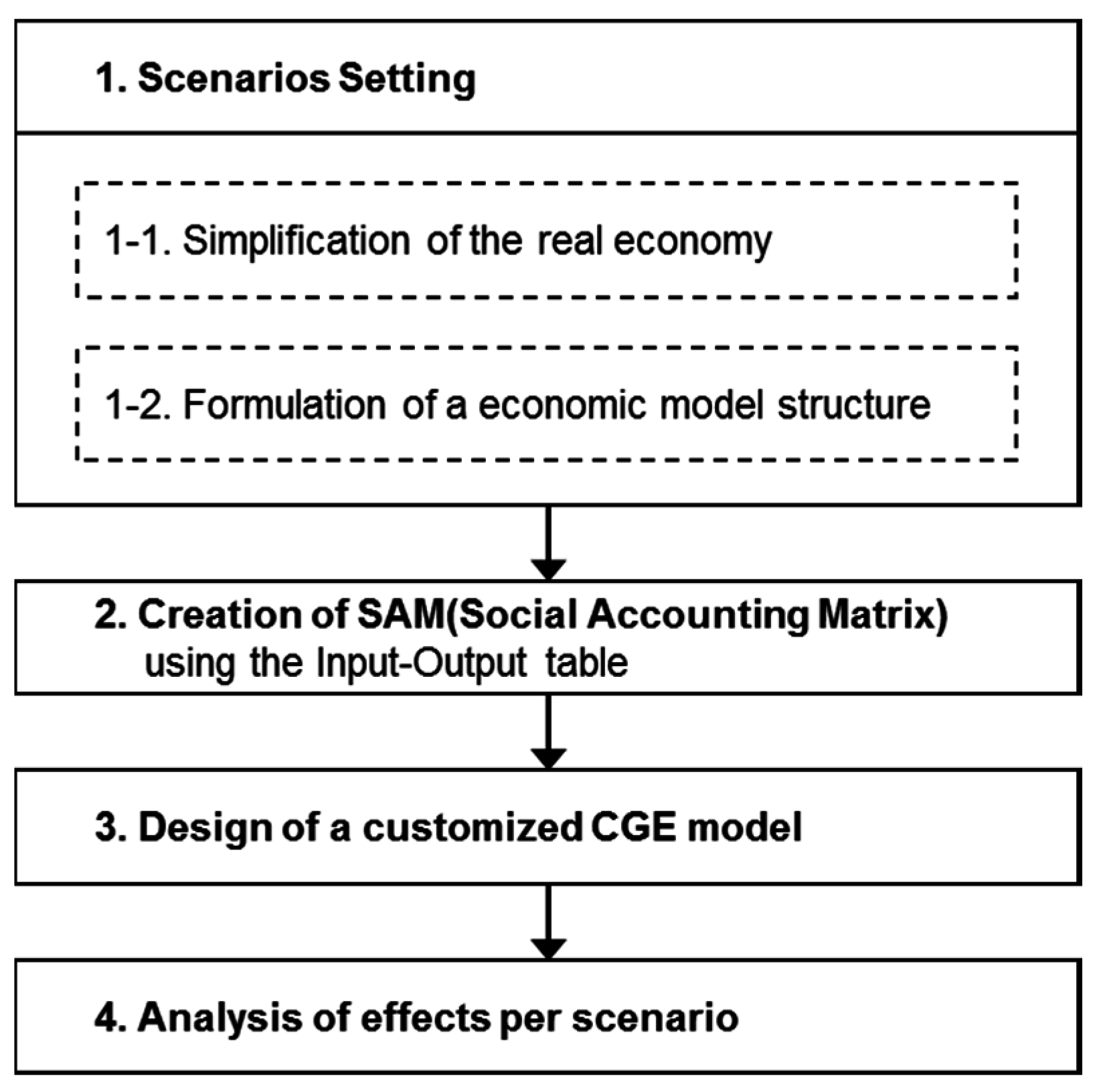
Unlike typical commodities, the electricity has unique features. As the quantity of power generating is fixed at specific time with the limited capacities, it is not easy to meet an instant hike of rump sum demand of electricity in a smooth and timely manner. Because it takes at least 3–5 years to build gas and coal power plants and approximately 10 years in the case of nuclear power plant. In addition, the electricity should be consumed as soon as it is produced due to expensive storage costs. These features make the electricity produced in a trajectory of a step production function. Hence, conventional top-down models such as CGE model could violate fundamental physical characteristics in examining economic effects from energy policy changes. Furthermore, we include the feature of the Korean electricity industry; the selling price through the Korea Power Exchange (KPX) is unitary, although the marginal production cost of each generating technology varies and an offering price from each power generating source to KPX is higher or lower than marginal production cost. As a consequence, offering prices of nuclear and coal plants, in fact, are lower than those of LNG, oil, hydro and renewable power plants. Hence, we designed the hybrid CGE model to take account of these unique features of the Korean electricity industry. We resolve these price discrepancies by the measure of cross subsidy among power generation technologies.

2.3. Model Overview

There are largely two kinds of energy related economic modeling approaches; first, bottom-up energy system models; MARKAL are mainly suitable to resolve partial equilibrium representations of the energy sectors [11]. The objective of these types of models is to feature a larger number of discrete technologies considering the condition of energy producing technologies on the primary and final energy level, process substitution, command and control policies for efficiency improvements and energy savings. As these models are specialized in optimization problems with least cost approach to meet given energy demand, they would often encounter fundamental shortcomings such as a corner solution problem and moreover quite often ignore interaction and feedback with the rest of the economy.
On the other hand, the main purpose of the top-down models is to examine the broader economic framework in consideration of feedback effects between different economic agents when changes of energy policy are needed. Contrary to the bottom-up models, they do not demonstrate technological details of each energy system. Both the energy sectors and the non-energy sectors are dealt within an aggregate way in the manner of smooth production functions reflecting substitution and transformation possibilities using the elasticity of substitution and transformation.
In a bid to supplement the weakness of the top-down and the bottom-up models, many energy and economic modeling experts have tried to combine technological explicitness of the bottom-up models with the economic richness of the top-down models. First the concept of soft-link approach using independent connection contributed to develop in combining bottom-up and top-down model. However, this approach faced challenges of keeping coherence induced by inconsistencies in behavioral assumptions and of accounting concepts of soft-linked models. Examples for models of this type can be found in Hoffman and Jorgenson [12], Hogan and Weyant [13], Drouet et al. [14], or Schäfer and Jacoby [15], amongst others; Secondly, the reduced form model consists of a macro model with one production versus one consumption sector and a bottom-up model to represent the energy sector in detail [16,17,18]; Thirdly, completely integrated approach was applied on the basis of development of solution algorithms for the mixed complementary problems (MCP). Although the integrated MCP approach has a coherent and logical appeal, dimensionality problem aroused by algebraically complexities limits on its practical application; Finally, a hybrid energy-economy MCP model proposed by Bohringer and Rutherford [3] was introduced to resolve dimensionality restriction. They used complementary methods to settle up the top-down economic equilibrium model as well as the quadratic programming was introduced to accommodate the underlying bottom-up energy supply model. The strengths of the model are good coherence to draw solutions as well as readiness to revise and expand whenever it needs reflecting each energy sector’s features and changes of energy policy.
In this research, we expand the hybrid mixed complementary approach by tuning up the integrating top-down and bottom-up model to reflect the features of the Korean electricity industry; how much cross subsidy is brought from the different offering price from different power technologies. Therefore, we divide the scope of the electricity industry into nine power technologies: Hydro power, Coal thermal power, Gas thermal power, Oil thermal power, Nuclear power, Steam and water supply for the conventional technologies, and Wind power, Solar power, Fuel cell for the renewable energy as shown in Table 1.
The time scope of this analysis is for 26 years from the base year 2010 to the Second National Energy Plan target year 2035. The inter-temporal is linked by the accumulation of the capital stock ( K ). Capital stock of t + 1 period is accumulated as follows.
K t + 1 = ( 1 δ ) K t + I t
where δ is depreciation rate and I t is investment costs at period t .
We adjust a power share of each generating technology to the data of the recent Electricity Supply and Demand Plan for the year till 2027 and the First National Energy Plan till the year of 2030. After 2030, we adjust the data to the Second National Energy Plan till the year of 2035 which stipulates just 29% for the nuclear power share and 11% for the renewable energy share of the total peak capacities, 147,000 MW.
Figure 1 depicts the overall outline of this study. In the first phase, scenarios should be set up with the assumption of various electricity policy changes reflecting reduction scenarios of the nuclear power share due to the current issue of the social acceptance on the nuclear power. Accordingly, the real economy is transformed into simplified one to formulate an economic model structure including economic objectives such as industries, regions, production factors, households. This simplified economic model structure is to figure out the structure of production and consumption. In the second phase, a Social Accounting Matrix (SAM) is created on the basis of an Input-Output table model. In the third phase, CGE model using the SAM is developed and then thoroughly reviewed for the suitability to draw general equilibrium equations satisfying the conditions such as the zero profit, market clearance and income balance on the basis of the utility maximization of the household and profit maximization (cost minimization) of the firm. In the final phase, micro and macro-economic effects per scenario are evaluated with CGE model through simulation after confirming the simulation results and the real economy are consistent.

2.4. Model Structure

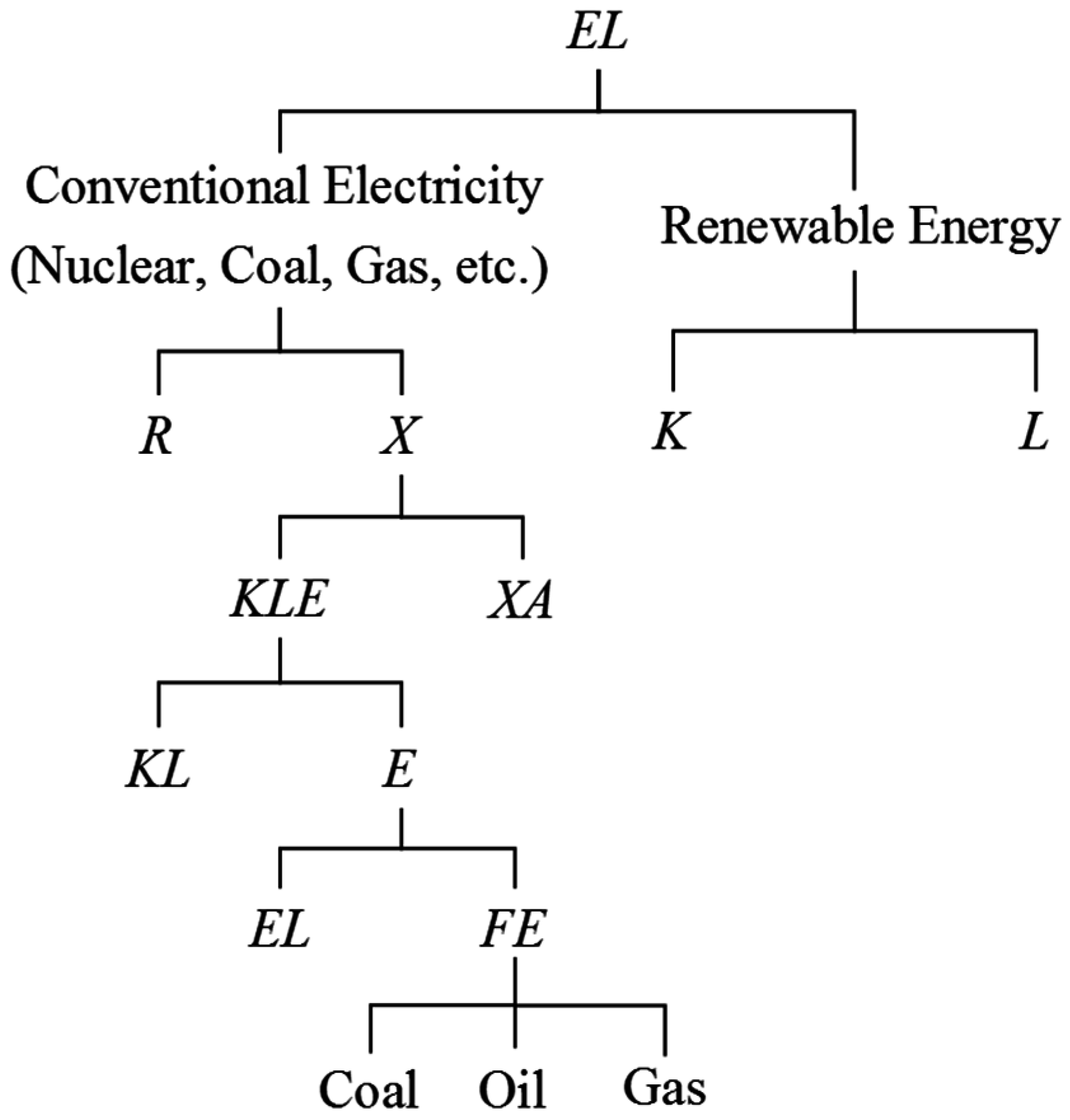
2.4.1. Electricity Industry

As mentioned in Section 2.1, it is difficult for the electricity supply to be jumped up in a short period of time to meet unexpected demand hikes. To encompass this feature, we introduce the upper-bound concept proposed by Bohringer and Rutherford [19]. Unlike commodities produced from factories, we assume the electricity sector has the fixed endowment of capital whose upper bounds are defined as the designed supply capacities. The reason to introduce the concept of the fixed endowment of capital is both to reflect the effects of electricity supply quantity due to the nuclear power phase out and to set up the constraint of electricity supply. The tree of the existing electricity generating technologies is shown in Figure 2.
The final electricity production and the fixed endowment of capital per each generating technology, Y e l e , t , is nested by the Leontief function to reflect the upper bound of each generating technology [20].
Y e l e , t = min [ X e l e , t ,   R e l e , t ]
R e l e , t is the composite electricity before being mixed with the fixed endowment of capital ( R ) and X e l e , t is the electricity constrained the fixed capacity ( X ). For the convenience of description, we do not use the subscript t representing the time.
We assume electricity market is the monopolistically competitive. The entry of rival firms leads to the equilibrium condition that the electricity bidding price of each generation technology is equal to the average cost.
P e l e = A C e l e
where the subscript e l e stands for each source generating electricity such as hydro, coal, gas, oil, nuclear and integrated power. P e l e and A C e l e indicates the price and average cost of e l e . Assuming the demand for an e l e is an inverse form of P ( X e l e ) , the monopolist’s revenue ( R V ) is as follows.
R V e l e = P ( Y e l e ) Y e l e
Accordingly, the Marginal revenue can be drown,
R V e l e Y e l e = P e l e + Y e l e P e l e X e l e = P e l e ( 1 1 ε e l e ) = P e l e ( 1 m k e l e )
where ε e l e is the Marshallian elasticity of demand, and m k e l e is the monopoly markup which is the inverse of the elasticity.
It is general that, under the condition of budget constraint, consumers try to maximize their utility by consuming nested electricity composited by CES function. We draw the demand function as follows,
Y e l e = P e l e σ ( P e l e 1 σ ) 1 M
where σ is the elasticity of substitution among electricity, and M is the household’s income.
Taking derivative and transforming the elasticity, we can ε e l e , the Marshallian elasticity of demand.
ε e l e = σ ( σ 1 ) s e l e
s e l e = P e l e Y e l e M = P e l e 1 σ ( P e l e 1 σ ) 1
where s e l e is the share of the income spent on e l e .
We can draw also electricity prices on the basis of the cost minimization approach.
P ( Y e l e ) = c ( P ( X e l e ) ,   P ( R e l e ) )
where P ( R e l e ) is the profit rate of the fixed capacity per each generating technology. c ( P ( X e l e ) ,   P ( R e l e ) ) is a marginal cost of generating one unit of Y e l e . Therefore, Equation (9) satisfies a zero profit condition.
Using the Shepard’s Lemma, we can draw a demand function of the fixed endowment of capital. We assume the supply of the fixed endowment of capital is given as estimated quantities and the revenue belongs to the household. Hence, Equation (10) of the supply and demand of the fixed capacity is determined as follows [21].
Y e l e c ( P ( X e l e ) ,   P ( R e l e ) ) P ( R e l e ) = R e l e ¯
where R e l e ¯ is the endowment of households on which the supply of electricity relies [19]. The equation means the electricity supply of the existing generating technologies cannot surpass the existing endowment which means R e l e ¯ is the upper bound of electricity supply from each generating technology. Hence, the phase-out of the nuclear power share causes reduction of the endowment which becomes the constraint of the supply from the nuclear power technology. This leads to raise an increase in the bidding price of the nuclear power, which influences the final electricity selling price in the end. In this research, we analyze the economic effects of the assumed share of nuclear phase-out by reflecting it into R e l e ¯ .
The electricity production of the existing generation technologies is assumed to follow CES function of labor-capital-energy composite goods and Armington goods [22]. The meaning of Armington goods is as follows. Consumption goods consist of commodities from not only domestically produced but also imported from other countries. Even though the goods exported are the same quality as those domestically produced, the price difference naturally brings about due to production costs and tariff. These characteristics incur incomplete substitution between goods domestically produced and imported from other countries. This phenomenon is defined as the Armington goods [23].
X e l e , t = [ α K L E e l e , t ρ + ( 1 α ) X A e l e , t ρ ] 1 ρ ,   ρ = σ 1 σ
Although distribution coefficient, ρ , should be different in every equation below, we express the same symbol for the simplicity. K L E e l e , t ρ is input composite factors of capital, labor and energy ( K L E ), and X A e l e , t ρ is Armington goods ( X A ).
We assumed that the production function of the existing electricity is nested by capital and labor and then input energy in turn as shown in Figure 2.
K L E e l e , i t = [ α K L e l e , i , t ρ + ( 1 α ) E e l e , i , t ρ ] 1 ρ
where K L e l e , i , t is the input factor of capital-labor to the existing electricity production i sector ( K L ) and E e l e , i , t is the input energy composite commodity in i sector ( E ).
Capital-labor composite is a CES function.
K L e l e , t = [ α K e l e , t ρ + ( 1 α ) L e l e , t ρ ] 1 ρ
where K and L are capital and labor respectively.
The energy production takes a CES function for electricity ( E L ) and non-electricity ( F E ) .
E e l e , t = [ α E L e l e , t ρ + ( 1 α ) F E e l e , t ρ ] 1 ρ
where F E is all energy sources excluding electricity which follows a CES function as well.
F E e l e , f e , t = f e [ α f e F E e l e , t ρ ] 1 ρ
In addition, we divide the conventional energy sources into coal, oil, gas to reflect the features of each generating technology.

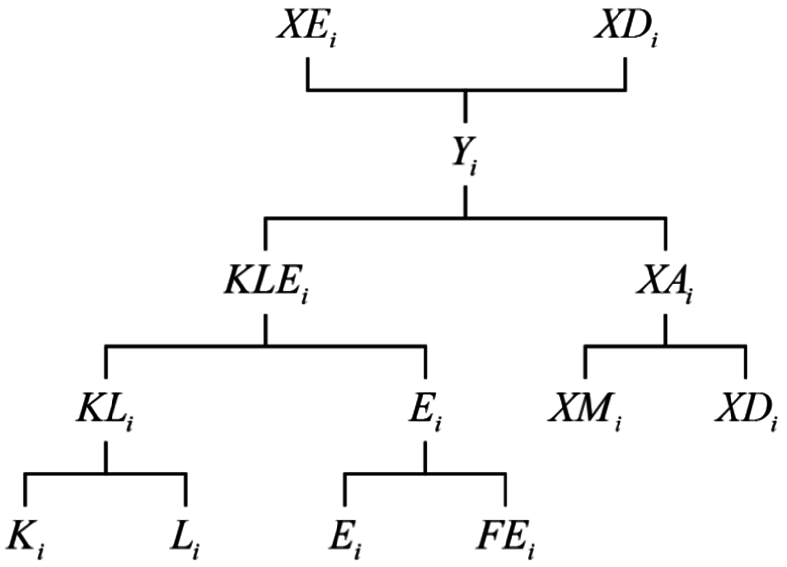
2.4.2. Non-Electricity Industry
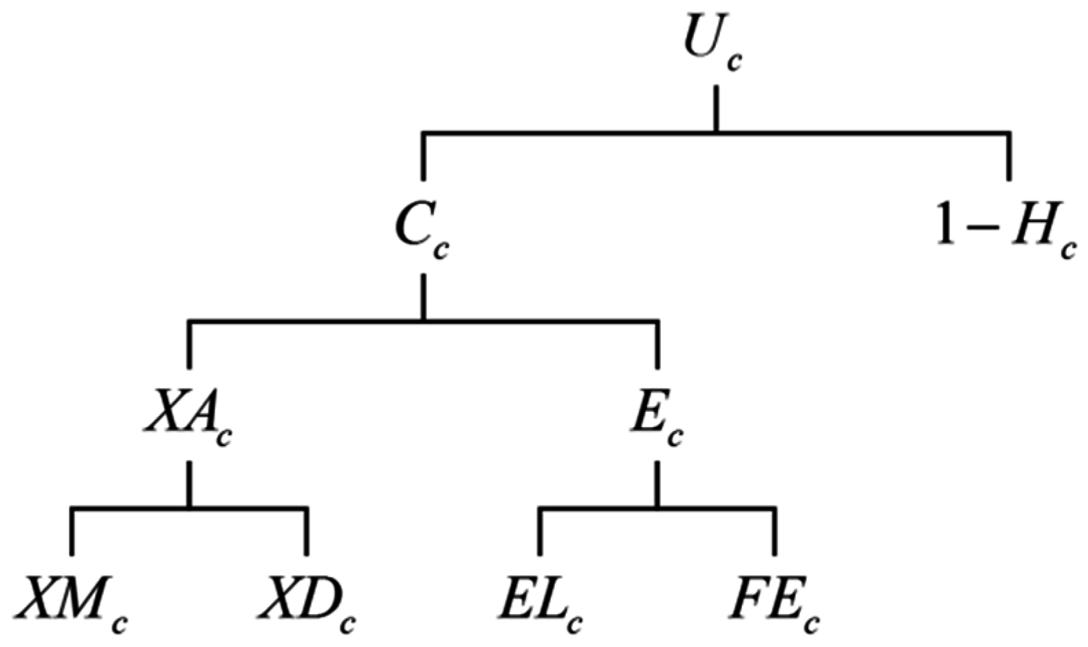
The final commodity of non-electricity industry is produced by the nested production phase (Figure 3). The production in the time period is a CES function of labor-capital-energy composite goods ( K L E i ) and Armington goods ( X A i ) . The final commodity produced in non-electricity industry is converted into export goods ( X E i ) and domestic goods ( X D i ) . Armington goods followed a CES function of the import goods ( X M i ) and domestic goods ( X D i ) in an incomplete substitution relation.

2.4.3. Household

Household is assumed as one representative. Its utility function ( U c ) is defined as follows.
max U ( C t , 1 H t ) = [ α C t ρ + ( 1 α ) L S t ρ ] 1 ρ
where C t is the consumption composite goods ( C c ) , L S t ρ is the leisure time ( 1 H c ) . The utility of household is established as in Figure 4.
The equation of income constraint is as follows. Each one is the after tax price.
p c , t C t + p k , t I k , t = ω t L t + r t K t + e l e p e l e , r , t R e l e , t + T r t
where p c , t is the price of consumption goods, p k , t is the price of investment, ω t is wage, r t is capital income, p e l e , r , t is the income of the fixed endowment of capital of the electricity sector. T r t is household income transferred from the government.
I t is the total investment which consists of the household and government savings and influx.
I t = S c , t + D g , t + B t
where S c , t is household savings, D g , t is government investment, B t is the influx of the balance of trade.
C t is consumption goods, which are nested between energy goods and non-energy goods.
C t = [ α X A c , n e , t ρ + ( 1 α ) E c , t ρ ] 1 ρ
where X A c , n e , t ρ is non-energy Armington goods consumed by household ( X A c ) . E c , t ρ is energy goods consumed by household ( E c ) .

2.4.4. Government

The government revenue is mostly from taxes which are spent on consuming and transferring to household.
Φ t + D g , t = i τ k , i , t R t K i , t + i τ l , i , t W t L i , t + i τ i , t P i , t Y i , t + i τ m , i , t R m , i , t X M i , t
where Φ t is the government total tax revenue and D g , t is government debt that is defined as its total revenue less total expenditure. R t and W t are wage rate and rate of return before tax respectively. τ k , i , t and τ l , i , t are an effective tax rate on corporate income and an average tax rate on labor income. P i , t is a price of i goods before tax. τ m , i , t is tariff rate. R m , i , t is a imported price before tax.
On the other hand, government expenditure ( Γ t ) is defined as follows.
Γ t = i p x a , i , t X A g , i , t + T g t
where p x a , i , t is after tax price of i Armington goods ( X A g , i , t ). T g t is government transfer to income groups.

2.4.5. International Trade

Assuming a small open economy, we regard the price of imported goods as exogenously given parameter. However, the imbalance of trade is settled by varying exchange rate.
i P x e , i , t X E i , t i P x m , i , t X M i , t + P e x , t B 0 = 0
where P x e , i , t and P x m , i , t are after tax prices of export and imported goods respectively. P e x , t is an exchange rate and B 0 is trade imbalance in the benchmark year. Hence, changing of P e x , t every year preserves the trade balance.

3. Input Data

3.1. Social Accounting Matrix (SAM)

SAM is a representation of the macro and micro economic accounts of a socio-economic system including the transactions and transfers among all economic agents. More technically, SAM is a square matrix in which each account is represented by a row and a column. Each cell shows the payment from the account of its column to the account of its row: the income of an account appear along its row, its expenditure along its column. Like other economic accounting systems, it captures transactions undertaken during a fiscal period, usually one year [24,25]. SAM provides the statistical basis of CGE model.
On the basis of the national account such as the 2010 Input-Output (IO) table and Statistical Yearbook of National Tax, Financial Statement Analysis and previous studies, we create the Social Accounting Matrix (SAM) considering features of the bottom-up electric characteristics and the unique Korean electricity industry to keep coherence between its micro data and those of IO table. The structure of the intermediate goods sold to the domestic industry is the 40-by-40 matrix (refer to Table 2), which is reduced from the 403-by-403 intermediate goods matrix.

3.1.1. Input-Output Table of the Electricity Industry

We divide electricity generating technologies into specific sectors type of fuels. Accordingly we assume the upper limit of each generating facility is the same as the estimated capacity designed when it was originally constructed. At the same time, we define the cross-subsidy as a mark-up which is the gap between the marginal cost and the selling price existed among generating facilities. In order to reasonably consider these features, we try to keep the consistency between macro data referred from input-output table and specific data from the electricity sector. We adjust the input-output table as follows. The conventional electricity sector of the input-output table consists of hydro, fossil, nuclear and other generating sources. Furthermore, we include independent power plants generated by diesel fuel into the fossil generating source and subdivide the fossil power into coal power, 51.9%, gas power, 39.4% and oil, 8.7% considering the 2010 selling ratio of fossil fuel generating technologies. In addition, as shown in Table 3, we adjust input fuels to reflect the features of the fossil fuel generating. For instance, all coal and its goods produced by coal, gas and its goods produced by gas and oil and its goods produced by oil are transferred to coal, gas and oil generating respectively.
Due to the fact that the 2010 input-output table does not provide the information of renewable energy, the output produced by each renewable source is estimated on the basis of the ratio of 2012 production. Especially, if we assume input factors for the production of electricity from renewable energy are labor and capital only. Thus, as demonstrated in Table 4, we classify the cost of labor and capital for the construction of the renewable energy inferred from the total value added of the electricity sector.
The output indicated in the IO table means revenue of each generating source. Accordingly the difference could often occur between the estimated ratio of each generating source in the IO table and that of the real output ratio of each. Hence, in this research, we define this difference as the cross-subsidy. As seen in the Table 5, the ratio of hydro, coal, gas, oil, nuclear and integrated energy is 1.1%, 33.3%, 25.3%, 5.6%, 27.3% and 7.4% respectively. Therefore, we adjust the ratio consistent with the real data which is the reference inferred from Sixth Electricity Supply and Demand Plan.
Table 6 indicates the revenue from electricity selling and the consumption ratio of electricity of each industrial sector respectively. Industrial sectors occupying higher ratio of electricity consumption are in the following order, the industries of wood and paper, other manufacturer, coal, metal, wholesale and retail, and leather (refer to Table 7). The household consumption of electricity is just 1.56% but contributing to the selling revenue is 20.9%.

3.1.2. Parameters and Calibration

As the modeling is finished, exogenous parameters are determined using the calibration process on the basis of SAM data made for this research. For instance, we calculate parameters of CES function used in this research by the following equation.
Y = E [ i = 1 n δ i X i ρ ] 1 ρ ,   ρ = σ 1 σ
where Y and X i ρ are output, and input factors each. A parameter needed to be calculated are efficient coefficient, E , and distribution coefficient, δ . Assuming elasticity of substitution, σ , and price of goods can be inferred from the IO table, distribution and efficient coefficient are able to be determined by the Equations (24) and (25) respectively.
δ j = P j X j 1 σ i = 1 n P i X i 1 σ
A = Y [ i = 1 n α i X i ρ ] 1 ρ
Exogenous parameters such as an elasticity of substitution, σ , not determined by calibration process above can be inferred from research results performed by experts.
For this research, we use elasticity of substitution for CES functions as shown in Table 8. Elasticity of substitution for CES and CET functions for this research refer to the results of the previous researches. In the production area, we use CET of export and domestic goods and Arminton goods as 2.5 which is the median value suggested by Sohn and Shin [26]. The elasticity of substitution between non-electricity energy sources is assumed to be 0.5, and that between electricity and non-electricity energy 0.3, and that between capital and labor 1. The elasticity of substitution between production factors and intermediate commodities 0, that between non-electricity sources used in the household 0.25, that that between electricity and non-electricity energy 0.5. The elasticity of substitution between consumption composite and leisure is assumed 0.5 [27].
As the economy can proceed with impacts more smoothly in the long term than in the short term, the elasticity of substitution in the inter-electricity industry is assumed to be gradually increased from 0.25 in 2010 to 0.5 in 2035.

4. Empirical Results

4.1. Bench Mark Data

We set up a bench mark scenario with the period of 2012 to 2035 consistent with the existing plans. Firstly, electricity facilities are composed based on the Sixth Electricity Supply and Demand Plan from 2012 to 2027. However, as a specific capacity of each electricity source is not known, we have to estimate the unknown capacity. Hence we define unknown generating capacities by calculating increasing rates from the capacities in 2027, the last year of the Sixth Electricity Supply and Demand Plan. Figure 5 shows the specific estimated capacities of each electricity generating source.

4.2. Scenario: Reduction of Nuclear Capacities

In order to analyze the impact of nuclear phase-out against the reference scenario, we made up of 4 scenarios as demonstrated in Table 9.
In Scenario 1, all types of nuclear power facilities are permitted of 10-year life extension, which resulted in just 5 nuclear power facilities phased out. In Scenario 2, 13 nuclear facilities are phased out sequentially up to the year of 2035. In Scenario 3, we designed 29% nuclear capacity of the total peak capacity suggested by the second national energy plan, In Scenario 4, PHWRs are not permitted of life extension, 8 plants are under construction, 14 PWR would start construction from 2024 as a result of which the peak capacity in 2035 could be 34.4%.
Figure 6 suggests the phase out capacities per scenario comparative to the reference scenario. In Scenario 1, there is no phase out capacity until 2017, starting from 587 MW phase-out in 2018 continues increasingly to 1600 MW (1.59%) in 2035. In Scenario 2, 1266 MW is assumed to be phased out in 2014 and 9037 MW (18.83%) in 2035. We especially design Scenario 3 to meet the second energy plan, which 679 MW is phased out in 2014, 10,500 MW (12.09%) in 2035 continuously. In Scenario 4, 679 MW is phased out in 2014 and then in 2027, 1379 MW phased out leads 2100 MW (4.85%) in 2035. To be noted, in all scenarios, the year 2031 suggests the largest reduction in capacity in order to satisfy each reduction plan compared with the reference case.

4.3. Analytical Results

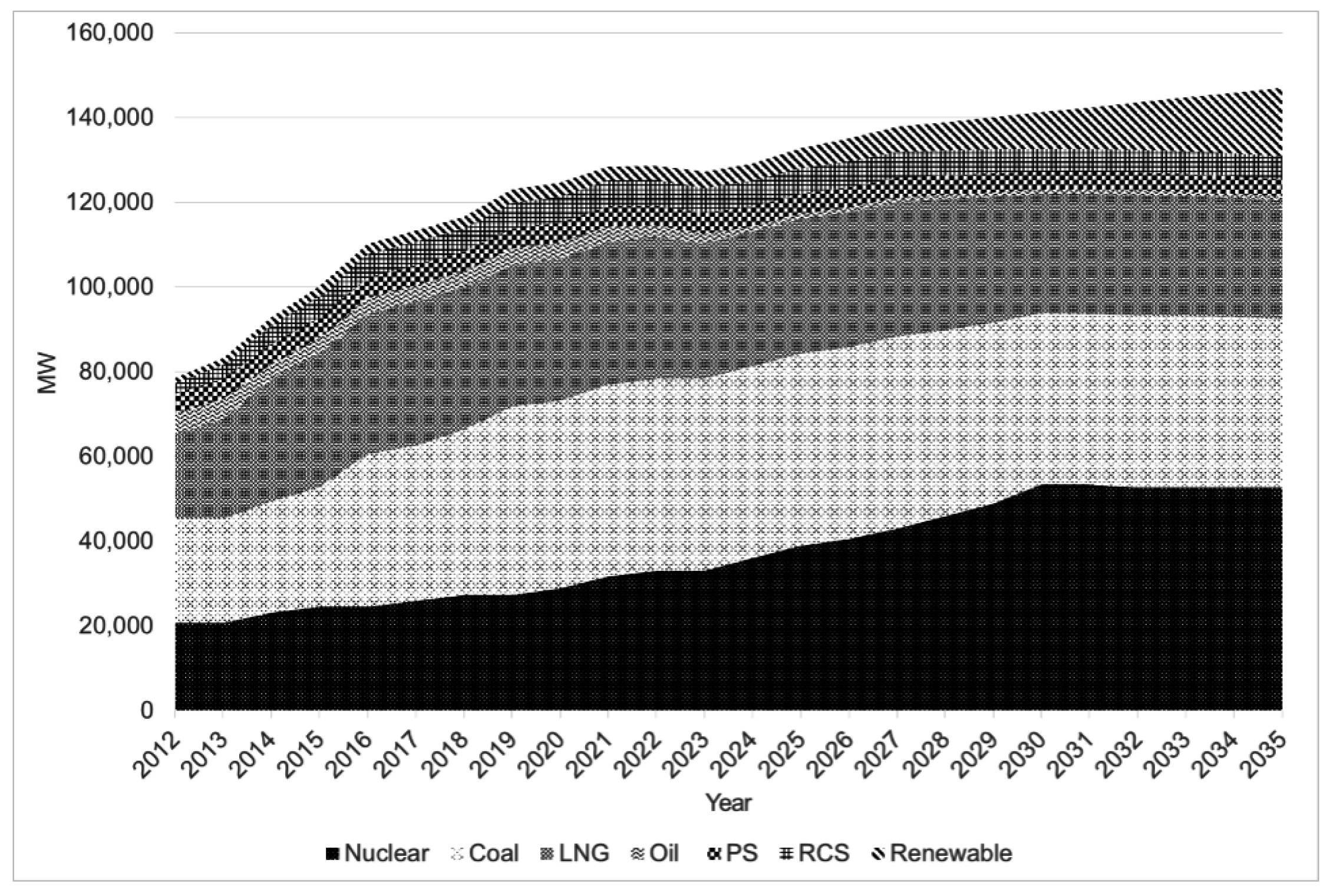
4.3.1. Electricity Industry

The reduction of nuclear power capacities, firstly, impacts the electricity industry itself. In this research, we analyze effects on the electricity selling price and electricity output per scenario. The changes of the electricity selling price of Scenario 2–4 respectively are shown in Figure 7. All Scenarios show the increase of the electricity selling prices. Especially, Scenario 2 and 3 demonstrate higher increases on average of 8.94% and 7.26% respectively. Scenario 3 represented as the second national energy plan shows the biggest increase of the electricity selling price from the year of 2024 and approached approximately a 15% increase. As the generation capacities from the nuclear power is not substituted by those of other generation technologies, it is anticipated that the reduction capacities of the nuclear power causes the decrease of overall electricity supply to eventually increase selling prices of electricity. Hence, the result of this research demonstrates the more phase out of the nuclear power, the higher the change of the electricity selling price.

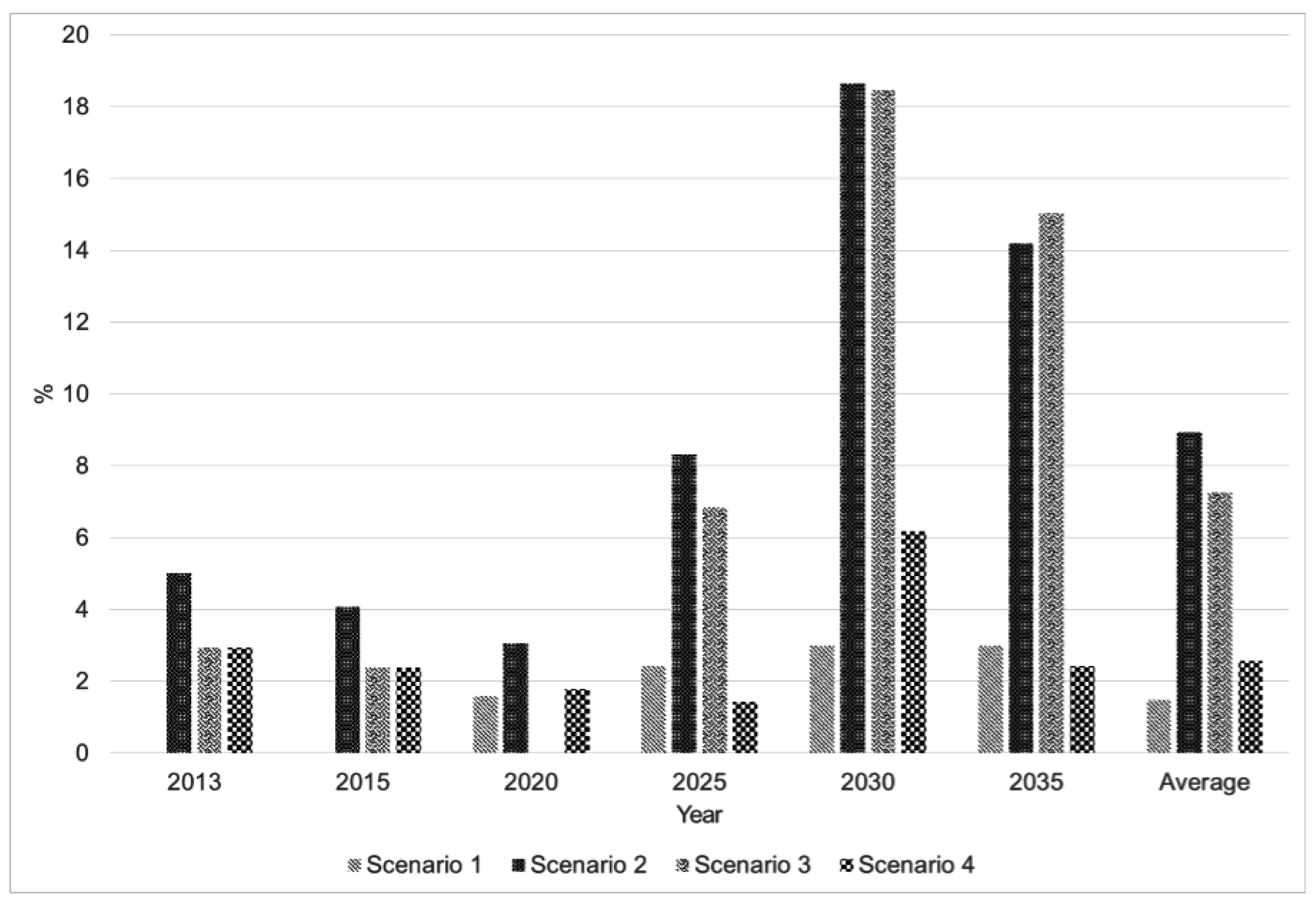
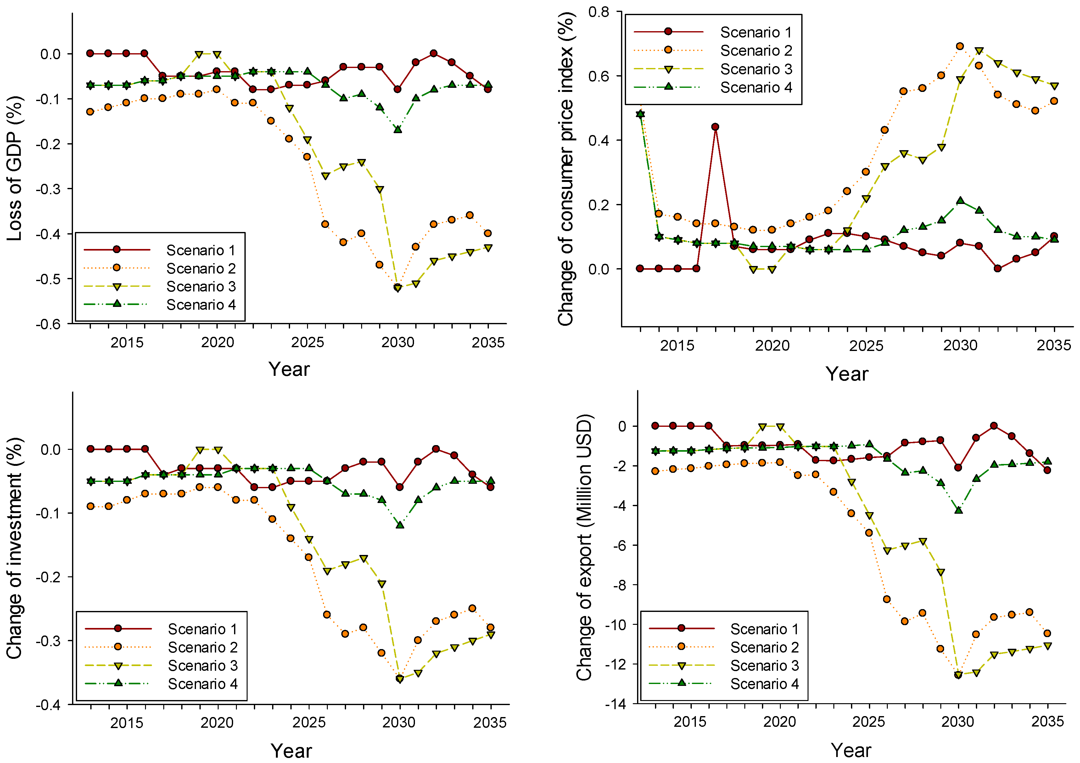
4.3.2. National Economic Effects

The reduction of the nuclear capacities influences not only the electricity industry but also national macro economy. In this section, we demonstrate the analysis results such as the reduction on GDP (Gross Domestic Gross), consumer price, consumption, investment, export, job market and the like Figure 8.
In case of GDP, Scenario 2 and 3 are influenced much higher than Scenario 1 and 4. The loss of GDP with comparison of the referenced scenarios is 0.08, 0.40, 0.43 and 0.07 with respect to Scenario 1–4. Compared to the reference, scenario 1 and 4 does not show any variations of reduction capacity in each year except the year of 2031. In addition, we can infer from the reduction capacity that the electricity production of scenario 1 and 4 outweighs that of scenario 2 and 3. Accordingly we reach the conclusion scenario 1 and 4 less influence on the domestic economy than scenario 2 and 3. Similarly the consumer prices are on the higher move with reduction of nuclear capacities. As shown in scenario 3, the consumer prices are increased 0.62%. However, the investment and export are decreased up to 0.29% and about 9.61 billion USD. It is the stereotype that the investment is determined by the substitution effects between the production scale and consumption variations. The reduction of the nuclear power directly impacts on the electricity selling price which causes the major trigger of the production reduction and in the end contributes to the investment curtail and vice versa. Figure 8 depicts the price increase of the consumer goods that has the direct relation to the consumption reduction.

4.3.3. Production Change of Industrial Sectors

The setback of the nuclear power supply gives a big influence on the domestic economy and each industry gets different impact depending on the electricity supply capacities. Table 10 shows production variations of the main industrial sectors. It is demonstrated that Industries such as chemical, steel, metal products heavily relied on the electric energy are severely impacted. The decreases in production of chemical, steel, metal products, cars and ships are 1.58%, 1.89%, 1.15%, 0.44% in 2035 respectively. Although the industries of electricity and electronics show small decrease compared with the industries above, the decrease of production is 0.07% in 2013 and 0.26% in 2035.

5. Conclusions and Policy Implications

As the recent catastrophic Fukushima accident throws a wet blanket over the world nuclear industry, many countries with currently operating nuclear power plants wonder about its safety and economic factors. Hence, we investigate the economic effects according to four reduction scenarios of nuclear power share in Korea. To capture those quantitative consequences, we use a hybrid CGE model with a detailed representation of the Korean electricity sector to well consider its bottom-up characteristics. In general, our research results show not only the electricity fare but also the macroeconomic index become worse as nuclear power capacities are in reduction. In specific, we find that Scenario 1 and 4, a minor reduction of nuclear power, until 2035 leads to moderate impacts on micro and macro economy. However, Scenario 2 and 3, which are the nuclear share targets of the Korean government, demonstrate the biggest magnitude of the negative impact on economy. Because the nuclear power facilities in Korea play a crucial role in energy sources, until innovative energy sources with good economics and efficiency are developed, it is necessary to keep the stable nuclear share for the Korean economy.
Our research shows the consistency per each scenario according to the reduction of the nuclear power share. Hence, our model could be extended in various respects. We, however, use the data estimated from the energy plan issued in 2008 rather than the new one formulated by the government. Hence, we need to simulate again when the new data reflecting recent economic index is issued. For further research, we plan to study and simulate the effects of the greenhouse gas emission in relation to the electricity industry.

Author Contributions

Taesik Yun: Developed the model and performed the experiments. Gyeong Lyeob Cho: He wrote the experimental section of the paper. Jang-yeop Kim: Created the overall idea and the basic outline of the paper.

Conflicts of Interest

The authors declare no conflict of interest.

References

  1. International Energy Agency (IEA). World Energy Outlook 2013; IEA: Paris, France, 2013. [Google Scholar]
  2. International Energy Agency (IEA). Energy Balances of OECD Countries; IEA: Paris, France, 2015. [Google Scholar]
  3. Bohringer, C.; Rutherford, T.F. Integrated assessment of energy policies: Decomposing top-down and bottom-up. J. Econ. Dyn. Control 2009, 33, 1648–1661. [Google Scholar] [CrossRef]
  4. Johansen, L. A Multi-Sectoral Study of Economic Growth; North-Holland: Amsterdam, The Netherlands, 1960. [Google Scholar]
  5. Harberger, A.C. The Incidence of the Corporation Income Tax. J. Political Econ. 1962, 70, 215–240. [Google Scholar] [CrossRef]
  6. Harberger, A.C. Efficiency Effects of Taxes on Income from Capital. In Effects of Corporation Income Tax; Krzyzaniak, M., Ed.; Wayne State University Press: Detroit, MI, USA, 1966; pp. 107–117. [Google Scholar]
  7. Scarf, H. On the Computation of Equilibrium Prices. In Ten Economic Studies in the Tradition from Irving Fischer; Fellner, W.J., Ed.; Wiley Press: New York, NY, USA, 1967. [Google Scholar]
  8. Scarf, H. The Computation of Economic Equilibria; Yale University Press: New Haven, CT, USA; London, UK, 1973. [Google Scholar]
  9. Fullerton, D.; Rogers, D.L. Who Bears the Lifetime Tax Burden? The Brooking Institution: Washington, DC, USA, 1993. [Google Scholar]
  10. Lau, A.P.; Rutherford, T.F. Approximation Infinite Horizon Models in a Complementarity Format: A Primer in Dynamic General Equilibrium Analysis. J. Econ. Dyn. Control 2002, 26, 577–609. [Google Scholar] [CrossRef]
  11. Uwe, R. Capacity Building through Energy Modelling and System Analysis; IEA: Paris, France, 2012. [Google Scholar]
  12. Hoffman, K.; Jorgenson, D. Economic and technological models for evaluation of energy policy. Bell J. Econ. 1976, 8, 444–466. [Google Scholar] [CrossRef]
  13. Hogan, W.W.; Weyant, J.P. Combined energy models. In Advances in the Economics of Energy and Resources; Moroney, J.R., Ed.; Emerald Group Publishing Limited: Bingley, UK, 1982; pp. 117–150. [Google Scholar]
  14. Drouet, L.; Haurie, A.; Labriet, M.; Thalmann, P.; Vielle, M.; Viguier, L. A Coupled Bottom-Up/Top-Down Model for GHG Abatement Scenarios in the Swiss Housing Sector; Energy and Environment; Springer: New York, NY, USA, 2005; pp. 27–61. [Google Scholar]
  15. Schäfer, A.; Jacoby, H. Experiments with a Hybrid CGE-MARKAL Model. Energy J. 2006, 27, 171–178. [Google Scholar] [CrossRef]
  16. Bahn, O.; Kypreos, S.; Bueller, B.; Luethi, H.J. Modelling an international market of CO2 emission permits. Int. J. Glob. Energy Issues 1999, 12, 283–291. [Google Scholar] [CrossRef]
  17. Messener, S.; Schrattenholzer, L. Message-Macro: Linking an energy supply model with a macroeconomic module and solving iteratively. Energy 2000, 25, 144–163. [Google Scholar] [CrossRef]
  18. Manne, A.S.; Mendelsohn, R.; Richels, R.G. MERGE: A model for evaluating regional and global effects of GHG reduction policies. Energy Policy 2006, 23, 17–34. [Google Scholar] [CrossRef]
  19. Boccanfuso, D.; Estache, A.; Savard, L. Electricity reforms in Mali: A macro-micro analysis of the effects on poverty and distribution. S. Afr. J. Econ. 2009, 77, 127–147. [Google Scholar] [CrossRef]
  20. Bosetti, V.; Carraro, C.; Galeotti, M.; Massetti, E.; Tavoni, M. WITCH—A World Induced Technical Change Hybrid Model; University Ca’Foscari of Venice Economic Research Paper, No.46/06; Social Science Electronic Publishing, Inc.: London, UK, 2006. [Google Scholar]
  21. Varian, H.R. Microeconomic Analysis, 3rd ed.; Norton: New York, NY, USA, 1992. [Google Scholar]
  22. Kim, M.K.; Kim, S.T. An Analysis on the Economic Effect of Corporate Income Tax Reduction in Korea Using Dynamic Computable General Equilibrium Model. Korean Econ. Rev. 2010, 58, 75–119. [Google Scholar]
  23. Armington, P.S. A theory of demand for products distinguished by place of production. IMF Staff Pap. 1969, 16, 159–178. [Google Scholar] [CrossRef]
  24. Pyatt, G.; Round, J.I. Social Accounting Matrix: A Basis for Planning; The World Bank: Washington, DC, USA, 1985. [Google Scholar]
  25. Reinert, K.A.; Roland-Holst, D.W. Social Accounting Matrices, Applied Method for Trade Policy: A Handbook; Cambridge University Press: Cambridge, UK, 1997; pp. 94–121. [Google Scholar]
  26. Sohn, Y.H.; Shin, D.C. The Effects of a Change in Exchange Rate on the Energy Sector in Korea. Korean Econ. Res. 1997, 45, 123–139. [Google Scholar]
  27. Bernstein, P.M.; Montgomery, W.O.; Rutherford, T.F. Global Impacts of the Kyoto Agreement: Results from MS-MRT Model. Resour. Energy Econ. 1999, 219, 375–413. [Google Scholar] [CrossRef]
Figure 1. Outline of CGE modeling.
Sustainability 08 01048 g001
Figure 2. Production tree of electricity generating sectors.
Sustainability 08 01048 g002
Figure 3. Production tree of non-electricity generating sectors.
Sustainability 08 01048 g003
Figure 4. Production Tree of Household.
Sustainability 08 01048 g004
Figure 5. Estimated peak generating capacities (MW). * PS: Pumped-Storage power plant; Source: the sixth electricity supply and demand plan and the second national energy plan.
Sustainability 08 01048 g005
Figure 6. Reduction capacities of nuclear power per scenario (MW).
Sustainability 08 01048 g006
Figure 7. Changes of electricity selling price (%).
Sustainability 08 01048 g007
Figure 8. Changes of macroeconomics per Scenario.
Sustainability 08 01048 g008
Table 1. Electricity generating technologies and their capacities in 2013.
TechnologyProduction (MW)Share (%)
Hydro with Pumped Storage47005.65
Coal thermal24,53429.49
Gas thermal23,57428.33
Oil thermal47805.74
Nuclear20,71624.90
Steam and Water Supply33065.65
Wind6430.77
Solar5340.64
Fuel cell4180.50
Table 2. Scope of Industry.
Scope of Industry
S01 Agriculture forestry and fishingS21 Hydro power
S02 Anthracite and flaming Coal productS22 Coal thermal power
S03 Other oil Product including crude oilS23 Gas thermal power
S04 Heavy and light oil productsS24 Oil thermal power
S05 Gas productsS25 Nuclear power
S06 MiningS26 Steam and water supply
S07 Food and beverageS27 Construction
S08 Textile and leatherS28 Wholesale and retails
S09 WoodS29 Accommodation and food service
S10 Paper and printingS30 Transportation and storage
S11 Coal productsS31 Communications and broadcasting
S12 Chemical productsS32 Financial and insurance
S13 Non-metallic productsS33 Real estate
S14 Basic metal productsS34 Public administration and national defense
S15 Metal productsS35 Education and human health
S16 MachineryS36 Social services
S17 Electrical and electronic instrumentsS37 Others service
S18 Precision machineryS38 Wind power
S19 Automobile and ship buildingS39 Solar power
S20 Other manufacturing productsS40 Fuel cell power
Table 3. Production costs of conventional generating sources in 2010. (Unit: Million USD).
HydroCoalGasOilNuclearRCS *Renewable
Domestic goodsCoal0122100000
Oil300818452150
Gas009196004190
Electricity1616229111925610
Other goods89195235613535182110
Import goodsCoal059890004890
Oil000101681690
Gas0000000
Electricity0000000
Other goods11222401535480
Value addedLabour1310229872066230252
Capital15012533391293739550427
TaxIndirect tax25185811744572860
Labour tax10640187158180
Corporate tax23965120568840
Tariff028200000
Cross subsidyMark-up23−630321260−207−17840
Total output249913,04510,696254011,0151256679
* RCS: Regional Cogeneration System.
Table 4. Production costs of renewable energy generating sources in 2010. (Unit: Million USD).
SolarWindFuel Cell
Labor9710946
Capital16418577
Total Output261295123
Table 5. Cross-subsidy among electricity generating sources.
HydroCoalGasOilNuclearRCSRenewable
2010 IO (%)1.133.325.35.627.37.4-
Reference (%)631.325.66.126.431.6
Cross-subsidy (Million USD)23−630321260−207−1784-
Table 6. Electricity selling revenue.
ClassificationIndustryFinal ConsumerExport Total Selling
Revenue (Million USD)32,9948735041,729
%79.120.9--
Table 7. Electricity consumption ratio.
ClassificationElectricity (Million USD)Total Output (Million USD)Electricity Consumption/Total Output (%)
Agricultural and marine33048,0830.69
Coal52262.29
Petroleum72265,9281.1
Heavy and light oil80451,0401.58
LNG and LPG2425,3710.09
Mineral products6028802.09
Food products and beverages52485,9830.61
Textile and leather products99046,3442.14
Wood and paper products82325,3863.24
Printing and publishing6176300.8
Coal products14769472.12
Chemical products2842203,4431.4
Non-metallic mineral products58531,1341.88
Basic metal products3551154,5262.3
Metal products1644111,3501.48
General machinery471103,5480.45
Electrical and electronic2154309,4760.7
Precise instruments7116,1400.44
Transport equipment923207,2390.45
Other manufacturing products3512352.8
Construction314171,2200.18
Whole sale and retail trade2815145,3991.94
Restaurant and accommodation94372,9691.29
Transport and storage556105,9640.52
Telecom and broadcasting83153,9981.54
Financial and insurance796120,9110.66
Real estate3855250,3681.54
Public administration85386,6330.98
Education and health2890162,0881.78
Social and other service97972,2251.36
Others42253,7970.78
Households8735559,1371.56
Table 8. Parameters: Elasticity of substitution.
GoodsElasticity of Substitution [σ]
Export goods vs. Domestic goods 2.5
Armington goods vs. General goods2.5
Between non electricity energies0.25
Non electricity vs. electricity0.5
Inter-electricity industry0.25–0.5 (assuming increase with time)
Consumption vs. leisure0.8
Elasticity vs. VA and energy0.7
Intra-fossil fuel substitution in final demand0.5
Elasticity of substitution vs. oil and gas2.0
Table 9. Scenarios.
Table 9. Scenarios.
ClassificationDescription
Reference Scenariophase-out of 2-plants, 2 times life extension of 20 years (total 44 plants operation)
Keeping 41% peak capacity of nuclear facility on the basis of the first national energy plan
8-plants of 1400 MW under construction and one 1000 MW PHWR
14-plants of 1500 MW in planning from 2024
35.8% peak capacity in 2035
Scenario 1one time life extension for all nuclear facilities for 10 years, 5-plant phase-out
8-plants of 1400 MW under construction and one 1000 MW PHWR, 14-plants of 1500 MW in planning from 2024
34.1% peak capacity in 2035
Scenario 2no permission of life extension to all nuclear facilities (total 13-plant phase-out)
8-plants of 1400 MW under construction and one 1000 MW PHWR, 14-plants of 1500 MW in planning from 2024
29% peak capacity in 2035
Scenario 3meeting the second national energy plan(total 2-plant phase-out)
8-plants of 1400 MW under construction and one 1000 MW PHWR
7-plants of 1500 MW in planning from 2024
28.7% peak capacity in 2035
Scenario 4no permission of life extension to PHWR, two times life extension for PWR (total 5-plant phase-out)
8-plant under construction, 14-plants of 1500 MW in planning from 2024
34.4% peak capacity in 2035
Table 10. Production changes of the main industrial sectors.
Agriculture FisheryChemicalSteelMetalElectricity ElectronicsCar ShipConstructionFinance Insurance
2013−0.05−0.28−0.34−0.21−0.07−0.1−0.07−0.06
2014−0.04−0.27−0.33−0.2−0.07−0.09−0.07−0.06
2015−0.04−0.26−0.32−0.2−0.07−0.09−0.06−0.06
2016−0.04−0.24−0.29−0.18−0.06−0.08−0.06−0.05
2017−0.04−0.22−0.27−0.17−0.06−0.08−0.05−0.05
2018−0.03−0.21−0.25−0.16−0.05−0.07−0.05−0.05
201900000000
202000000000
2021−0.03−0.18−0.22−0.14−0.04−0.06−0.04−0.04
2022−0.03−0.18−0.21−0.13−0.04−0.06−0.04−0.04
2023−0.03−0.18−0.21−0.13−0.04−0.06−0.04−0.04
2024−0.08−0.47−0.57−0.35−0.11−0.15−0.11−0.1
2025−0.12−0.74−0.9−0.56−0.16−0.24−0.18−0.16
2026−0.17−1.02−1.23−0.76−0.22−0.32−0.25−0.22
2027−0.16−0.97−1.17−0.72−0.2−0.3−0.24−0.21
2028−0.15−0.92−1.1−0.68−0.18−0.28−0.23−0.2
2029−0.19−1.15−1.38−0.85−0.22−0.34−0.29−0.25
2030−0.33−1.94−2.33−1.43−0.36−0.57−0.49−0.42
2031−0.32−1.89−2.27−1.39−0.35−0.55−0.48−0.41
2032−0.29−1.72−2.07−1.26−0.31−0.49−0.44−0.37
2033−0.28−1.68−2.01−1.23−0.29−0.47−0.43−0.36
2034−0.28−1.63−1.95−1.19−0.28−0.46−0.41−0.35
2035−0.27−1.58−1.89−1.15−0.26−0.44−0.4−0.34

