
Demand Side Management Performance Evaluation for Commercial Enterprises

Abstract
:1. Introduction
- (1)
- To the best of our knowledge, this is the first study on DSM performance in the commercial sector. We provided a detailed and complete evaluation list of economic, social, environmental and technical criteria to evaluate the DSM effects.
- (2)
- The fuzzy AHP and the fuzzy TOPSIS methods have been employed in many research fields [28,29,30,31,32] and have good effects in decision-making procedures of alternatives evaluation. As we know, this is a hybrid MCDM model based on combining the fuzzy AHP weight method with the fuzzy TOPSIS approach. We have introduced the model into DSM performance evaluation and extended the application fields of these methods.
- (3)
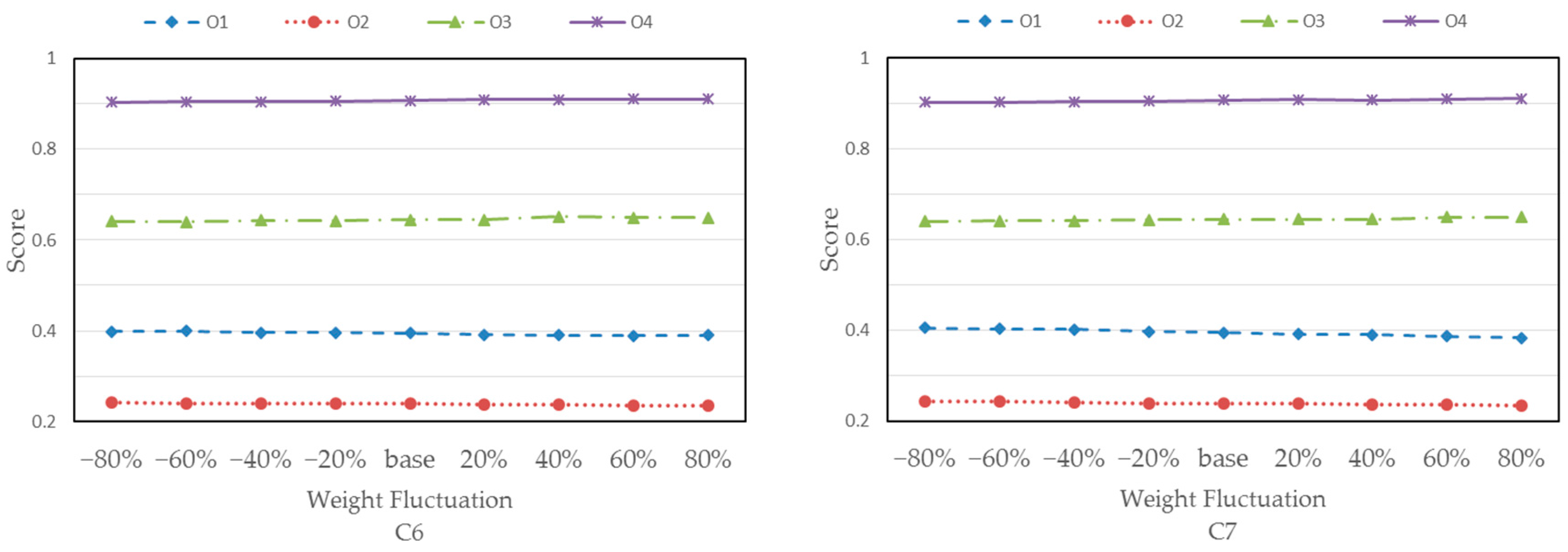
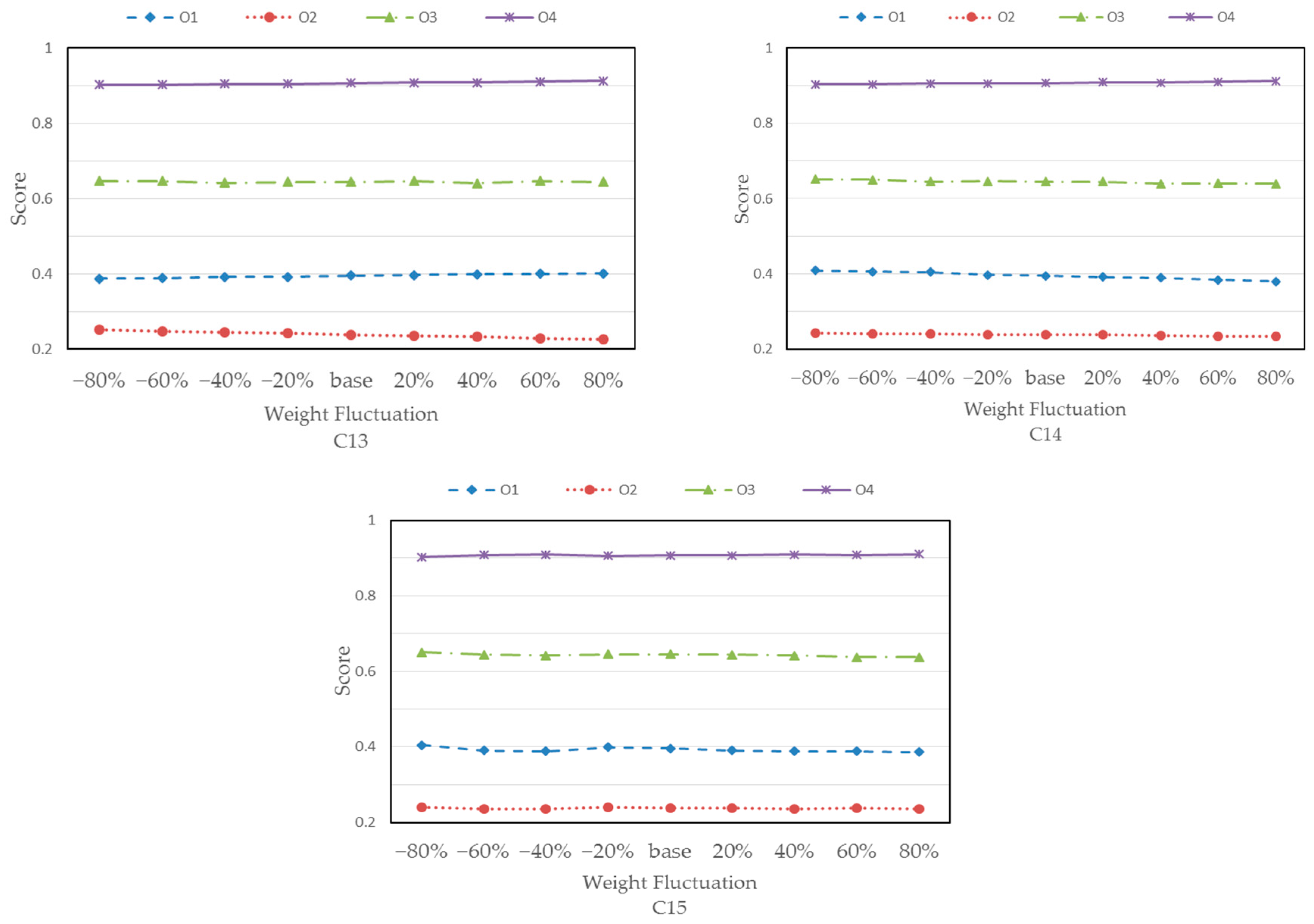
- Since experts with diverse professional backgrounds may give different decisions, it is necessary to probe the influences of sub-criteria weights on final decision-making. We gave a novel sensitivity analysis to research the performance of economic, social, environmental and technological criteria for DSM performance evaluation by modifying the sub-criteria weights.
2. Methods
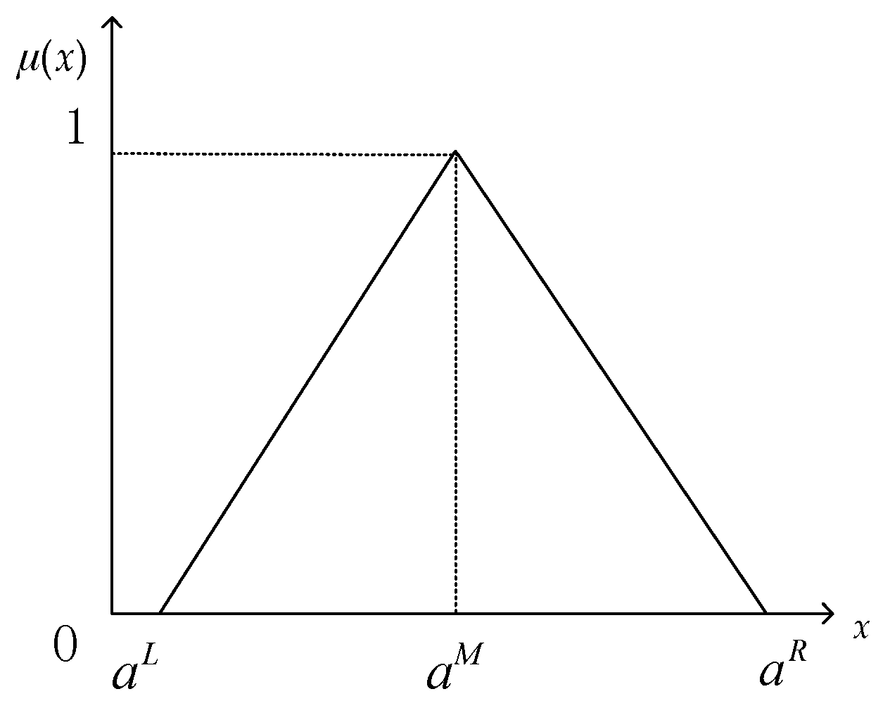
2.1. Fuzzy Set Theory and Fuzzy Numbers
2.2. Fuzzy AHP Weighting Method
2.3. Fuzzy TOPSIS Method
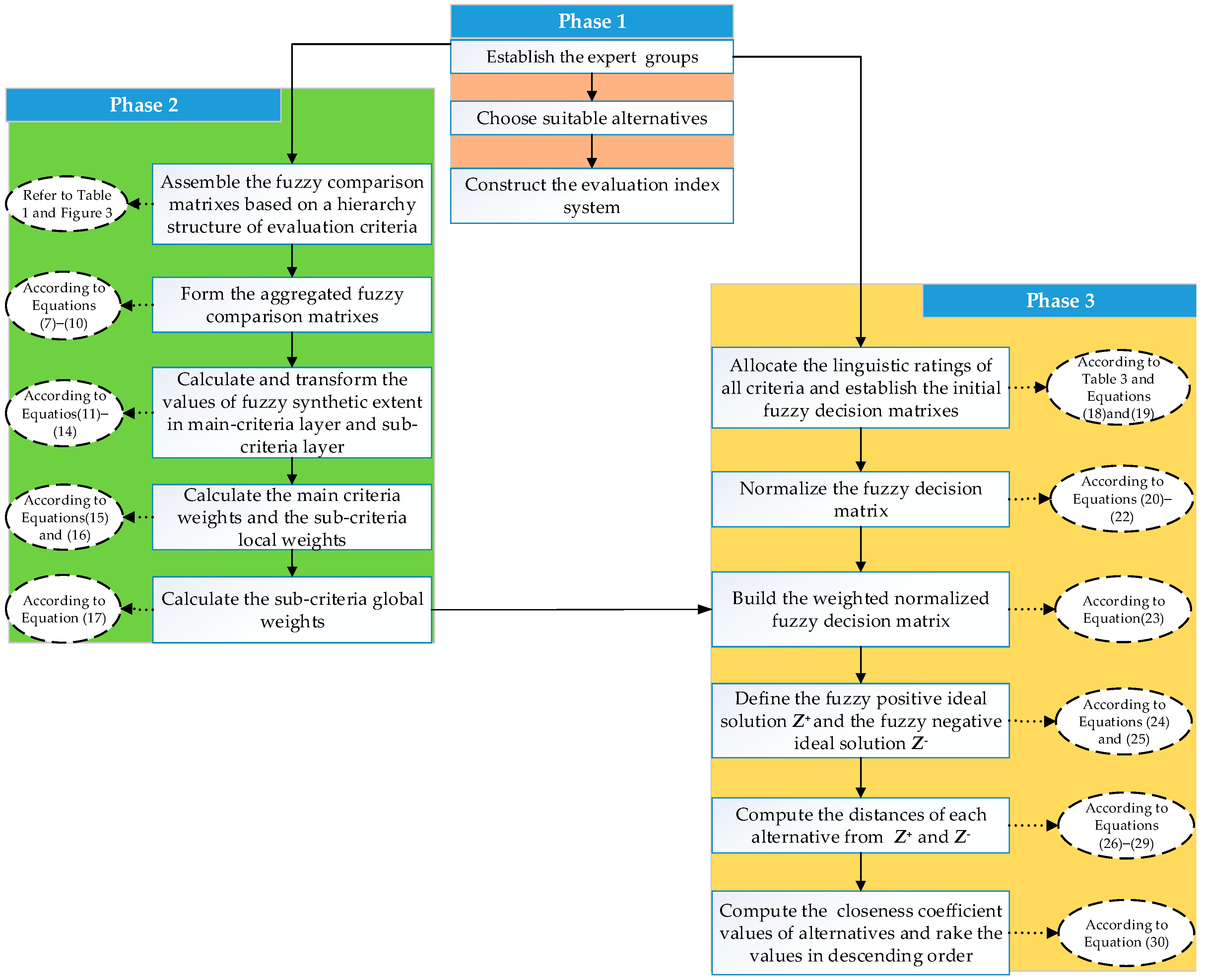
2.4. The Framework of Proposed Hybrid Fuzzy AHP-TOPSIS Model
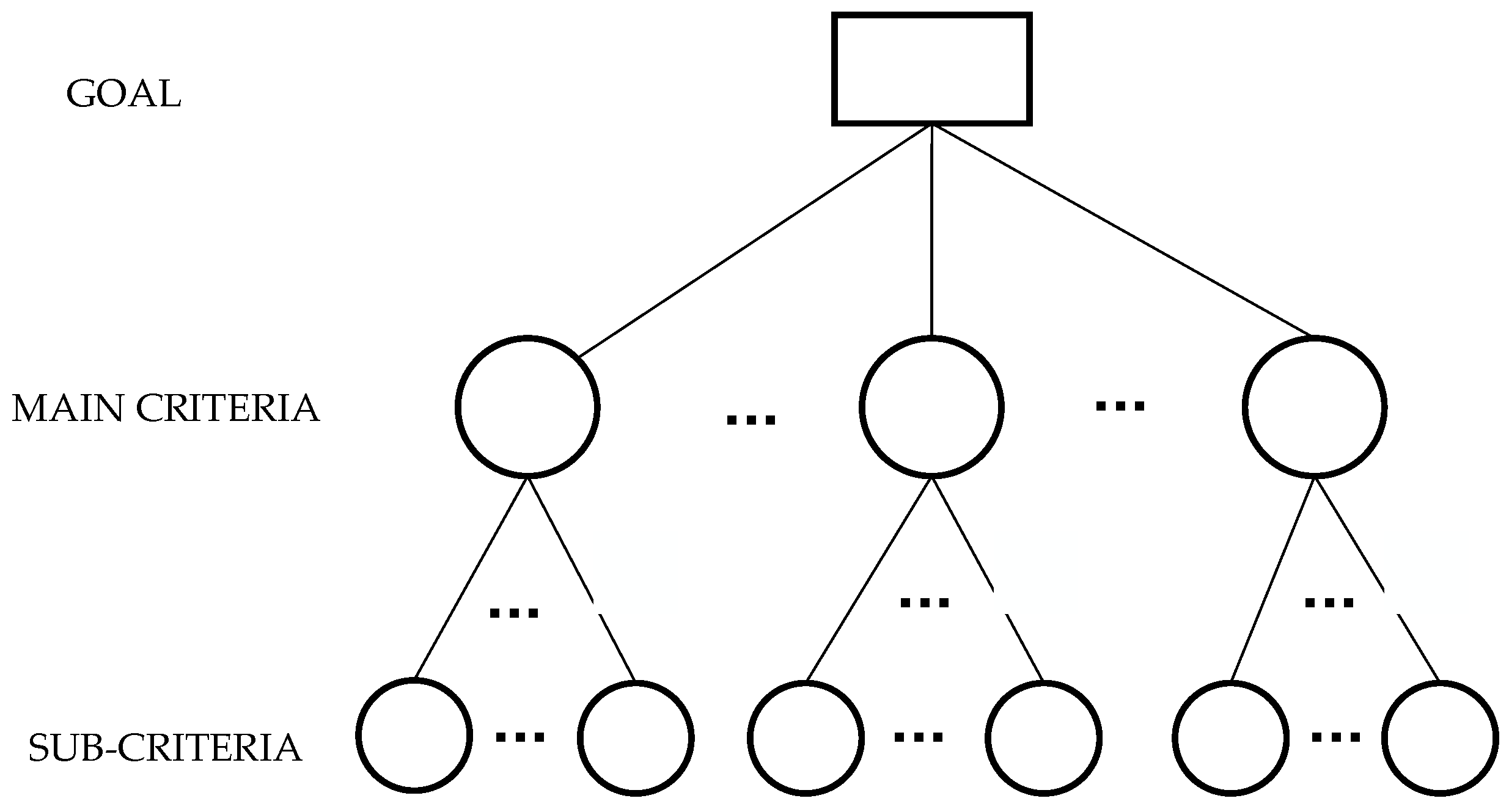
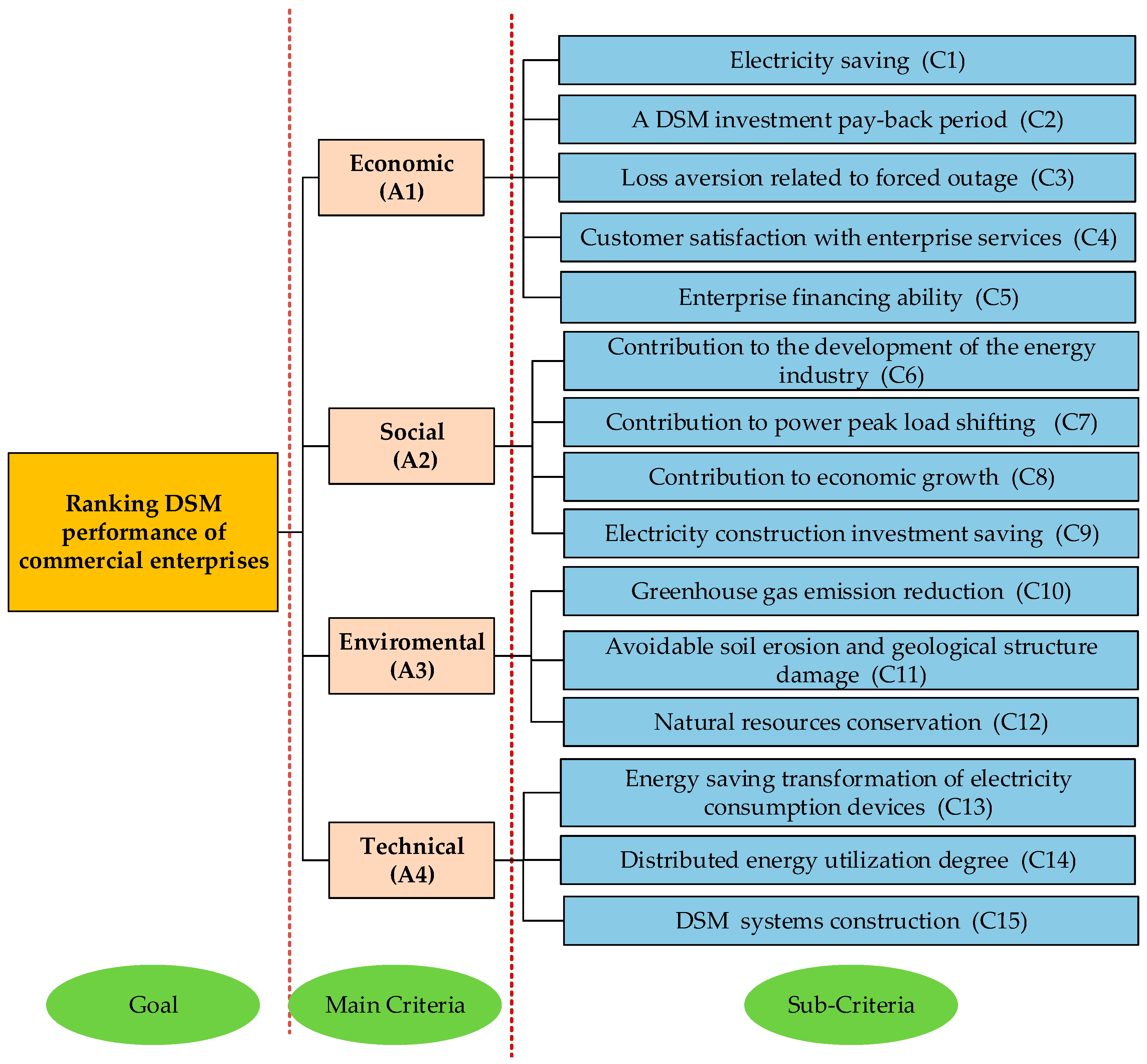
3. Evaluation Index System for the DSM Performance of Commercial Enterprises
3.1. Economic Criteria (A1)
- (1)
- Electricity savings (C1): Measure the reduction of the electricity consumption per unit area by implementing DSM. Appropriate energy efficient programs can help the enterprises achieve their goals to save energy.
- (2)
- A DSM investment pay-back period (C2): Refers to total investment cost of DSM divided by monthly returns. This sub-criterion measures the economic benefit for enterprises.
- (3)
- Loss aversion related to forced outage (C3): Refers to losses from service interruptions caused by forced outage. The forced outage probability can be reduced if an enterprise participates in DSM.
- (4)
- Customer satisfaction with enterprise services (C4): Measures the impacts on customers’ subjective enjoyment for the services provided under DSM implementation. For the commercial sector, higher customer satisfaction brings more business profits.
- (5)
- Enterprise financing ability (C5): Refers to financing channels and fundraising scales faced by these enterprises. A lot of capital investment is required for DSM implementation.
3.2. Social Criteria (A2)
- (1)
- Contribution to the development of the energy industry (C6): includes the energy saving service corporations, the distributed micro-grid systems etc.
- (2)
- Contribution to power peak load shifting (C7): helps increase penetration of the renewable energy sources and improve operation reliability of the power grid.
- (3)
- Contribution to economic growth (C8): Refers to the contribution degree of the DSM implementations to ensure energy supply security and maintain sustainable economic development.
- (4)
- Electricity construction investment saving (C9): Measures avoidable power generation equipment investment due to the electricity consumption reduction and avoidable power grid investment due to the load transfer.
3.3. Environmental Criteria (A3)
- (1)
- Greenhouse gas emission reduction (C10): Measures the reduction of the environmental pollutant (such as CO2 and NO2) emissions from the power generation sector due to DSM.
- (2)
- Avoidable soil erosion and geological structure damage (C11): Measures the reduction of occurrence probability for soil erosion and geological structure damage benefiting from DSM.
- (3)
- Natural resources conservation (C12): DSM is conducive to cutting the energy demand, which is good to save limited natural resources, especially fossil fuel [3]. This sub-criterion measures the reduction of the natural resources consumption by cutting the energy demand because of DSM.
3.4. Technical Criteria (A4)
- (1)
- Energy saving transformation of electricity consumption devices (C13): Measures the applications of energy saving equipment and technologies in a power system, including lighting, air conditioning and heating. The sub-criterion reflects energy saving technological levels of enterprises.
- (2)
- Distributed energy utilization degree (C14): Refers to the application of a distributed energy technology into a cooling-heating-power combined cycle, which helps to improve the energy resources comprehensive utilization efficiency of the energy resources and the continuity and reliability of energy supply. The distributed power generation technology, the smart micro grid technology and the distributed energy storage technology are basically adopted by entrepreneurs [43].
- (3)
- DSM systems construction (C15): Includes appointing directors, hiring full-time management personnel and training technical staff, which are based on enterprise status in order to ensure the effectiveness and continuity of DSM implementation.
4. Empirical Analysis
4.1. Determine the Weights of All the Criteria based on the Fuzzy AHP Technique
4.2. Assemble the Initial Fuzzy Decision Matrix
4.3. Calculate the Fuzzy Positive Ideal Solution and the Fuzzy Negative Ideal Solution
4.4. Determine the Preference Rakings of the Alternatives
5. Discussion
6. Conclusions
- (1)
- It is found that C10 and C12 affiliated with the environment criteria obtain more attention from experts, and alternative O4 was chosen as the best, followed by O3, O1 and O2;
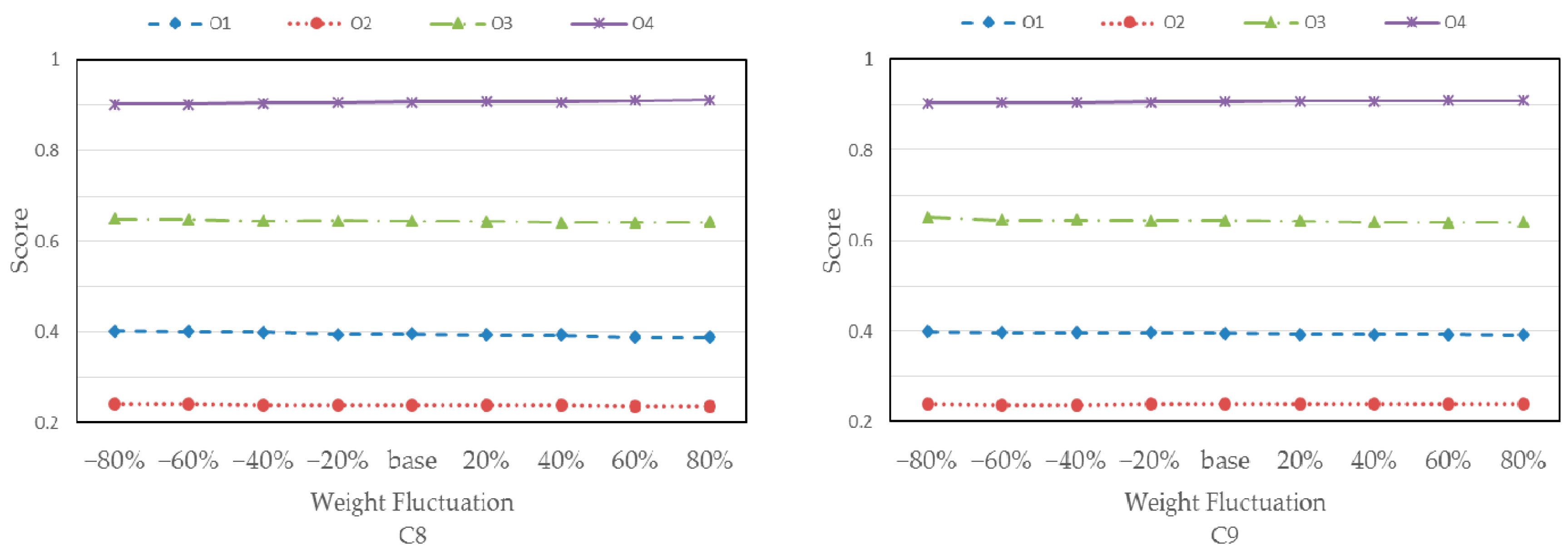
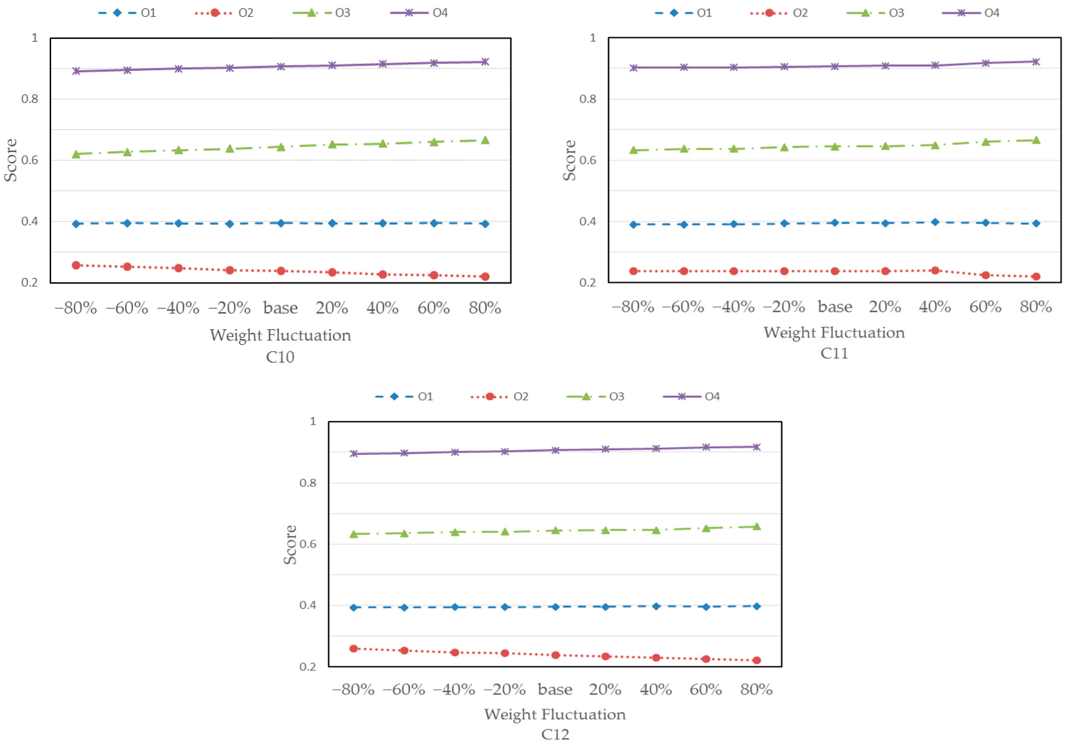
- (2)
- A sensitivity analysis for the sub-criteria weights were performed to test the robustness and effectiveness of evaluation results, which indicated that the ranking results remain stable no matter how the weights of the sub-criteria change.
Acknowledgments
Author Contributions
Conflicts of Interest
References
- Zhao, H.; Guo, S.; Fu, L. Review on the costs and benefits of renewable energy power subsidy in China. Renew. Sustain. Energy Rev. 2014, 37, 538–549. [Google Scholar] [CrossRef]
- Wang, H.; Zhang, Y.; Lu, X.; Nielsen, C.P.; Bi, J. Understanding China’s carbon dioxide emissions from both production and consumption perspectives. Renew. Sustain. Energy Rev. 2015, 52, 189–200. [Google Scholar] [CrossRef]
- Zhou, K.; Yang, S. Demand side management in China: The context of China’s power industry reform. Renew. Sustain. Energy Rev. 2015, 52, 954–965. [Google Scholar] [CrossRef]
- Ming, Z.; Song, X.; Mingjuan, M.; Lingyun, L.; Min, C.; Yuejin, W. Historical review of demand side management in China: Management content, operation mode, results assessment and relative incentives. Renew. Sustain. Energy Rev. 2015, 25, 470–482. [Google Scholar] [CrossRef]
- Strbac, G. Demand side management: Benefits and challenges. Energy Policy 2008, 36, 4419–4426. [Google Scholar] [CrossRef]
- Zeng, M.; Yang, Y.; Wang, L.; Sun, J. The power industry reform in China 2015: Policies, evaluations and solutions. Renew. Sustain. Energy Rev. 2016, 57, 94–110. [Google Scholar] [CrossRef]
- Zhang, X.P.; Cheng, X.M. Energy consumption, carbon emissions, and economic growth in China. Ecol. Econ. 2009, 68, 2706–2712. [Google Scholar] [CrossRef]
- Zhao, Z.; Yu, C.; Yew, M.; Liu, M. Demand side management: A green way to power Beijing. J. Renew. Sustain. Energy 2015, 7, 041505. [Google Scholar] [CrossRef]
- Arteconi, A.; Hewitt, N.J.; Polonara, F. State of the art of thermal storage for demand-side management. Appl. Energy 2012, 93, 371–389. [Google Scholar] [CrossRef]
- Eissa, M.M. Demand side management program evaluation based on industrial and commercial field data. Energy Policy 2011, 39, 5961–5969. [Google Scholar] [CrossRef]
- Albadi, M.H.; Saadany, E.F. A summary of demand response in electricity markets. Electr. Power Syst. Res. 2008, 78, 1989–1996. [Google Scholar] [CrossRef]
- Wang, J.; Bloyd, C.N.; Hu, Z.; Tan, Z. Demand response in China. Energy 2010, 35, 1592–1597. [Google Scholar] [CrossRef]
- Cobuloglu, H.I.; Büyüktahtakın, İ.E. A stochastic multi-criteria decision analysis for sustainable biomass crop selection. Exp. Syst. Appl. 2015, 42, 6065–6074. [Google Scholar] [CrossRef]
- Papaefthymiou, G.; Hasche, B.; Nabe, C. Potential of heat pumps for demand side management and wind power integration in the German electricity market. IEEE Trans. Sustain. Energy 2012, 3, 636–642. [Google Scholar] [CrossRef]
- Lund, H.; Kempton, W. Integration of renewable energy into the transport and electricity sectors through V2G. Energy Policy 2008, 36, 3578–3587. [Google Scholar] [CrossRef]
- Sianaki, O.A.; Hussain, O.; Dillon, T.; Tabesh, A.R. Intelligent decision support system for including consumers’ preferences in residential energy consumption in smart grid. In Proceedings of the Second International Conference on Computational Intelligence, Modelling and Simulation, Liverpool, UK, 28–30 September 2010.
- Tanoto, Y.; Santoso, M.; Hosea, E. Multi-dimensional assessment for residential lighting demand side management: A proposed framework. Appl. Mech. Mater. 2013, 284, 3612–3616. [Google Scholar] [CrossRef]
- Miara, A.; Tarr, C.; Spellman, R.; Vörösmarty, C.J.; Macknick, J.E. The power of efficiency: Optimizing environmental and social benefits through demand-side-management. Energy 2014, 76, 502–512. [Google Scholar] [CrossRef]
- Dawadi, S, Ahmad, S. Evaluating the impact of demand-side management on water resources under changing climatic conditions and increasing population. J. Environ. Manag. 2013, 114, 261–275. [Google Scholar]
- Gudi, N.; Wang, L.; Devabhaktuni, V. A demand side management based simulation platform incorporating heuristic optimization for management of household appliances. J. Environ. Manag. 2012, 43, 185–193. [Google Scholar] [CrossRef]
- Pina, A.; Silva, C.; Ferrão, P. The impact of demand side management strategies in the penetration of renewable electricity. Energy 2012, 41, 128–137. [Google Scholar] [CrossRef]
- Fehrenbach, D.; Merkel, E.; McKenna, R.; Karl, U.; Fichtner, W. On the economic potential for electric load management in the German residential heating sector—An optimizing energy system model approach. Energy 2014, 71, 263–276. [Google Scholar] [CrossRef]
- Dallinger, D.; Wietschel, M. Grid integration of intermittent renewable energy sources using price-responsive plug-in electric vehicles. Renew. Sustain. Energy Rev. 2012, 16, 3370–3382. [Google Scholar] [CrossRef]
- Lee, D.K.; Park, S.Y.; Park, S.U. Development of assessment model for demand-side management investment programs in Korea. Energy Policy 2007, 35, 5585–5590. [Google Scholar] [CrossRef]
- Aalami, H.A.; Moghaddam, M.P.; Yousefi, G.R. Modeling and prioritizing demand response programs in power markets. Electr. Power Syst. Res. 2010, 80, 426–435. [Google Scholar] [CrossRef]
- Yang, L.; Deuse, J. Multiple-attribute decision making for an energy efficient facility layout design. Procedia CIRP 2012, 3, 149–154. [Google Scholar] [CrossRef]
- Saaty, T.L. What is the analytic hierarchy process? Math. Model. Decis. Support 1988, 48, 109–121. [Google Scholar]
- Sianaki, O.A.; Masoum, M.A. A fuzzy TOPSIS approach for home energy management in smart grid with considering householders’ preferences. In Proceedings of the 2013 IEEE PES Innovative Smart Grid Technologies (ISGT), Washington, DC, USA, 24–27 February 2013.
- Ciabattoni, L.; Ferracuti, F.; Grisostomi, M.; Ippoliti, G.; Longhi, S. Fuzzy logic based economic analysis of photovoltaic energy management. Neurocomputing 2015, 170, 296–305. [Google Scholar] [CrossRef]
- Choudhary, D.; Shankar, R. An STEEP-fuzzy AHP-TOPSIS framework for evaluation and selection of thermal power plant location: A case study from India. Energy 2012, 42, 510–521. [Google Scholar] [CrossRef]
- Chang, D.Y. Applications of the extent analysis method on fuzzy AHP. Eur. J. Oper. Res. 1996, 95, 649–655. [Google Scholar] [CrossRef]
- Chen, C.T. Extensions of the TOPSIS for group decision-making under fuzzy environment. Fuzzy Sets Syst. 2000, 114, 1–9. [Google Scholar] [CrossRef]
- Zadeh, L.A. Fuzzy sets as a basis for a theory of possibility. Fuzzy Sets Syst. 1978, 1, 3–28. [Google Scholar] [CrossRef]
- Mardani, A.; Jusoh, A.; Zavadskas, E.K. Fuzzy multiple criteria decision-making techniques and applications—Two decades review from 1994 to 2014. Exp. Syst. Appl. 2015, 42, 4126–4148. [Google Scholar] [CrossRef]
- Liao, H.; Xu, Z.; Zeng, X.J. Distance and similarity measures for hesitant fuzzy linguistic term sets and their application in multi-criteria decision making. Inform. Sci. 2014, 271, 125–142. [Google Scholar] [CrossRef]
- Chen, S.H.; Li, G.C. Representation, ranking and distance of fuzzy number with exponential membership function using graded mean integration method. Tamsui Oxf. J. Manag. Sci. 2000, 16, 123–131. [Google Scholar]
- Zhao, H.; Guo, S. Selecting green supplier of thermal power equipment by using a hybrid MCDM method for sustainability. Sustainability 2014, 6, 217–235. [Google Scholar] [CrossRef]
- Gold, S.; Awasthi, A. Sustainable global supplier selection extended towards sustainability risks from (1 + n)th tier suppliers using fuzzy AHP based approach. IFAC-PapersOnLine 2015, 48, 966–971. [Google Scholar] [CrossRef]
- Li, H.; Guo, S. External economies evaluation of wind power engineering project based on analytic hierarchy process and matter-element extension model. Math. Probl. Eng. 2013, 2013. [Google Scholar] [CrossRef]
- Saaty, T.L. Decision making—The analytic hierarchy and network processes (AHP/ANP). J. Syst. Sci. Syst. Eng. 2004, 13, 1–35. [Google Scholar] [CrossRef]
- Junior, F.R.L.; Osiro, L.; Carpinetti, L.C.R. A comparison between Fuzzy AHP and Fuzzy TOPSIS methods to supplier selection. Appl. Soft Comput. 2014, 21, 194–209. [Google Scholar] [CrossRef]
- Li, D.F. Compromise ratio method for fuzzy multi-attribute group decision making. Appl. Soft Comput. 2007, 7, 807–817. [Google Scholar] [CrossRef]
- Wang, Y.; Wang, J.; Dong, X.; Du, P.; Ni, M.; Wang, C.; Yao, L.; Zhang, B. Guest Editorial Smart Grid Technologies and Development in China. IEEE T. Smart Grid 2016, 7, 379–380. [Google Scholar] [CrossRef]
- Li, M.; Zhang, L. Haze in China: Current and future challenges. Environ. Pollut. 2014, 189, 85–86. [Google Scholar] [CrossRef] [PubMed]
- Wang, T.; Yan, C.Z.; Song, X.; Li, S. Landsat images reveal trends in the aeolian desertification in a source area for sand and dust storms in China’s Alashan Plateau (1975–2007). Land Degrad. Dev. 2013, 24, 422–429. [Google Scholar] [CrossRef]
- Zweig, D.; Eriksen, S.S. China’s Energy Anxiety. In Sino-US Energy Triangles: Resource Diplomacy under Hegemony; Routledge: Abingdon, UK, 2015; p. 256. [Google Scholar]

 ’, ‘
’, ‘  ’, ‘
’, ‘  ’, ‘
’, ‘  ’, ‘
’, ‘  ’, ‘
’, ‘  ’, ‘
’, ‘  ’, ‘
’, ‘  ’, ‘
’, ‘  ’, ‘
’, ‘  ’, ‘
’, ‘  ’, ‘
’, ‘  ’, ‘
’, ‘  ’, ‘
’, ‘  ’, and ‘
  ’ represent the performance of C1, C2, C3, C4, C5, C6, C7, C8, C9, C10, C11, C12, C13, C14 and C15, respectively; (2) black, blue, red and green represent alternatives O1, O2, O3 and O4, respectively; and (3) X-axis, Y-axis and Z-axis represent the smallest value, middle value and largest value of sub-criteria performance, respectively.
’, ‘ ’, ‘ ’, ‘ ’, ‘ ’, ‘ ’, ‘ ’, ‘ ’, ‘ ’, ‘ ’, ‘ ’, ‘ ’, ‘ ’, ‘ ’, and ‘ ’ represent the performance of C1, C2, C3, C4, C5, C6, C7, C8, C9, C10, C11, C12, C13, C14 and C15, respectively; (2) black, blue, red and green represent alternatives O1, O2, O3 and O4, respectively; and (3) X-axis, Y-axis and Z-axis represent the smallest value, middle value and largest value of sub-criteria performance, respectively.
’ represent the performance of C1, C2, C3, C4, C5, C6, C7, C8, C9, C10, C11, C12, C13, C14 and C15, respectively; (2) black, blue, red and green represent alternatives O1, O2, O3 and O4, respectively; and (3) X-axis, Y-axis and Z-axis represent the smallest value, middle value and largest value of sub-criteria performance, respectively.
’, ‘ ’, ‘ ’, ‘ ’, ‘ ’, ‘ ’, ‘ ’, ‘ ’, ‘ ’, ‘ ’, ‘ ’, ‘ ’, ‘ ’, ‘ ’, and ‘ ’ represent the performance of C1, C2, C3, C4, C5, C6, C7, C8, C9, C10, C11, C12, C13, C14 and C15, respectively; (2) black, blue, red and green represent alternatives O1, O2, O3 and O4, respectively; and (3) X-axis, Y-axis and Z-axis represent the smallest value, middle value and largest value of sub-criteria performance, respectively.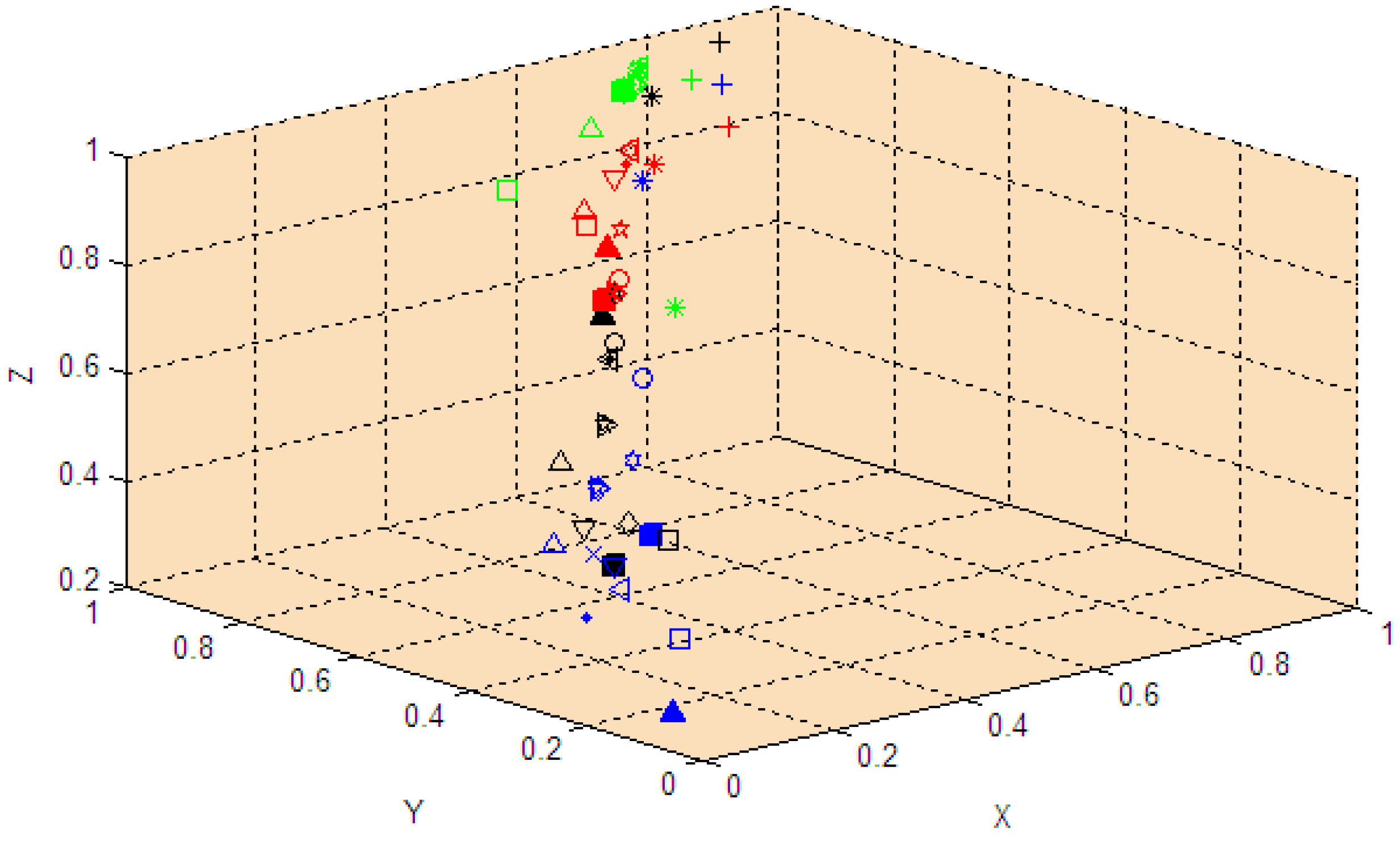


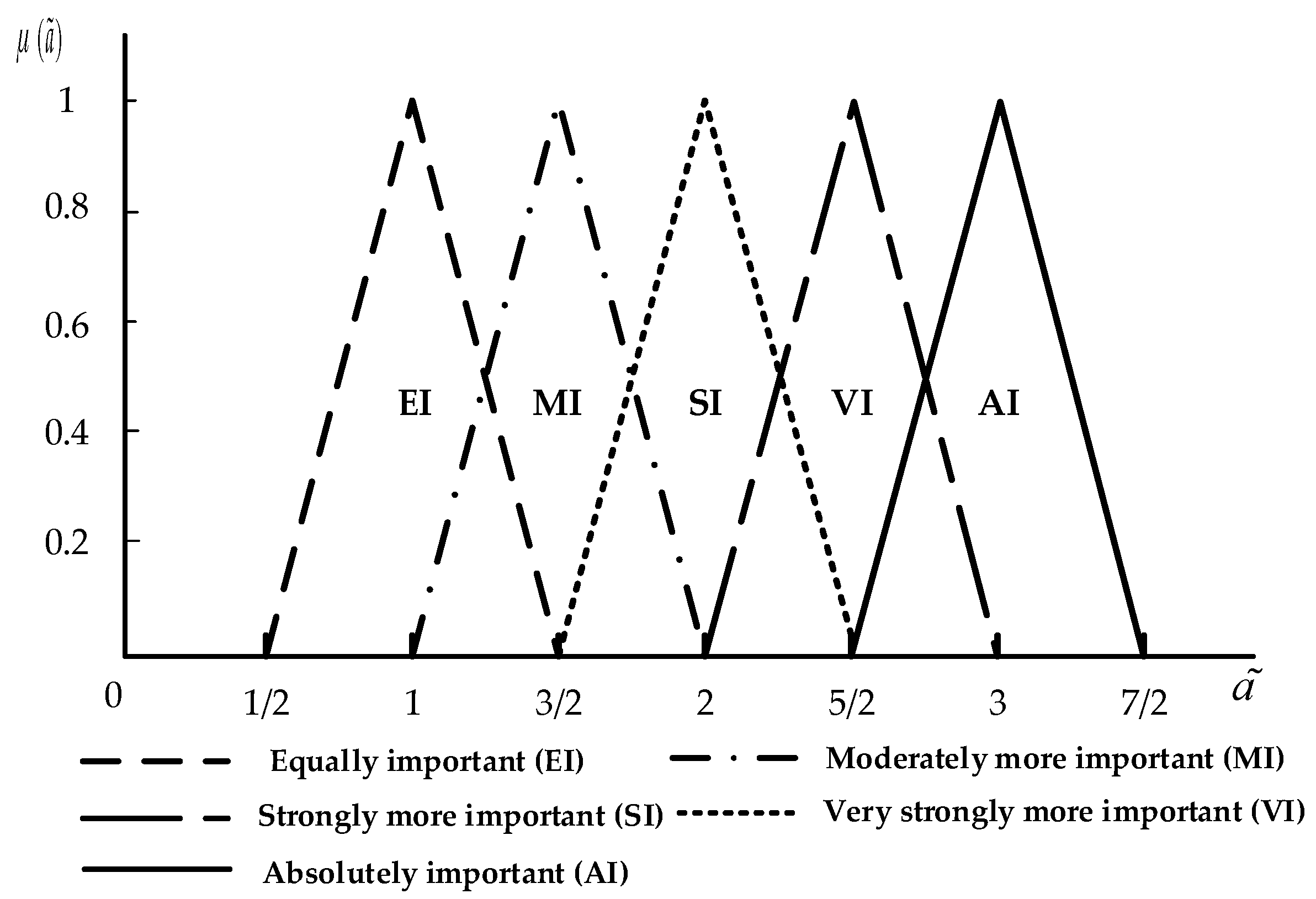
| Linguistic Terms | TFNs | Reciprocal TFNs | Meaning |
|---|---|---|---|
| Equally important (EI) | (1/2,1,3/2) | (2/3,1,2) | Criterion i is as important as criterion j |
| Moderately more important (MI) | (1,3/2,2) | (1/2,2/3,1) | Criterion i is moderately more important than criterion j |
| Strongly more important (SI) | (3/2,2,5/2) | (2/5,1/2,2/3) | Criterion i is strongly more important than criterion j |
| Very strongly more important (VI) | (2,5/2,3) | (1/3,2/5,1/2) | Criterion i is very strongly more important than criterion j |
| Absolutely important (AI) | (5/2,3,7/2) | (2/7,1/3,2/5) | Criterion i is absolutely more important than criterion j |
| n | 1 | 2 | 3 | 4 | 5 | 6 | 7 | 8 | 9 | 10 | 11 | 12 | 13 | 14 | 15 |
|---|---|---|---|---|---|---|---|---|---|---|---|---|---|---|---|
| RI | 0 | 0 | 0.52 | 0.89 | 1.12 | 1.26 | 1.36 | 1.41 | 1.45 | 1.49 | 1.52 | 1.54 | 1.56 | 1.57 | 1.58 |
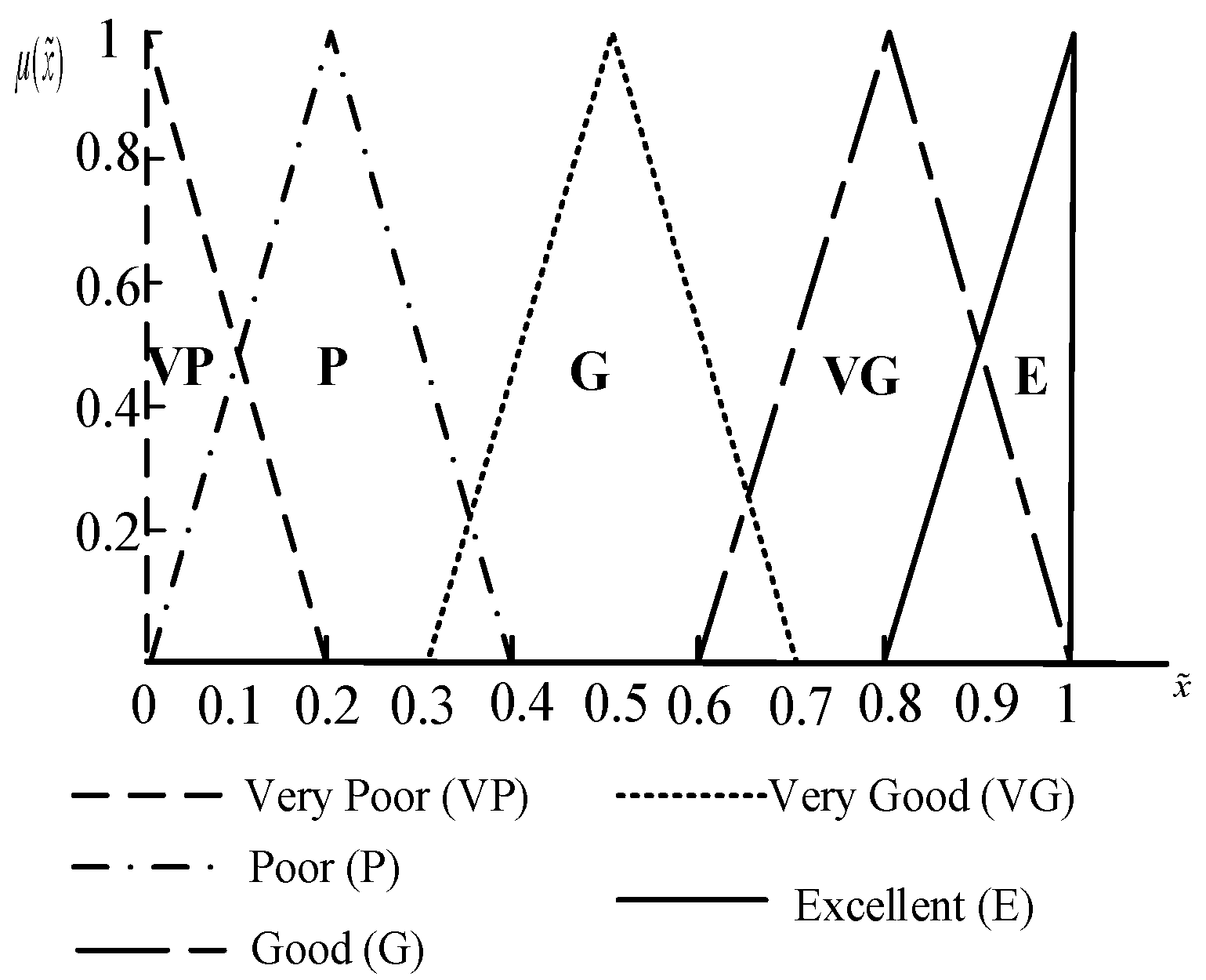
| Linguistic Terms | FTNs |
|---|---|
| Very Poor (VP) | (0,0,0.2) |
| Poor (P) | (0,0.2,0.4) |
| Good (G) | (0.3,0.5,0.7) |
| Very Good (VG) | (0.6,0.8,1) |
| Excellent (E) | (0.8,1,1) |
| CR | Goal | A1 | A2 | A3 | A4 |
|---|---|---|---|---|---|
| DM1 | 0.025 | 0.041 | 0.119 | 0.04 | 0.029 |
| DM2 | 0.036 | 0.022 | 0.019 | 0.04 | 0.037 |
| DM3 | 0.063 | 0.044 | 0.081 | 0.026 | 0.096 |
| DM4 | 0.089 | 0.05 | 0.041 | 0.016 | 0.064 |
| A1 | A2 | A3 | A4 | |
|---|---|---|---|---|
| A1 | (1.0,1.0,1.0) | (1.125,1.625,2.125) | (0.575,0.792,1.085) | (1.25,1.75,2.25) |
| A2 | (0.493,0.667,1.085) | (1.0,1.0,1.0) | (0.425,0.542,0.753) | (1.375,1.875,2.375) |
| A3 | (1.125,1.542,2) | (1.375,1.875,2.375) | (1.0,1.0,1.0) | (1.625,2.043,2.50) |
| A4 | (0.45,0.583,0.835) | (0.425,0.543,0.753) | (0.505,0.683,0.893) | (1.0,1.0,1.0) |
| C1 | C2 | C3 | C4 | C5 | |
|---|---|---|---|---|---|
| C1 | (1,1,1) | (1,1.5,2) | (0.433,0.56,0.793) | (1.082,1.475,1.875) | (1.625,2.125,2.625) |
| C2 | (0.935,1.25,1.918) | (1,1,1) | (0.365,0.45,0.585) | (0.875,1.2925,1.75) | (0.625,1.125,1.625) |
| C3 | (1.25,1.75,2.25) | (1.75,2.25,2.75) | (1,1,1) | (1.625,2.0425,2.5) | (2.125,2.625,3.125) |
| C4 | (0.825,1.0425,1.335) | (0.625,0.893,1.375) | (0.505,0.683,0.893) | (1,1,1) | (0.675,0.875,1.128) |
| C5 | (0.383,0.475,0.628) | (0.585,0.835,1.5) | (0.323,0.39,0.493) | (1.225,1.625,2.043) | (1,1,1) |
| C6 | C7 | C8 | C9 | |
|---|---|---|---|---|
| C6 | (1,1,1) | (0.725,1.043,1.418) | (0.5,0.835,1.25) | (0.625,0.96,1.375) |
| C7 | (0.893,1.25,1.793) | (1,1,1) | (0.725,0.96,1.293) | (1.125,1.543,2) |
| C8 | (0.835,1.25,2) | (0.975,1.375,1.793) | (1,1,1) | (1,1.5,2) |
| C9 | (0.793,1.168,1.75) | (0.575,0.793,1.085) | (0.5,0.67,1) | (1,1,1) |
| C10 | C11 | C12 | |
|---|---|---|---|
| C10 | (1,1,1) | (1.5,2,2.5) | (0.75,1.25,1.75) |
| C11 | (0.408,0.518,0.71) | (1,1,1) | (0.45,0.585,0.835) |
| C12 | (0.585,0.835,1.5) | (1.25,1.75,2.25) | (1,1,1) |
| C13 | C14 | C15 | |
|---|---|---|---|
| C13 | (1,1,1) | (0.5,1,1.5) | (1.125,1.625,2.125) |
| C14 | (0.67,1,2) | (1,1,1) | (1,1.5,2) |
| C15 | (0.475,0.628,0.918) | (0.518,0.71,1.168) | (1,1,1) |
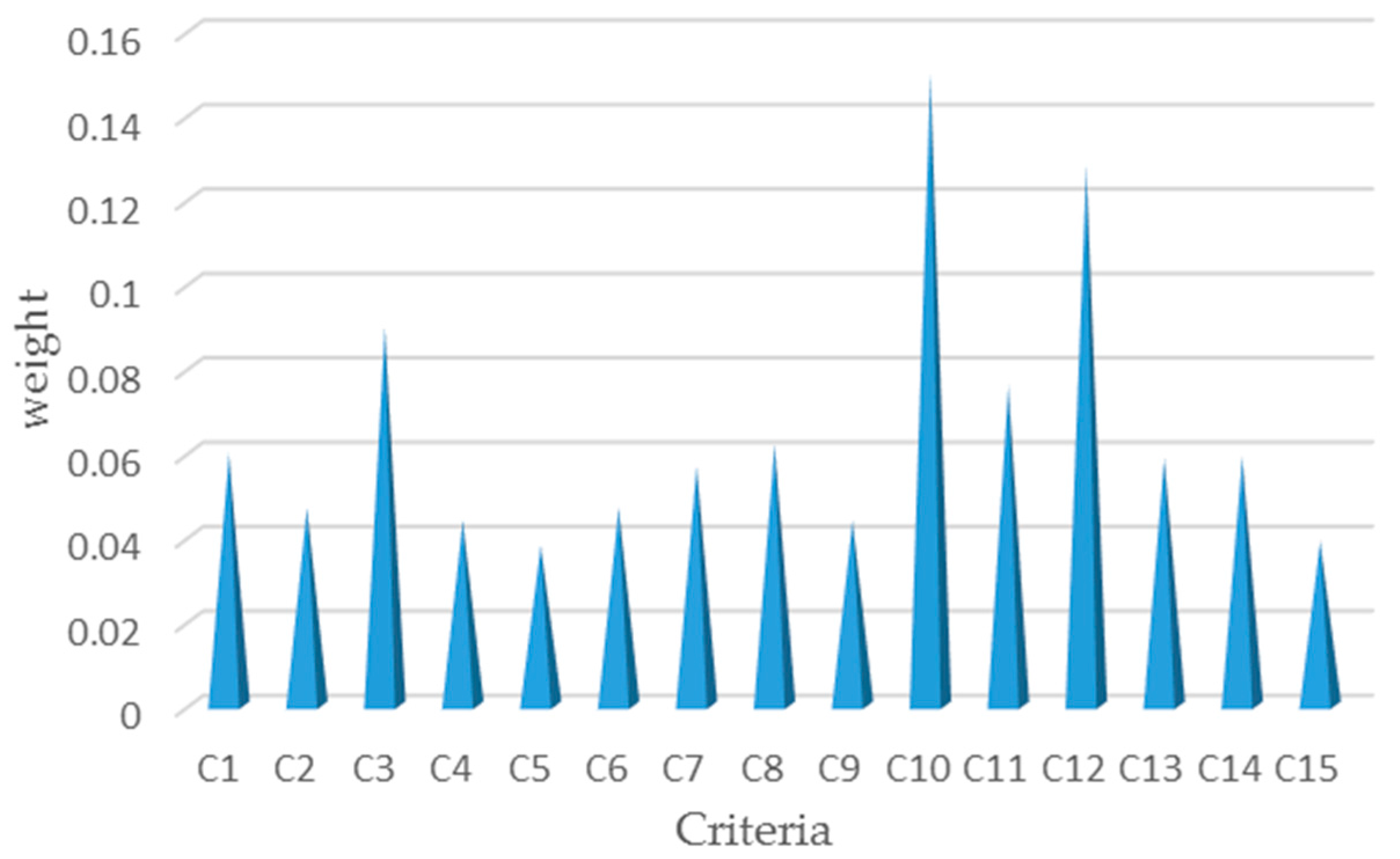
| Main Criteria | Fuzzy Synthetic Extent | Local Weight | Sub-Criteria | Fuzzy Synthetic Extent | Local Weight | Global Weight |
|---|---|---|---|---|---|---|
| A1 | (0.948,1.225,1.509) | 0.279 | C1 | (0.947,1.214,1.508) | 0.214 | 0.060 |
| C2 | (0.715,0.960,1.261) | 0.170 | 0.047 | |||
| C3 | (1.498,1.840,2.172) | 0.322 | 0.090 | |||
| C4 | (0.706,0.889,1.131) | 0.158 | 0.044 | |||
| C5 | (0.617,0.759,0.989) | 0.136 | 0.038 | |||
| A2 | (0.732,0.908,1.180) | 0.210 | C6 | (0.690,0.956,1.245) | 0.223 | 0.047 |
| C7 | (0.927,1.166,1.467) | 0.272 | 0.057 | |||
| C8 | (0.950,1.267,1.636) | 0.296 | 0.062 | |||
| C9 | (0.690,0.887,1.174) | 0.209 | 0.044 | |||
| A3 | (1.259,1.559,1.856) | 0.354 | C10 | (1.040,1.357,1.636) | 0.423 | 0.150 |
| C11 | (0.568,0.671,0.840) | 0.214 | 0.076 | |||
| C12 | (0.900,1.135,1.500) | 0.363 | 0.128 | |||
| A4 | (0.557,0.682,0.865) | 0.157 | C13 | (0.825,1.176,1.472) | 0.373 | 0.059 |
| C14 | (0.875,1.145,1.587) | 0.376 | 0.059 | |||
| C15 | (0.626,0.764,1.023) | 0.251 | 0.039 |
| j | C1 | C2 | C3 | C4 | C5 |
| (0.050,0.055,0.06) | (0.023,0.028,0.034) | (0.011,0.016,0.03) | (0.029,0.037,0.044) | (0.025,0.032,0.038) | |
| (0.043,0.047,0.055) | (0.027,0.034,0.044) | (0.21,0.054,0.09) | (0.015,0.022,0.029) | (0.006,0.013,0.021) | |
| j | C6 | C7 | C8 | C9 | C10 |
| (0.023,0.035,0.047) | (0.036,0.048,0.057) | (0.043,0.056,0.062) | (0.029,0.037,0.044) | (0.105,0.135,0.15) | |
| (0,0.012,0.024) | (0.005,0.014,0.026) | (0.009,0.022,0.034) | (0.007,0.015,0.024) | (0.011,0.034,0.064) | |
| j | C11 | C12 | C13 | C14 | C15 |
| (0.049,0.064,0.076) | (0.09,0.116,0.128) | (0.037,0.049,0.059) | (0.037,0.049,0.059) | (0.028,0.036,0.04) | |
| (0.017,0.028,0.044) | (0,0.026,0.051) | (0,0.003,0.016) | (0.01,0.016,0.029) | (0.003,0.011,0.019) |
© 2016 by the authors; licensee MDPI, Basel, Switzerland. This article is an open access article distributed under the terms and conditions of the Creative Commons Attribution (CC-BY) license (http://creativecommons.org/licenses/by/4.0/).
Share and Cite
Dong, J.; Huo, H.; Guo, S. Demand Side Management Performance Evaluation for Commercial Enterprises. Sustainability 2016, 8, 1041. https://doi.org/10.3390/su8101041
Dong J, Huo H, Guo S. Demand Side Management Performance Evaluation for Commercial Enterprises. Sustainability. 2016; 8(10):1041. https://doi.org/10.3390/su8101041
Chicago/Turabian StyleDong, Jun, Huijuan Huo, and Sen Guo. 2016. "Demand Side Management Performance Evaluation for Commercial Enterprises" Sustainability 8, no. 10: 1041. https://doi.org/10.3390/su8101041
APA StyleDong, J., Huo, H., & Guo, S. (2016). Demand Side Management Performance Evaluation for Commercial Enterprises. Sustainability, 8(10), 1041. https://doi.org/10.3390/su8101041