Abstract
Currently, oversupply coal and coal-based power in China poses a great challenge to energy structure optimization and emissions reduction. The energy industry, however, is closely linked to the financial sector. In view of this, using a non-linear Panel Smooth Transition Regression (PSTR) model, this paper examines the threshold effects of financial developments on energy supply structures for 17 energy supply provinces in China observed over 2000–2014. The main results are: (1) The ratio of coal supply (LCSR) specification is seen to be a four-regime PSTR model with added value in the financial industry/GDP (LFIR) as the threshold variable. The LFIR and LCSR show a positive correlation, and the elastic coefficients change between 0.02 and ~0.085; the impact of financial institutions’ loan balance/GDP (LLAN) on LCSR takes on an inverse U-shaped curve: first positive, then negative, and again positive with the financial crisis in 2008 as the turning point; (2) The ratio of thermal power generation (LTPG) specification is seen to be a two-regime PSTR model with investment in the coal industry/GDP (LCIR) as the threshold variable. Results show that LFIR has a negative effect on LTPG, and the coefficients in the low regime tend to be 0.344%, then gradually decrease to 0.051% in the high regime. The influence of LLAN on the LTPG is positive before and negative after the financial crisis. The influence of the foreign direct investment GDP proportion (LFDI, the degree of financial openness) on the LCSR and LTPG both remain negative. Therefore, in the process of formulating energy conservation policies and adjusting energy-intensive industrial structures, the government should fully consider the effect of financial developments.
1. Introduction
Being an important driving force of the world’s economic growth, the future development of the Chinese economy is of great concern around the world. Starting in 2012, the Chinese economy entered the “new norm”, which means the growth rate of GDP fall from high speed to middle–high speed, and the optimization and upgrading of economic structure should be the priority for the next five-year blueprint. Against this background, supply-side reform was put forward by the authorities before starting on the 13th Five-year Plan. As the blood of the modern industrial economy, structural reform of the supply side in the energy sector is paid specific attention. Resolving the excess supply of coal production and electricity generation from coal are listed as the top two tasks of structural reforms for energy supply, so as to promote the energy supply structure becoming cleaner.
Although oil, natural gas, and water consumption and production have increased rapidly in recent years, coal is still the dominant energy source in China. Coal accounts for about 74% of China’s primary energy production and 66.03% of energy consumption in 2015 (National Bureau of Statistics of China (NBSC), 2016) [1]. Thermal power generation, of which coal is the main energy source in China, accounted for 75.56% of the electricity production in 2014 (National Bureau of Statistics of China (NBSC), 2015) [2]. However, the demand for steel and cement has been decreasing in this new normal economy, thus leading to a decreasing coal demand (due to one-quarter of coal traditionally being used in the steel and cement industry). In 2014, coal overcapacity reached 646 million tons. In 2015, the operating time for thermal power equipment was only 4329 h, reaching the lowest rate of thermal power equipment utilization since 1978. Based on the thermal power break-even point of 5500 h, there is an excess of over 20%. In addition, the increasingly severe air pollution situation is putting pressure on China to reduce its coal production and generate electricity from coal. Thus, it is important to investigate the energy supply, especially the coal supply.
This paper aims to make a contribution to the energy supply structure research from the perspective of financial development. To date, the literature has seldom focused on the relationship between financial development and energy supply, but the potential nexus is not difficult to grasp. Just as the People’s Bank of China puts it, the financial sector plays an important role in the reform of supply-side structure; banks should continue providing loans for deserving businesses in the steel, nonferrous industry, building, shipbuilding and coal industries, but withdraw credit for related “zombie” companies [3]. In reality, energy production has been closely related with the financial sector in the last few decades in China, because many mining enterprises initially borrowed money for preliminary investment in mineral exploration. However, if these enterprises were to go into liquidation, the bad debt at the banks would increase sharply. Banks would continue lending to these zombie enterprises rather than expose their bad debt. Now, as coal prices fall and there is an excess coal production capacity, the bad debts incurred by the financial system have become an ever-present problem. Theoretical models also show that financial instruments, markets, and institutions may arise to mitigate the effects of information and transaction costs. Thus, financial systems may influence saving rates, investment decisions, technological innovation, and, hence, production decisions for energy enterprises [4]. The function of resource allocation in financial systems can also lead to energy structure changes. For instance, guided by a credit fund flow and affected by equity asset prices, energy enterprises can adjust their future production structures. Therefore, this paper aims to explore the relationship between financial developments and energy supply structure for 17 energy Chinese provinces from 2000 to 2014 using an empirical model, intending to find a general rule so as to provide a reference and advice for the reform of China’s energy supply-side structure.
2. Literature Review
2.1. The Evolvement of Financial Development Indicators
The first quantitative indicator measuring financial development is the Financial Interrelation Ratio (FIR), which was put forward by Goldsmith (1969) [5]. The simplified formula is FIR = Gross financial assets/GDP, and the total financial assets is the sum of M2, total stock value, the balance of treasuries, financial bonds, and corporate bonds. In fact, FIR is more often used to analyze the change of financial structure. In the 1990s, the wave of empirical research on financial development and economic growth forced scholars to create new financial indicators. King and Levine made a great contribution to it, making up the shortfall of Goldsmith’s indicator [6]. In order to investigate the relationship between financial development and economic growth, they took a sample of 77 countries from the period 1960–1989, and controlled for other potential factors that might impact on economic development. The following financial development indicators are used in their research: (1) the ratio of liquid liabilities of financial intermediary to GDP (in reality, this is always measured by M2/GDP); (2) CMB/(CMB + CEB), CMB means the total assets of commercial banks for one country, and CEB is the assets of central bank for one country. The indicator reflects financial system’s efficiency in a country, because commercial banks are usually believed to be more efficient in capital allocation than central banks; (3) the ratio of domestic credit to private sector/GDP is also used to denote financial efficiency. However, the shortcomings of their findings are the sole focus on the banking sector, and ignoring the influence of other financial markets like stocks and bonds. In 1998, Levine and Zervos supplemented several stock indexes, including stock market capitalization to GDP, stock market value traded to GDP, and stock market turnover [7,8]. Nowadays, cointegration and causality tests are still mostly used to investigate the long-running relationship among financial development, economic growth, and energy consumption [9,10,11,12,13]. In addition to the financial indicators put forward by King and Levine [6], they constructed other banking indicators like the ratio of deposit money bank assets to GDP, the ratio of financial system deposits to GDP, the ratio of liquid liabilities to GDP, and stock market variables like the number of listed companies per 10,000 people.
2.2. Why Does Non-Linear Analysis Matter in the Energy Supply Model?
As mentioned in Section 1, previous literatures have not investigate the relationship between financial development and energy supply. Only a few studies threw some light on the relationship between economic growth and energy supply, and long-run relationships have been detected between GDP and energy supply in Malaysia [14] and China [15] by causality testing. In fact, a non-linear relationship has certainly been detected between financial development and economic growth (energy consumption). Deidda and Fattouh (2002) showed that finance has a nonlinear effect on economic growth by means of a panel smooth regression (PSTR) model with the income level used as the transition variable. The financial development is found to be significant only in high-income countries [16]. From a sample of 71countries between 1960 and 2004, Jude suggests the existence of threshold effect in the nexus between finance and growth, with financial development as the transition variable affecting the non-linearity the most [17]. Doumbia relies on the PSTR model, and highlights the financial development that supports economic growth in low-income and lower-middle income countries by enhancing saving and investment behavior. However, in more developed economies, the impact of financial development tends to be weaker [18]. By establishing a Panel Threshold Regression (PTR) model, Chang found an asymmetric threshold effect existing in low-income and high-income countries. In the low-income regime, energy consumption increases with banking developments but slightly declines with stock market development in advanced economies, especially in high-income countries [19]. Lee and Chiu identify a nonlinear relationship between electricity consumption, real income level, electricity price, and temperature by means of PSTR model [20], and then apply a newly developed PSTR model with the error-correction term (PSECM) to estimate the non-linear relationship between energy consumption, real income, and real energy prices for 24 OECD countries [21]. In addition, it has been found that the financial development could lead to environmental degradation [22] and an increase in greenhouse gas emissions (Zhang [23]). According to output theory, GDP signifies the gross domestic production within a specific period; in the same way, energy supply signifies the production in the energy sector, which can also denote an output like GDP. Now that financial development can account for economic growth to some degree, it may also explain the energy supply. Therefore, this work intends to examine the existence of nonlinearity in the nexus between financial development and energy supply structure by means of a PSTR model developed by Gonzalez et al. (2005) [24]. In both Panel Threshold Regression (PTR) and panel Markov regime-switching (PMRS) models, regime switching is assumed to be abrupt with dispersion, so seldom conforms to the actual laws of economics [25]. Combining the PTR model and the Smooth Transition Regression (STR) model (for time series data), Gonzalez et al. developed the PSTR model, specifying a transition function smoothly changing from 0 to 1 continuously in the non-linear part of the PSTR equation. This approach presents advantages over the other nonlinear models. The PSTR model permits a smooth and continuous regime transition by considering several potential thresholds; thus, the PSTR specifications allow the finance–energy supply structure coefficients to vary not only between provinces, but also with time. This provides a simple way to appraise the heterogeneous relationship between finance and energy supply structure with time and according to provinces.
The structure of this paper is as follows: Section 3 gives details of the data sources and the variables selected in this paper and PSTR model introduction; Section 4 is the empirical process, encompassing four parts: unit root test, non-linear test and transition regime determination, PSTR model estimation, and feature analysis of transition function. Section 5 is the discussion, in which we analyze the time-varying impact of financial development indicators on the ratio of coal supply and thermal power generation. Section 6 presents the conclusions.
3. Data, Variables, and Model Introduction
3.1. Data and Variables
The panel dataset is yearly and covers the period from 2000 to 2014 (according to data availability) for 17 provinces with ample energy resources. The 17 provinces are Anhui (AH), Gansu (GS), Guangxi (GX), Hebei (HA), Heilongjiang (HL), Henan (HE), Hubei (HB), Jilin (JL), Jiangsu (JS), Liaoning (LN), Inner Mongolia (NM), Ningxia (NX), Qinghai (QH), Shandong (SD), Shaanxi (SN), Sichuan (SC), and Xinjiang (XJ). The data are derived from the China Statistical Yearbook and statistical yearbooks for the relevant provinces [26], the China Financial Yearbook [27], the wind database [28]. According to the National Energy Administration, resolving the excess supply of coal production and electricity generation from coal are listed as the top two tasks of structural reforms for energy supply. Therefore, the ratio of coal production to total energy production (LCSR) and the ratio of thermal power generation to gross generation (LTPG) are used as two variables to measure the energy supply structure.
The financial developments in this paper are proxied by the ratio of added value in the financial industry to GDP (LFIR), the ratio of financial system loan balance to GDP (LLAN), and the ratio of foreign direct investment to GDP (LFDI). As mentioned in Section 2, this refers to M2, total stock value, the balance of treasuries, financial bonds, and corporate bonds when calculating the financial interrelation ratio (FIR). However, the related data are not published in a single province in China. Since that FIR is used to signify the total financial activities during one period, this paper replaces the total financial assets with the added value in the financial industry. Thus, we use the ratio of the added value in the financial industry to GDP to represent the financial correlation ratio and reflect the general financial industry development degree in a province.
According to Section 2.1, the ratio of domestic credit to private sector/GDP, the ratio of deposit money bank assets to GDP, and the ratio of financial system deposits to GDP et al. are widely used to measure banking developments. Due to the limitation of Chinese statistics, we can only find the yearly balance of loans, so we use the ratio of financial system loan balances to GDP to assess the scale of the credit market expansion in China. As financial institution loans are the main capital sources for energy production investment in energy-producing provinces, the flow of credit funds from financial institutions directly affects energy supply. Larger values indicate that more funds are available for loaning out, which should stimulate consumption, investment, economic growth, and energy demand and production.
Foreign direct investment/GDP (LFDI) is another financial development indicators used in this paper. Foreign direct investment can not only stimulate economic growth through technology transfer and diffusion, productivity gains, and managerial skills [29], but also reduce energy consumption with respect to non-renewable sources and increase the consumption of renewable sources [30,31]. In this way, the energy supply structure might be impacted. According to Beck and Kun, financial openness should also be taken into account when measuring financial development [32], and Sun et al. use foreign direct investment to proxy financial openness [33]. Thus, this paper adopts Sun’s method to denote the openness of finances.
The investment in the coal mining and washing industry/GDP (LCIR) is another factor influencing the coal supply structure. Energy investment is the material basis of the formation of the energy supply system, and is the fundamental guarantee of the stability, economics, and clean energy supply [34]. The increase of investment in the coal industry can promote the increase of the coal supply.
3.2. PSTR Model Specification
Following González et al. (2005) [24], the basic definition for the two-regime switching model is as follows:
where represents the number of cross sections, represents the time duration, represents an explained variable, is an explanatory variable in dimension, and and represent the individual fixed effect and the estimated residual error. The transition variable continuously ranges from (0, 1), changing with the threshold variable , so the corresponding regression coefficient is between and . Logistic functions from Granger and Teräsvirta [35] and Teräsvirta [36] were used as the transition functions in this paper.
where is the slope parameter for the transition function (transition rate) that determines the regime switching speed and smoothness, i.e., the speed of the transition from one regime to another; is the transition (threshold) variable. In this paper, we consider a first lagged value of the explanatory variable as a potential threshold variable in order to avoid a simultaneity issue [37]. represents a vector of the position parameter in dimension. To meet the model identification needs, the limits were set at . In practice, only if or can we capture the nonlinearities due to regime switching. When and , the transition function becomes an indicator function. When > , the transition function tends to equal 1; otherwise, the transition function tend to equal 0. When the transition function becomes constant and the model collapses into a homogenous or linear panel regression model with fixed effects (the so-called “within” model).
For the non-linearity test, the null hypothesis is H0: = 0, expressing no regime-switching effect in the model. However, as mentioned above, the model collapses into a linear panel regression model under the null hypothesis, thus the classical tests have no standard distribution, which results in the so-called Davies Problem [38]. One way to solve this problem is to replace the transition function with its first-order Taylor expansion around the null hypothesis = 0 [20]. When m = 1 and m = 2, respectively, the first-order Taylor expansions around = 0 of the transition function are:
After reparameterization, the auxiliary regression based on m = 1 and m = 2, respectively, can be written as:
So, the first-order Taylor expansion depends only on since m = 1 and the parameter associated to is a multiple of the slope parameter. m = 2 depends on and , where , and is the remainder of the Taylor expansion. Let , then testing linearity (no regime-switching effect) against the PSTR model is meant simply to test the null hypothesis H0: in these auxiliary regressions. According to Colletaz and Hurlin [39], the three nonlinear statistical tests are as follows:
Here, SSR0 is the panel sum of squared residuals under H0 (linear panel model with individual effects), SSR1 is the panel sum of squared residuals under H1 (PSTR model with two regimes), and K is the number of explanatory variables. If the linearity hypothesis is rejected, we can continue testing for no remaining nonlinearity to explore whether there are another transition functions. The test will not stop until the null hypothesis cannot be rejected.
4. Empirical Analysis
4.1. Unit Root Test
For the sake of avoiding spurious regression, the unit root test is conducted on each variable after taking natural logarithm. By means of the Levin–Lin–Chu (LLC) test, the Fisher–ADF test, and the Fisher–PP test, all variables are proven to be stationary series. The LLC tests are listed in Table 1. The original LLC test hypothesis is that cross section panel data series have the same unit root, and the alternative hypothesis is that there is no unit root for any cross section series. Based on the statistics and P value in the unit root test shown in Table 1, there is no unit root for the level value of the cross section series. After Pedroni and Kao tests, a co-integration relationship is proven to exist between the explained variables and explanatory variables, indicating the existence of a long-term balance relationship. Therefore, it is appropriate to undertake further study on the relationship between financial development and energy structures.

Table 1.
Unit root test results.
4.2. Nonlinearity Test and Transition Regime Determination
Before estimating the PSTR model, it is necessary to conduct a non-linearity test so as to check if it is proper to build a PSTR model. As mentioned in Section 3.2, it is suggested to use the first-order value of explanatory variables as potential transition variables, so we apply LFIRit-1, LLANit-1, LFDIit-1, and LCIRit-1 to the non-linear test. There are three targets in the process of non-linear testing: (1) examine whether there is non-linearity between financial development indicators and energy supply structures; (2) pick the optimal transition variable; and (3) determine the number of transition functions and location parameters. The testing procedure works as follows. First, test a linear model (r = 0) (r is the number of transition function) of the LCSR and LTPG specifications against a model with one threshold function (r = 1). If the null hypothesis H0 is rejected, this indicates the existence of nonlinearity of the model. Then proceed to the second step: test for remaining non-linearity and determine the number of transition functions. Test a one threshold (r = 1) model against a double threshold model (r = 2). The procedure is continued until the null hypothesis (H0: r = r*) is not rejected, and then r* is the optimal number of transition functions. For each specification, we compute the LM, LMF, and LRT statistics for the linearity tests. Since previous studies have documented that the F-version of the test has better size properties in small samples than the asymptotic-based statistic [7], we only report the LMF statistic of LCSR and LTPG specifications in Table 2. The LMF has an asymptotic distribution under H0, where m is the number of location parameters and K the number of explicative variables. In our specifications we have K = 4.
Table 2.
LMF Tests for nonlinearity tests and determination of the transition variables.
According to Table 2, the linear tests (H0: r = 0 vs. H1: r = 1) for all four models proved the existence of nonlinearity in LCSR and LTPG specifications. For LCSR specifications, the subsequent tests show that Model 1 and Model 2 are four-regime models, Model 3 is a three-regime model, and the number of regimes in Model 4 depends on the number of location parameters. Furthermore, the strongest rejection of the null hypothesis of linearity (H0: = 0 vs. H1: = 1) is obtained from Model 1 whenever the position parameter m = 1 or m = 2. According to González et al. (2005) [23], the variable that most strongly rejects linearity should be selected as the transition variable. Thus, in the LCSR specification, the optimal model would be Model 1, which uses the lagged one value of the ratio of added value in the financial industry to GDP (LFIR) as a threshold variable with the number of transition function r* = 3. For LTPG specification, the subsequent tests show that all four models are two-regime models. The strongest rejection of the null hypothesis of linearity (H0: = 0 vs. H1: = 1) is obtained from Model 4 whenever the position parameter m = 1 or m = 2; thus, the optimal model would be Model 4, which uses the lagged one value of the investment in the coal mining and washing industry/GDP (LCIR) as a threshold variable with the number of transition function = 1.
Table 3 shows the examined results for choosing the number of location parameter with m = 1 or m = 2. According to Colletaz and Hurlin [40], the AIC and BIC criteria are used to determine the optimal number of location parameter for each model. It is proposed to choose the optimal that minimizes the AIC and BIC. For the LCSR specification, when m = 1, the AIC and BIC values are relatively smaller and the optimal number of transition functions are = 3, so the model format is to be set as = (3, 1), with LFIRit-1 as the transition variable. For the LTPG specification, when m = 1, the AIC and BIC values are relatively smaller, and the corresponding optimal number of transition functions is = 1, thus, the model format is to be set as = (1, 1), with LCIRit-1 as the transition variable.
Table 3.
Determination for the number of location parameter.
4.3. PSTR Model Estimation
Based on the non-linear test results presented in Section 4.2 and Equation (1) in Section 3.2, we set the final LCSR and LTPG equations as follows:
Of which,
Of which,
In the LCSR specification, represents the fixed effect on the energy supply structure except for the explanatory variables, is the random error term. () represents the linear estimated coefficients, and , and represent the nonlinear estimated coefficients. In the LTPG specification, is the fixed effect, is the random error term. () represents the linear estimated coefficients, and represents the nonlinear estimated coefficients.
The Nonlinear Least Square (NLS) is adopted to estimate the parameters. Before the parameter estimations, a grid search method is adopted to determine the preliminary values for the transition rate and the position parameter . To guarantee accuracy and to save program operating time for parameter estimation, the number of iterations is set at 20,000. The parameter estimation results for the two specifications are shown in Table 4 and Table 5.
Table 4.
PSTR model estimation results for the impact of financial developments on LCSR.
Table 5.
PSTR model estimation results for the impact of financial developments on LTPG.
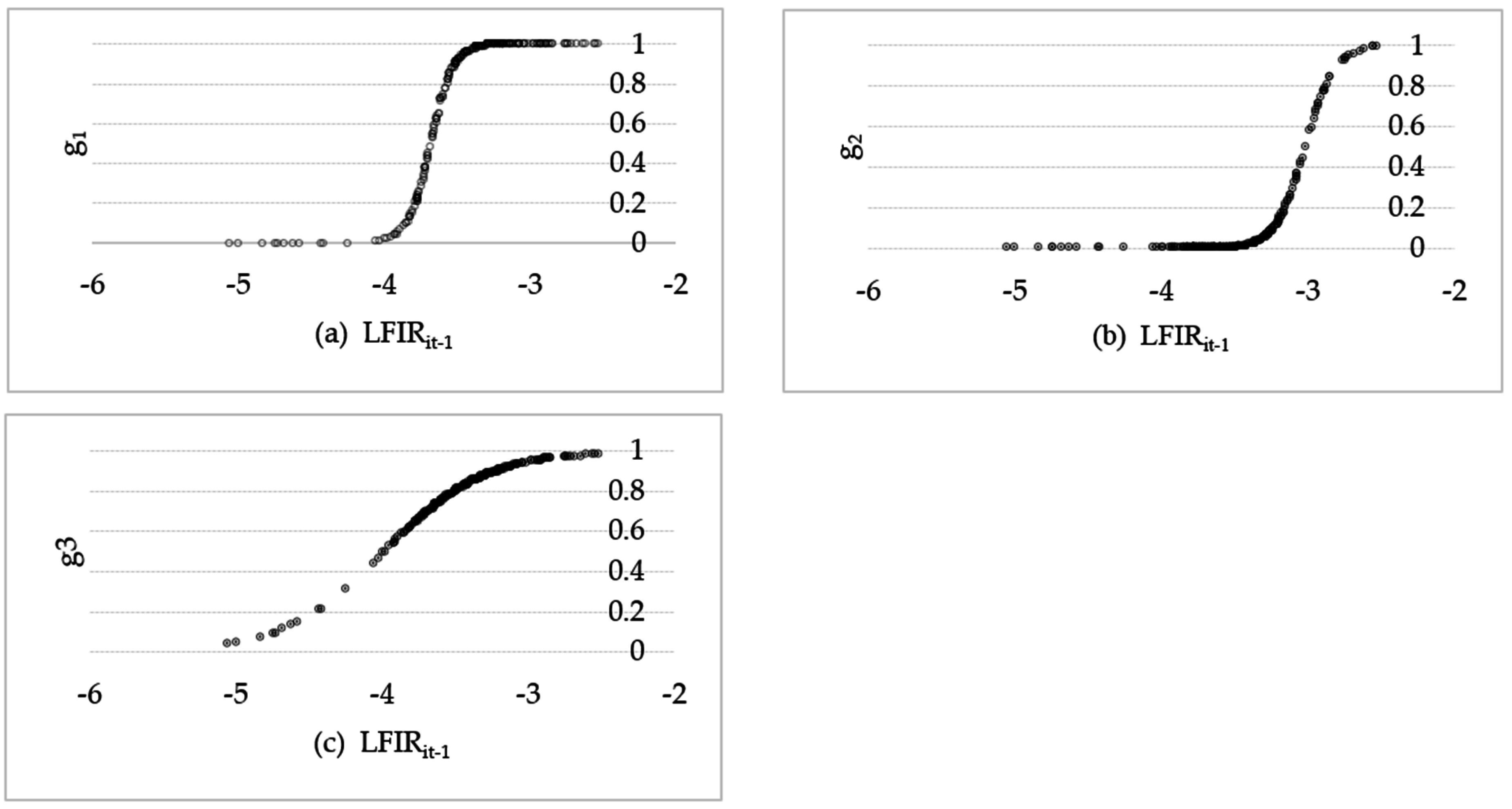
In LCSR specification, the coefficients in Regime 1 stand for the linear part. Regime 2, Regime 3, and Regime 4 are the non-linear parts. In Regime 2 for the first transition function, the estimate parameters are significant except for LLAN, and the slope parameter is 13.027, the location parameter is –3.677. The quite big slope parameter indicates that the transition speed rate from one regime to another is prompt. This can also be seen in Figure 1a, where we can see that the tendency of the transition function is quite sharp. Most circles (which signify the transition function values) are bound to 0.9~1. In Regime 3 for the second transition function, the slope parameter is 9.97 and the location parameter is –3.014. As seen in Figure 1b, most of its circles standing for the transition function values distribute around 0~0.2. Contrary to the transition function g1, transition function g2 is nearly a zero indicator function. In Regime 3 for the third transition function, the slope parameter and corresponding location parameter are 2.9 and −3.989, respectively. In Figure 1c, the transition function has a relatively gradual incline, and the majority of threshold variables are larger than the location parameter −3.989; almost all of the transition functions g3 range from 0.5 to 1.
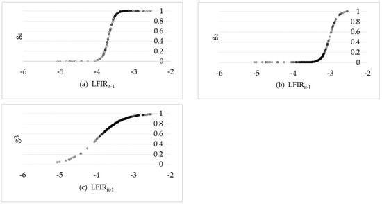
Figure 1.
Transition function for LCSR specification. (a) The first transition function with slope parameter equaling to 13.027; (b) the second transition function with slope parameter equaling to 9.97; (c) the third transition function with slope parameter equaling to 2.90.
The LCSR specification contains three transition functions with the ratio of added value in the financial industry to GDP (LFIR) as the transition variable. Because we take the logarithm for each variable during model estimation, now for the convenience of analysis, we calculate the exponential location parameter value e–3.989 = 0.0185, e–3.677 = 0.0253, e–3.014 = 0.0491. According to , we can calculate the threshold value in each non-linear regime. We find the elastic coefficient for LFIR ranges from 0.049 to ~0.095, indicating that the expansion of the whole financial scale is not helpful for the reduction of coal supply structure. The elastic coefficient for LLAN changes from −0.498 to −0.077, meaning that the increase of credit proportion exerts a reduction effect on the coal supply structure. In addition, when the LFIRit-1 > 0.491, the elasticity increases with the increase of LFIR. When LFIRit-1 < 0.0185, the elastic coefficient for FDI is small but negative, but with the increase of LFIRit-1, the elastic coefficient for FDI gradually increases. In the regime 4 with LFIRit-1 = 0.0491, the coefficient is −0.126. It can be deduced that as the financial sector plays a more and more important role in the future, foreign direct investment will make a greater contribution to decreasing the coal supply. The elastic coefficient for LCIR is negative when LFIRit-1 < 0.0253, and then turns positive afterwards. Based on the coefficient analysis above and considering that the ratio of added value in the financial sector/GDP will continue to increase in the future, banks should lend more money to qualified coal production businesses so as to squeeze out the inefficient enterprises. On the other hand, local governments should introduce more foreign direct investment, such that the local energy business can learn about advanced technology and management skills, and improve the energy utilization efficiency.
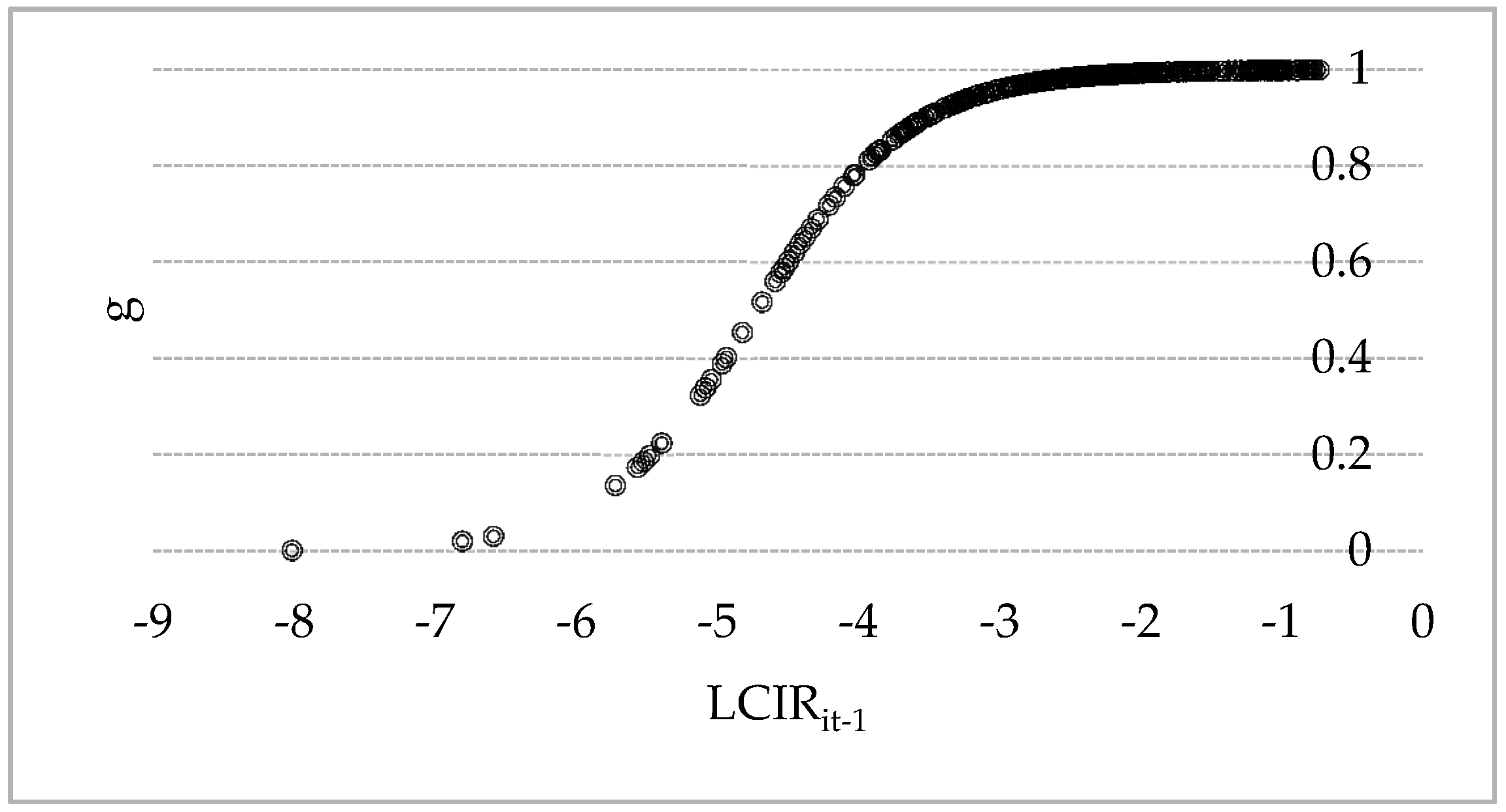
The LTPG specification is a two-regime PSTR model with investment in the coal mining and washing industry/GDP (LCIR) as the threshold variable. As can be seen in Table 5, the slope parameter is 1.840, and the location parameter is −4.724. The small slope parameter shows that the transition function changes smoothly and slowly, which can also be seen in Figure 2. In addition, most of the values of transition variables are greater than the estimated location parameter 0.0089 (e–4.724 = 0.0089), resulting in most of the circles standing for transition function values greater than 0.5 and distributing around 0.8~1. According to , the elastic coefficient for LFIR at LCIRit-1 = 0.0089 equals −0.1975, meaning that a 1% increase in the LFIR will lead to a 0.1975% reduction in the ratio of thermal power generation. With the increase of LCIRit-1, the reduction effect will be greater. To identify the exact threshold value from positive to negative of the transition function for LLAN, we transform the format of the transition function to obtain the turning point, and calculated 0.0374, indicating that when the coal mining and washing industry investment proportion (LCIR) is larger than 0.0374, there is a negative correlation between LLAN and LTPG. Conducting the same conversion for the transition function for LFDI, we achieve the turning point at 0.0234. This means when LCIRit-1 is larger than 0.0234, the elastic coefficient between LFDI and LTPG is negative, and vice versa. The coefficients for LCIR are not significant in either regime, so we did not perform a detailed analysis. Based on the coefficient analysis above, augmented investment in the coal mining and washing industry is encouraged. With the increase of LCIR, the financial sector, credit market, and foreign investors will have a reduction effect in the proportion of thermal power generation. More detailed analysis of the impact of financial development and LCSR and LTPG specifications will be given in Section 5.
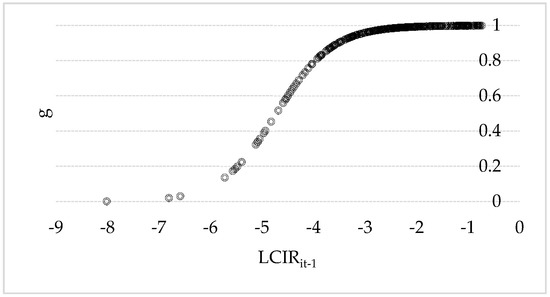
Figure 2.
Transition function for LTPG specifications.
5. Discussion
5.1. The Time-Varying Elasticity Analysis of the LCSR Specification
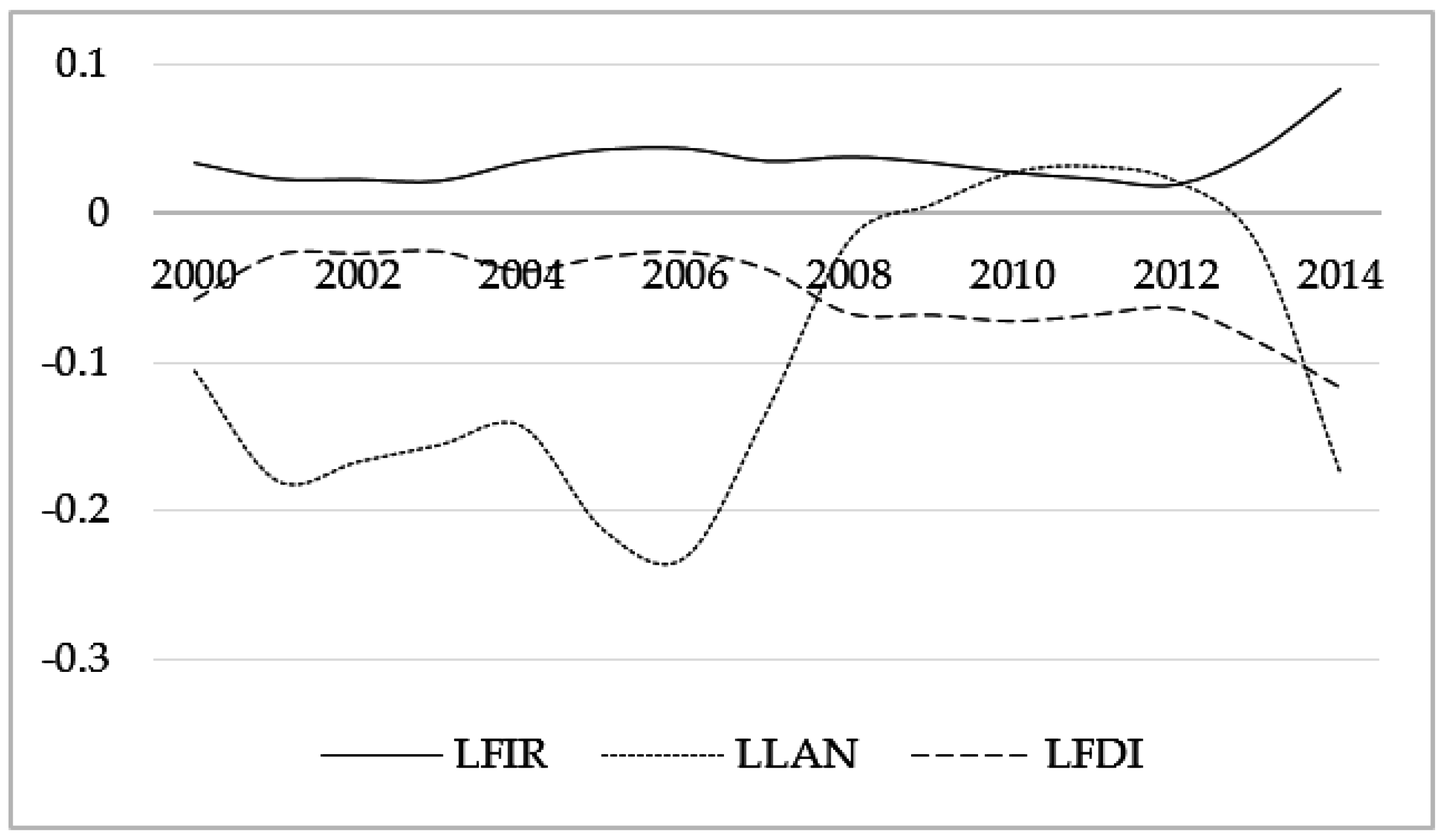
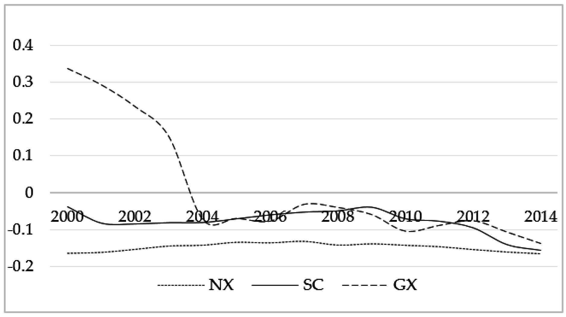
The LCSR specification is a four-regime PSTR model with the added value in financial industry/GDP (LFIR) threshold variables, indicating that LFIR is the most important influential factor resulting in the non-linear relationship in LCSR specification. By summing up the elastic coefficients in the same year in every region and calculating the average values, we gain the time-varying elasticity between financial development and the coal supply structure when the regional differences are disregarded. As shown in Figure 3, LFIR and LCSR show a positive correlation, and the elastic coefficients change between 0.02% and ~0.085%; the impact of LLAN on LCSR takes on an inverse U-shaped curve: first positive, then negative, and again positive with the financial crisis in 2008 as the turning point. The influence of LFDI on LCSR remains negative, ranging from −0.116% to −0.254%.
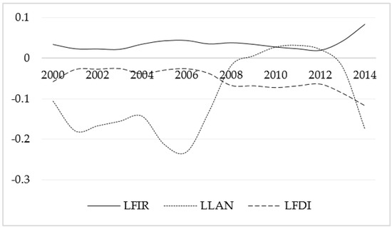
Figure 3.
Time-varying elasticity between financial development indicators and LCSR.
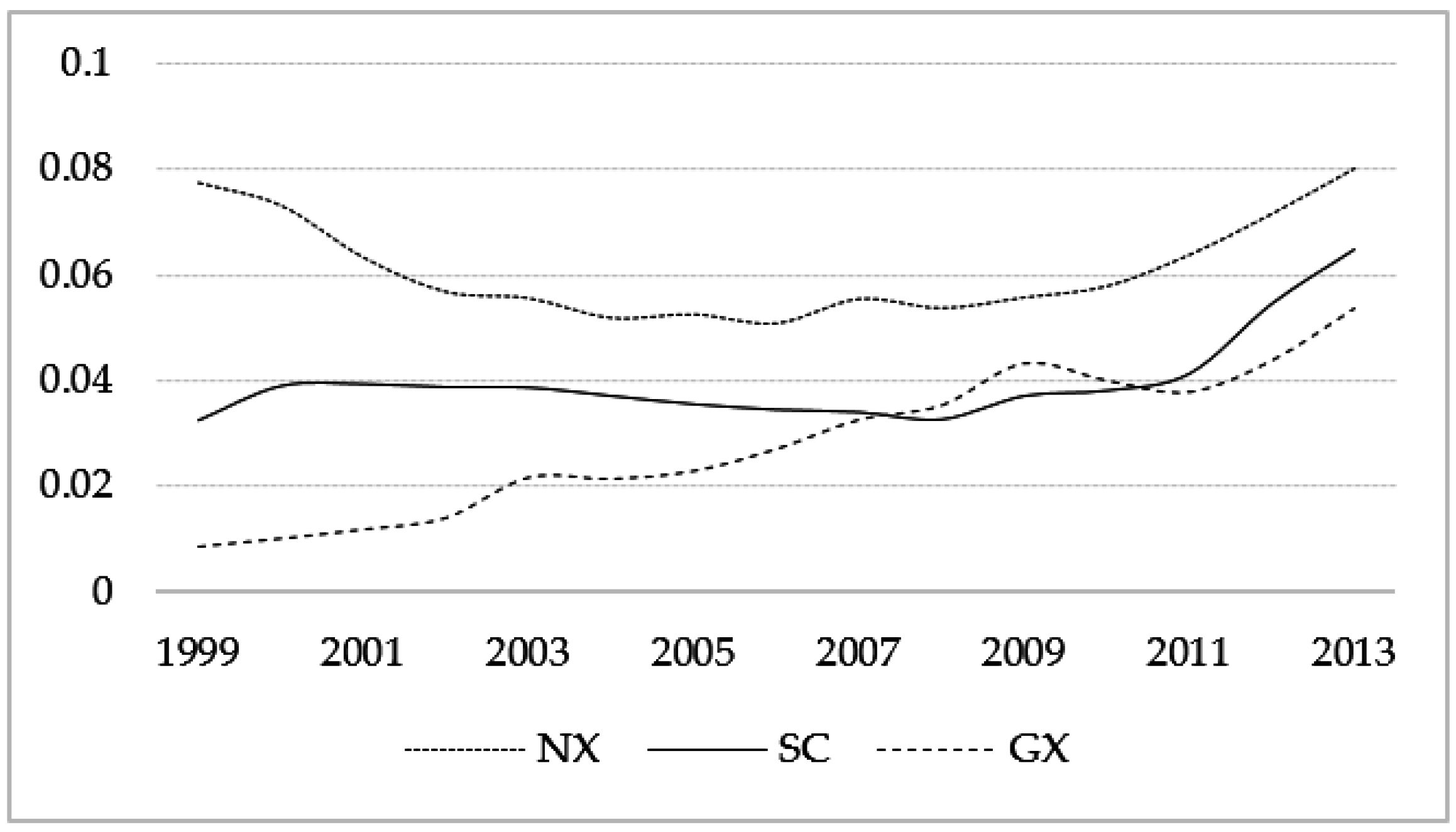
In order to detect the regional difference effect, this paper selects three provinces, Ningxia (NX), Sichuan (SC), and Guangxi (GX), to stand for different levels of financial development. Figure 4 presents the variation trend of the added value in financial industry (%GDP) (LFIR) in the three provinces. In Ningxia, the LFIR ranges from 5% to 8%, standing for the higher degree of financial development. In Sichuan, the range scope is 3% to 6.5%, representing the middle level. Before 2012, the added value in the financial industry (%GDP) fluctuated within a narrow range (3%~4%); from 2012 to 2014, it experienced a rapid increase and rose to 6.5% within two years. In Guangxi, the added value in the financial industry (%GDP) increased continuously. The range is quite large, from 1% to 5%, standing for a lower but rapid growth financial development level.
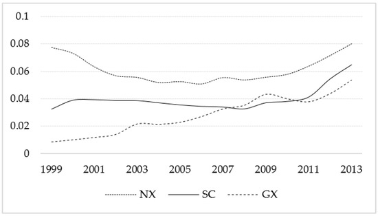
Figure 4.
The variation trend of added value in the financial industry (%GDP) in NX, SC, and GX.
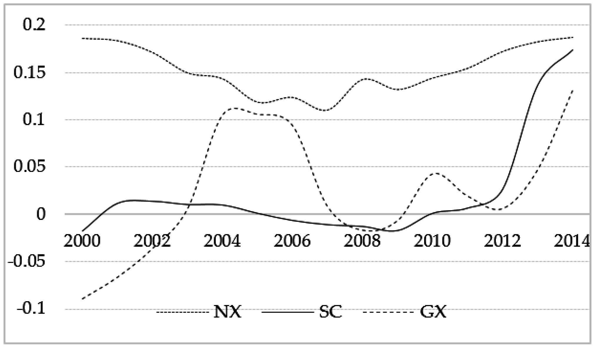
As we can observe in Figure 5, in Ningxia, LFIR had a relatively stable and positive effect on the coal supply ratio, with elastic coefficients ranging from 0.11 to 0.187. Given that in Ningxia, the ratio of added value in the financial industry remained high for several years, the response coefficients to the coal supply proportion changed with it, and, in consequence, fluctuated slightly. However, with 2007 as a turning point, the elastic coefficients gradually declined from 2000 to 2007 and arose from 2007 to 2014.
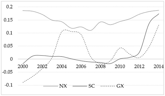
Figure 5.
The time-varying elastic coefficients of LFIR in NX, SC, and GX.
We can interpret this phenomenon by means of the “accumulative effect”. It is known to us that the ratio of added value in financial industry in Ningxia changed slightly during these years. However, the absolute added value in finance between 2000 and 2007 was on average 29.675, but averaged 139.481 between 2007 and 2014, nearly five times higher than the former. Therefore, the financial development level from 2000 to 2007 is lower, so the motivating effect of the ratio of added value in the financial sector has not been effectively exerted. According to the accumulative effect, this is demonstrated by the rapid financial development between 2007 and 2014.
In Sichuan, the impact of the added value in the financial industry (%GDP) on the coal supply ratio is relatively stable (before 2012) but alternates between positive and negative elastic coefficients. The elastic coefficient in 2000 was −0.018, which then decreased from 0.011 to 0.001 by 2005, and afterwards decreased to −0.017 by 2009. Finally, the elastic coefficient became positive again and reached 0.174 after a leap. Obviously, it is somewhat difficult to discuss the economic implications in contrast to Ningxia.
In order to give a reasonable interpretation, we try to combine the economic and financial policies for a specific year. In Sichuan, which benefited from the deepening of the financial revolution, the total assets in the banking sector broke 1 trillion by 2005. Together with the “develop-the-west” strategy and the “big industries” strategy, the coal industry was listed as one of the key development objectives, and experienced fast development within this period. The elastic coefficients within 2006–2009 are negative, indicating that financial development hindered coal production. From 2006, on the one hand, the Sichuan government made more investment into the electronic information and technology industry. The investment in electronic information and technology was 6.03 billion yuan, an increase of 69.9%. On the other hand, the local government put forward energy-saving and consumption-reducing regulations, such that the investment in coal industry was 12.8% lower than the previous year. Furthermore, together with the financial crisis in 2008 and the vigorous expansion of natural gas production, the coal production was suppressed. The elastic coefficients within 2010–2014 are positive, and start to jump from 2012. In fact, the ratio of the added value in financial industries during this period experienced tremendous growth, and broke 5% in 2012 (as seen in Figure 4). Why would the higher level of financial progress promote coal production? As we all know, the 2008 Wenchuan earthquake and 2013 Ya’an earthquake caused great damage to buildings. Therefore, it is deduced that a vast amount of cement and steel was needed to go towards post-disaster reconstruction, so more coal was necessary.
In Guangxi, the elastic coefficients of the ratio of added value in the financial industry to GDP on coal supply experience wide volatility, and alternate between positive and negative response coefficients. The elastic coefficients within 2000–2002 are negative, ranging from −0.09 to −0.067. From 2003 to 2007, the effect turns positive (0.006–0.106), and after experiencing an inverted “U” rollercoaster, the estimated coefficients abruptly turn negative in 2007–2008. From 2009 to 2014, the impact of the added value in financial industry to GDP on coal supply ratio remained positive; even so, the elastic coefficients were still volatile. Generally speaking, the ratio of coal supply in Guangxi is greatly influenced by the level of financial development.
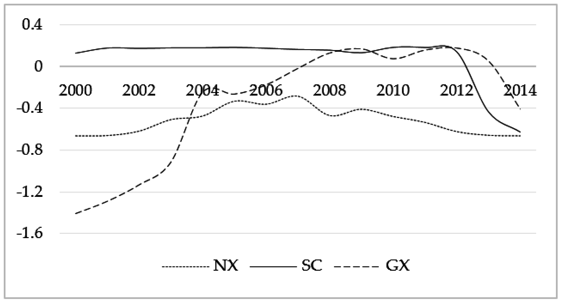
As seen in Figure 6, the elastic coefficients of the ratio of financial institutions’ loan balance (%GDP) (LLAN) to coal supply in Ningxia remain negative, ranging from –0.66 to –0.28, indicating that an increase of LLAN will help reduce the coal supply ratio. In addition, we also find it worth considering that the tendency of elastic coefficients in Figure 6 for Ningxia is opposite to that in Figure 5. Both of them take on a “U” shape, and both achieve the peak value in 2007. As mentioned early, the added value in financial industry (%GDP) ranges from 5% to 8%, standing for the higher development degree in the financial sector. Thus, we think that the increase of financial institutions’ loan balance (%GDP) will help reduce the coal supply ratio in Ningxia. Before 2007, this effect was becoming smaller and smaller. It can be interpreted according to the rule of “diminishing marginal utility”. Then, with the great technological investment during the period of financial crisis, the depression effect was gradually augmented.

Figure 6.
The time-varying elastic coefficients of LLAN in NX, SC, and GX.
In Sichuan, the elastic coefficients between 2000 and 2012 were kept around 0.2, implying that a 1% increase in the ratio of loan balance in financial institutions will make the coal supply ratio increase by 0.2%. However, the coefficients abruptly turned negative in 2013. As presented in Figure 6, the influence coefficient in 2013 was −0.435, and −0.66 in 2014. The main reason is that, from 2012, the problem of energy structure adjustment and environmental issues made the coal demand decrease. In this context, Sichuan province carried out a technical innovation project and closed down backward mines, such that the coal availability decreased.
In Guangxi, the variation of elastic coefficients is a bit complicated. From 2000 to 2007, the negative effect was generally reduced and specifically took on a “U” shape. From 2008 to 2013, the impact of the ratio of loan balance in financial institutions on the coal supply ratio became positive and had its minimum value in 2010. Then the influence direction became negative in 2014, with an elastic coefficient of −0.405.
In Figure 7, we find that the elastic coefficients between foreign direct investment actually utilized/GDP (LFDI) and coal supply ratio are constantly negative in Ningxia and Sichuan. In Ningxia, the coefficient variation is pretty steady, with a range from −0.166 to −0.131. In Sichuan, the elastic coefficients change from −0.155 to −0.038. In Guangxi, the influence factors from 2000 to 2003 are positive, and then abruptly turn negative. The FDI, on the one hand, benefits from the host country’s economic development, and accretes the coal consumption in energy production provinces; on the other hand, it makes for the improvement of the utilization efficiency of coal by technological innovation.

Figure 7.
The time-varying elastic coefficients of LFDI in NX, SC, and GX.
5.2. The Time-Varying Elasticity Analysis of the LTPG Specification
The thermal power generation proportion (LTPG) specification is a two-regime PSTR model with the ratio of investment in the coal mining and washing industry (LCIR) as the threshold variable. It denotes that LCIR is an influential factor leading to the nonlinear relationship in LTPG specification. The location parameter estimated in Table 5 is −4.724, located within the change interval for the value of the transition variable, and the transition rate is 1.84. We calculate the exponential location parameter 0.0089(e−4.724 = 0.0089). When LCIR is higher than 0.0089, the model gradually moves towards a high regime state as the threshold variable increases. Otherwise, the model gradually falls towards a low regime state as the threshold variable is reduced. In the observation of 255 LCIR series, only 15 of them were smaller than the position parameter: Guangxi (2000–2003), Hubei (1999–2004), Qinghai (2000–2002, 2004), and Jiangsu (2013) accounted for 5.9% of the whole interval range. This feature can also be seen in Figure 2, which shows the transition function for LTPG specification. The intensive degree of the values of transition functions on the right of the location parameter is significantly higher than that on the left side, meaning that most observed values are above the position parameter. Thus, the thermal power generation proportion (LTPG) specification is mainly located in the high regime.
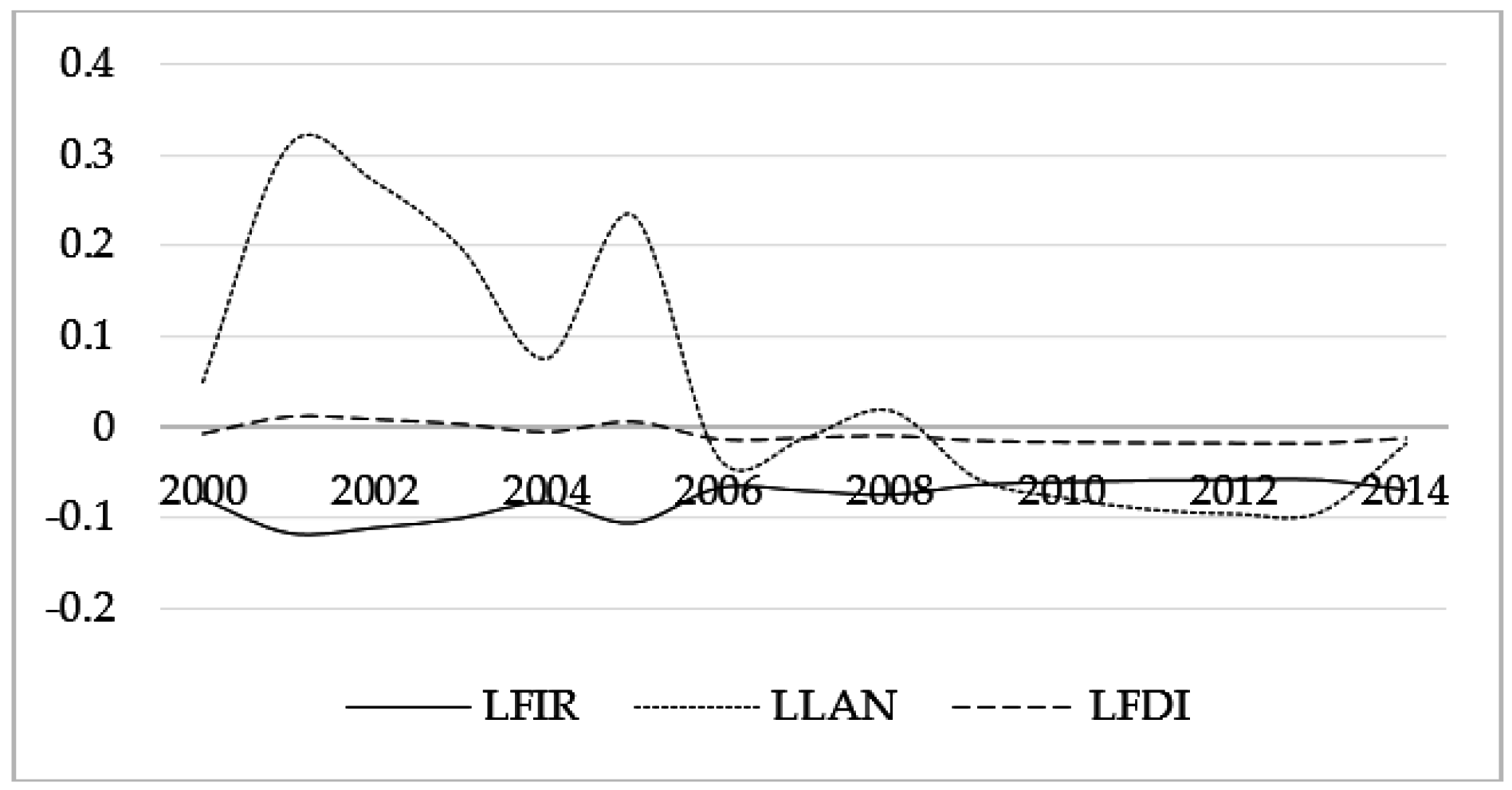
The impact of the added value in the financial industry (%GDP) on the thermal power generation proportion (LTPG) presents great volatility. In Table 5, the elastic coefficients are negative and the t-statistics are significant at the 95% confidence level, so the estimated coefficients are made up of linear and nonlinear parts, that is, . Because the transition function is between 0 and 1, the impact is negative and lower than –0.051. This means that there is a significant negative correlation relationship between the financial correlation ratio (LFIR) and the thermal power generation proportion (LTGP). It can also be observed from Figure 8 that the time-varying elasticity coefficients for LFIR are constantly negative, ranging from –0.117 to –0.066. In addition, the empirical results demonstrate that the individual time-varying elasticity coefficients for each province are also negative. This indicates that the increase in the financial correlation ratio (LFIR) in a country or region may contribute to a decrease in the thermal power generation proportion (LTPG).
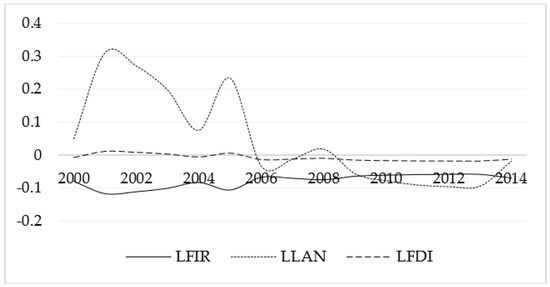
Figure 8.
Time-varying elasticity between financial development indicators and LTPG.
The estimation coefficient for the financial institutions’ loan balance/GDP (LLAN) is positive in the low regime, with an elasticity coefficient of 1.833, indicating that when the LLAN increases by 1%, the thermal power generation proportion (LTPG) will increase by 1.833% on average. In a high regime, the elasticity coefficient tends to be –0.131, indicating that when the LLAN increases by 1%, the thermal power generation proportion (LTPG) will decrease by 0.131% on average. To identify the turning point from positive to negative in the elasticity coefficient, we convert the transition function to obtain a turning point of 0.0374. This shows that when the investment in the coal mining and washing industry (LCIR) is larger than 3.74%, the correlation between LLAN and LTPG is negative. It can be concluded from Figure 8 that the elasticity coefficients between the financial institutions loan balance proportion (LLAN) and the thermal power generation proportion (LTPG) are first positive and then negative. Before the financial crisis of 2008, the coal industry was in a rapid development stage with strong market demand, so the expansion of the credit market promoted a thermal power generation increase. After the financial crisis in 2008, shocked by the slump of international energy price and the weak increase in the domestic economy, the market had less demand for coal and the corresponding sector. Thus, there was excess coal and thermal power generation production capacity at that time. In addition, with the gradual maturation of technology for nuclear, wind, and solar power generation, a “crowding-out effect” in the clean energy power generation market gradually became apparent, such that there was a negative correlation between the thermal power generation proportion and the loan balance.
Similarly, the elastic coefficient for foreign direct investment/GDP (LFDI) was positive in the linear part (low regime), with an elasticity coefficient of 0.122, indicating that when an 1% increase in financial openness increases, the thermal power generation proportion (LTPG) will increase by 0.122% on average. The elasticity coefficients in the high regime tend to be −0.021. By converting the transition function equation, we got the positive–negative turning point for the elasticity coefficients. When LCIR is smaller than 0.0234, the correlation relationship between financial openness (LFDI) and the thermal power generation proportion (LTPG) is positive; otherwise, the correlation relationship is negative. Of the 255 LCIR observed values, 27 of them are smaller than 0.023, accounting for about 14.5%. This indicates that there are mainly negative correlations between financial openness (LFDI) and the thermal power generation proportion (as shown in Figure 8), which was significant at a 95% confidence level. The reason for this negative correlation effect is that foreign direct investment in the energy sector in China significantly increased energy efficiency. Mielnika and Goldemberg (2002) examined the relationship between FDI and energy intensity in 20 developing countries, and concluded that it was the “spillover effect” of FDI technologies causing the progress in energy efficiency [41]. Therefore, an increase in the degree of financial openness could enhance energy utilization efficiency, thereby increasing the nuclear and wind power generation proportion because of their low energy intensity, and decreasing the thermal power generation proportion. In this model, the estimated coefficients for the control variable the investment in coal mining and processing industry (LCIR) are not significant. As this paper aims to explore the influence of the degree of financial development on energy supply structures, the impact of LCIR on LTPG is not analyzed here.
Due to space limitations, it is impossible to analyze the time-varying elasticity for all the individual provinces, so we just report on several representative provinces. In terms of LCSR specifications, we have discussed the time-varying effect of Ningxia, Sichuan, and Guangxi. In the LTPG model, the threshold value of LCIRit-1 = 0.89% divides the model into a linear part (low regime) and a nonlinear part (high regime). Figure 2 shows that values of transition function smaller than the threshold value 0.89% were observed in Guangxi (2000–2003), Hubei (1999–2004), Qinghai (2000–2002, 2004), and Jiangsu (2003). This denotes that the elasticity coefficients in the corresponding provinces and years are in the low regime, while the others tend towards the high regime. In order to identify the transition characteristics, in Table 6 we present the individual time-varying elasticity coefficients and make a simple analysis for the four provinces (Guangxi, Hubei, Qinghai, and Jiangsu).
Table 6.
Time-varying individual elasticities in LTPG specification.
6. Conclusions and Recommendations
This study investigated the threshold effect of financial development on the ratio of coal supply (LCSR) and the thermal power generation proportion (LTPG). LCSR specification is verified to be a four-regime PSTR model with the added value in financial industry/GDP (LFIR) as the transition variable, and the thermal power generation proportion (LTPG) specification is seen to be a two-regime model with the investment in the coal industry (LCIR) as the transition variable. Based on the empirical process and economic discussion, the following conclusions can be made.
- (1)
- Improving the ratio of the financial industry to GDP is helpful for hindering the overproduction of thermal power generation by 0.066%~0.117%. However, it is not helpful for the decrease of the ratio of coal production in high financial development regions such as Ningxia. Therefore, the financial sector can play a useful role in resolving the coal overcapacity. As is emphasized by numerous experts, finances play a dominant role in the process of supply-side reform, so the local government should make great effort to develop the financial industry in the future, which will be very helpful in reducing the coal overcapacity.
- (2)
- The impact of loans in financial institution/GDP on the ratio of coal supply is negative in high financial development regions such as Ningxia. In middle financial development region like Sichuan, the influence is mainly negative. In Guangxi, with the development of the financial industry, the impact is first positive and then negative. The impact on thermal power generation is also first positive and then negative with the increase of investment in the coal industry. Therefore, for the region with developed finances, the bank lending more money to energy enterprises is beneficial for resolving the problems of coal overcapacity, but in low financial development regions, banks should not give credit to debased businesses. For the local government, more investment in the coal industry will result in a decrease of thermal power generation.
- (3)
- The impact of foreign direct investment/GDP on the ratio of coal supply remained negative, ranging from−0.2 to −0.1. However, its influence on thermal power generation is negligible. In the past few decades, some local governments have been actively introducing FDI to promote economic development, such that local energy businesses can learn about advanced technology and management skills and improve energy efficiency. Meanwhile, they can also optimize their energy supply structure.
Against the backdrop of the “new normal” economy, how to maintain a balance between steady economic growth and structural adjustments to the energy supply is a tough problem. Financial development will play a critical role in boosting energy supply becoming more environmentally sustainable. Therefore, in the process of formulating energy conservation policies and related policies on energy supply and consumption, the government should consider transmission mechanisms via financial markets. This paper has some limitations, for example, in data availability: the data pool is somewhat small, which may adversely affect the precision of the empirical results. What is more, the financial indicators are not that comprehensive and there is a lack of stock market indexes. In the next stage, the authors will continue examining the relationship between financial development and energy supply (consumption) using a panel of country datasets.
Acknowledgments
This paper is supported by the National Natural Science Foundation of China (NSFC) under grant No. 71473155; the Young Star of Science and Technology plan project of China‘s Shaanxi province No. 2016KJXX-14; the China Postdoctoral Science Foundation under grant No. 2014T70130 . The authors would like to thank the anonymous referees as well as the editors.
Author Contributions
Jian Chai conceived and designed the experiments; Quanying Lu and Ting Liang collected and analyzed the data; Kin Keung Lai and Shouyang Wang contributed analysis tools and empirical analysis; Limin Xing performed the models and write the paper.
Conflicts of Interest
The authors declare no conflict of interest.
References
- National Bureau of Statistics of China (NBSC). China Statistical Yearbook 2016; China Statistics Press: Beijing, China, 2016.
- National Bureau of Statistics of China (NBSC). China Statistical Yearbook 2015; China Statistics Press: Beijing, China, 2015.
- The People’s Bank of China; National Development and Reform Commission; Ministry of Industry and Information; Ministry of Finance; Ministry of Commerce; China Banking Regulatory Commission; China Securities Regulatory Commission; China Insurance Regulatory Commission. Opinions on Financial Support for Industrial Steady Growth, Restructuring and Increasing Benefits [EB//OL]. Available online: http://www.pbc.gov.cn/goutongjiaoliu/113456/113469/3017867/index.html (accessed on 16 February 2016).
- Levine, R. Finance and Growth: Theory and Evidence; NBER Working Paper, No. 10766; Elsevier: Amsterdam, The Netherlands, 2004. [Google Scholar]
- Goldsmith, R.W. Financial Structure and Development; Yale University Press: New Haven, CT, USA, 1969. [Google Scholar]
- King, R.G.; Levine, R. Finance, entrepreneurship and growth: Theory and evidence. J. Monet. Econ. 1993, 32, 513–542. [Google Scholar] [CrossRef]
- Levine, R.; Zervos, S. Stock markets, banks, and economic growth. Am. Econ. Rev. 1998, 88, 537–558. [Google Scholar]
- Levine, R.; Zervos, S. Capital control liberalization and stock market development. World Dev. 1998, 26, 1169–1183. [Google Scholar] [CrossRef]
- Sadorsky, P. The impact of financial development on energy consumption in emerging economies. Energy Policy 2010, 38, 2528–2535. [Google Scholar] [CrossRef]
- Sadorsky, P. Financial development and energy consumption in Central and Eastern European frontier economies. Energy Policy 2011, 39, 999–1006. [Google Scholar] [CrossRef]
- Islam, F.; Shahbaz, M.; Ahmed, A.U.; Alam, M.M. Financial development and energy consumption nexus in Malaysia: A multivariate time series analysis. Econ. Model. 2013, 30, 435–441. [Google Scholar] [CrossRef]
- Zeren, F.; Koc, M. The nexus between energy consumption and financial development with asymmetric causality test: New evidence from newly industrialized countries. Int. J. Energy Econ. Policy 2014, 4, 83–91. [Google Scholar]
- Furuoka, F. Financial development and energy consumption: Evidence from a heterogeneous panel of Asian countries. Renew. Sustain. Energy Rev. 2015, 52, 430–444. [Google Scholar] [CrossRef]
- Lau, E.; Tan, C.C. Econometric analysis of the causality between energy supply and GDP: The case of Malaysia. Energy Procedia 2014, 61, 203–206. [Google Scholar] [CrossRef]
- Wang, B.Z.; Huang, J.Y. Relationship between energy supply, energy consumption and economic growth: Emprical study based on data on Shanxi province from 1978 to 2008. Technol. Econ. 2010, 2, 74–80. (In Chinese) [Google Scholar]
- Deidda, L.; Fattouh, B. Non-linearity between finance and growth. Econo. Lett. 2002, 74, 339–345. [Google Scholar] [CrossRef]
- Jude, E.C. Financial development and growth: A panel smooth regression approach. J. Econ. Dev. 2010, 35, 15–33. [Google Scholar]
- Doumbia, D. Financial development and economic growth in 43 advanced and developing economies over the period 1975–2009: Evidence of non-linearity. Appl. Econom. Int. Dev. 2016, 16, 13–22. [Google Scholar]
- Chang, S.C. Effects of financial developments and income on energy consumption. Int. Rev. Econ. Financ. 2015, 35, 28–44. [Google Scholar] [CrossRef]
- Lee, C.C.; Chiu, Y.B. Electricity demand elasticities and temperature: Evidence from panel smooth transition regression with instrumental variable approach. Energy Econ. 2011, 33, 896–902. [Google Scholar] [CrossRef]
- Lee, C.C.; Chiu, Y.B. Modeling OECD energy demand: An international panel smooth transition error-correction model. Int. Rev. Econ. Financ. 2013, 25, 372–383. [Google Scholar] [CrossRef]
- Tamazian, A.; Chousa, J.P.; Vadlamannati, K.C. Does higher economic and financial development lead to environmental degradation: Evidence from BRIC countries? Energy Policy 2009, 37, 246–253. [Google Scholar] [CrossRef]
- Zhang, Y.J. The impact of financial development on carbon emissions: An empirical analysis in China. Energy Policy 2011, 39, 2197–2203. [Google Scholar] [CrossRef]
- González, A.; Teräsvirta, T.; Dijk, D. Panel Smooth Transition Regression Models; University of Technology Sydney: Sydney, Australia, 2005. [Google Scholar]
- Aslanidis, N.; Xepapadeas, A. Regime switching and the shape of the emission—Income relationship. Econ. Model. 2008, 25, 731–739. [Google Scholar] [CrossRef]
- National Bureau of Statistics of China. Available online: http://data.stats.gov.cn/easyquery.htm?cn=C01 (accessed on 10 October 2016). (In Chinese)
- The People’s Bank of China. Available online: http://www.pbc.gov.cn/rmyh/105223/105413/index.html (accessed on 10 October 2016). (In Chinese)
- Wind Economic Database. Available online: http://www.wind.com.cn/en/edb.html (accessed on 10 October 2016). (In Chinese)
- Batten, J.A.; Vo, X.V. An analysis of the relationship between foreign direct investment and economic growth. Appl. Econ. 2009, 41, 1621–1641. [Google Scholar] [CrossRef]
- Doytch, N.; Narayan, S. Does FDI influence renewable energy consumption? An analysis of sectoral FDI impact on renewable and non-renewable industrial energy consumption. Energy Econ. 2016, 54, 291–301. [Google Scholar] [CrossRef]
- Yuan, Y.J.; Guo, L.L.; Sun, J. Structure, technology, management and energy efficiency—Stochastic frontier approach based on provincial panel data during 2000–2010. China Ind. Econ. 2012, 7, 18–30. (In Chinese) [Google Scholar]
- Beck, T.; Démirguc-Kunt, A.; Levine, R. Financial Institutions and Markets across Countries and over Time-Data and Analysis; World Bank Group Publication: Washington, DC, USA, 2009. [Google Scholar]
- Sun, P.Y.; Wang, Y.N.; Cen, Y. Does financial development affect energy consumption structure? Exploring the global evidences. Nankai Econ. Stud. 2011, 2, 28–41. (In Chinese) [Google Scholar]
- Shen, M.; Shen, L.; Zhang, Y. The stability of Shaanxi’s energy supply system and its influencing factors. Econ. Geogr. 2015, 35, 39–46. (In Chinese) [Google Scholar]
- Granger, C.W.J.; Terasvirta, T. Modelling Non-Linear Economic Relationships; Oxford University Press: Oxford, UK, 1993. [Google Scholar]
- Teräsvirta, T. Specification, estimation, and evaluation of smooth transition autoregressive models. J. Am. Stat. Assoc. 1994, 89, 208–218. [Google Scholar]
- Van Dijk, D.; Teräsvirta, T.; Franses, P. Smooth transition autoregressive models: A survey of recent developments. Econom. Rev. 2002, 21, 1–47. [Google Scholar] [CrossRef]
- Davies, R.B. Hypothesis testing when a nuisance parameter is present only under the alternative. Biometrika 1977, 64, 247–254. [Google Scholar] [CrossRef]
- Colletaz, G.; Hurlin, C. Threshold Effects of the Public Capital Productivity: An International Panel Smooth Transition Approach; University of Orléans: Orléans, France, 2008. [Google Scholar]
- Fouquau, J.; Hurlin, C.; Rabaud, I. The Feldstein–Horioka puzzle: A panel smooth transition regression approach. Econ. Model. 2008, 25, 284–299. [Google Scholar] [CrossRef]
- Mielnik, O.; Goldemberg, J. Foreign direct investment and decoupling between energy and gross domestic product in developing countries. Energy Policy 2002, 30, 87–89. [Google Scholar] [CrossRef]


© 2016 by the authors; licensee MDPI, Basel, Switzerland. This article is an open access article distributed under the terms and conditions of the Creative Commons Attribution (CC-BY) license (http://creativecommons.org/licenses/by/4.0/).