
Energy and Greenhouse Gas Emission Assessment of Conventional and Solar Assisted Air Conditioning Systems


Abstract
:1. Introduction
2. Methodology
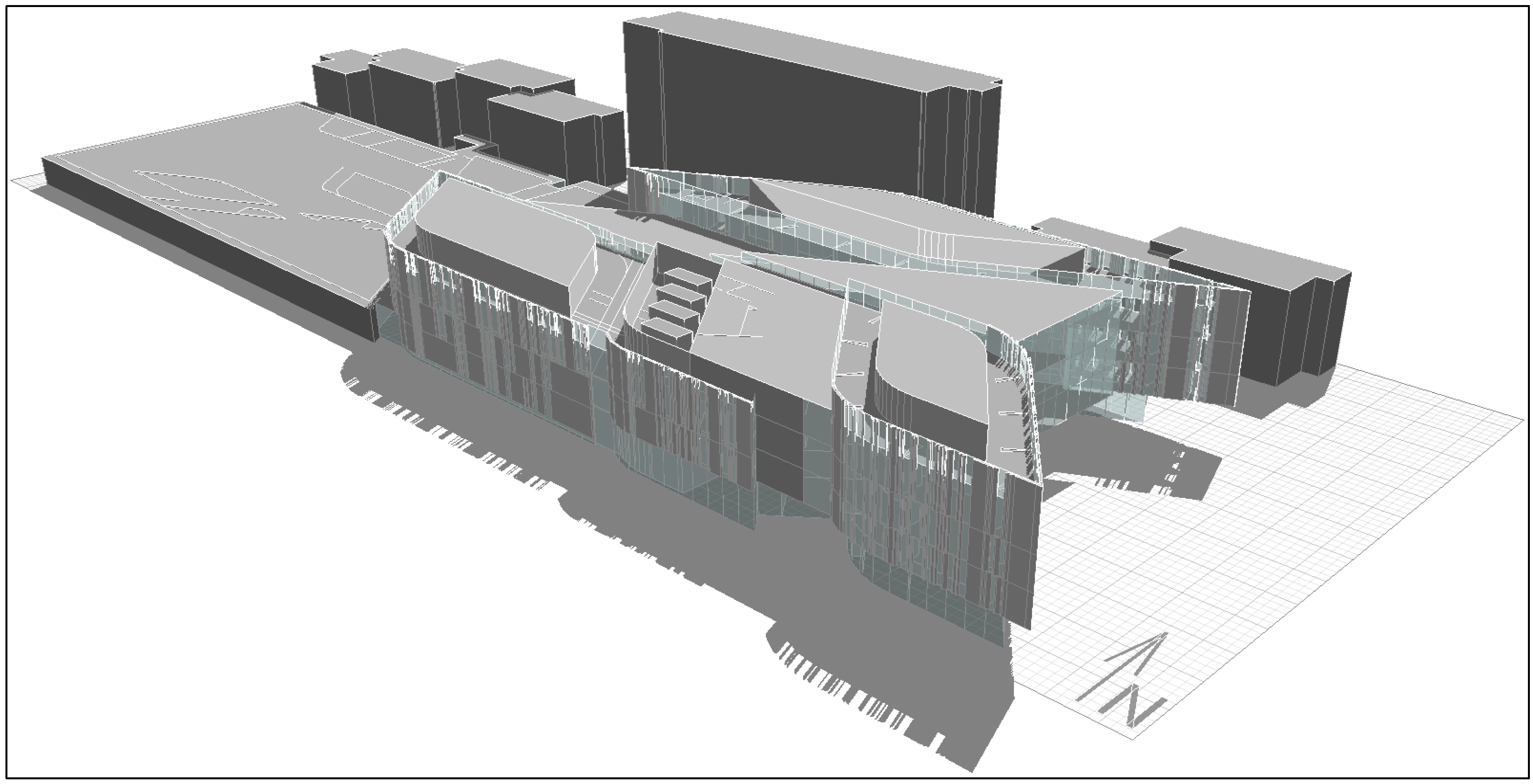
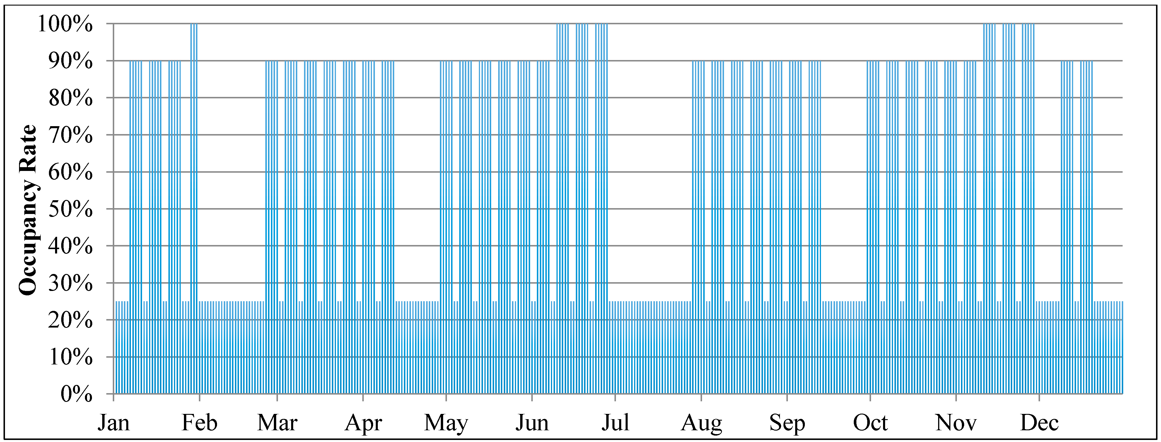
2.1. Building Description


| Constructions | R | U | VLT | SHGC |
|---|---|---|---|---|
| m2K/W | W/m2K | % | ||
| External wall (lower ground and ground level) | 1.78 | 0.56 | - | - |
| Roof (flat roof and metal roof) | 3.28 | 0.311 | - | - |
| Glazing (windows and curtain walls) | - | 1.69 | 62 | 0.29 |
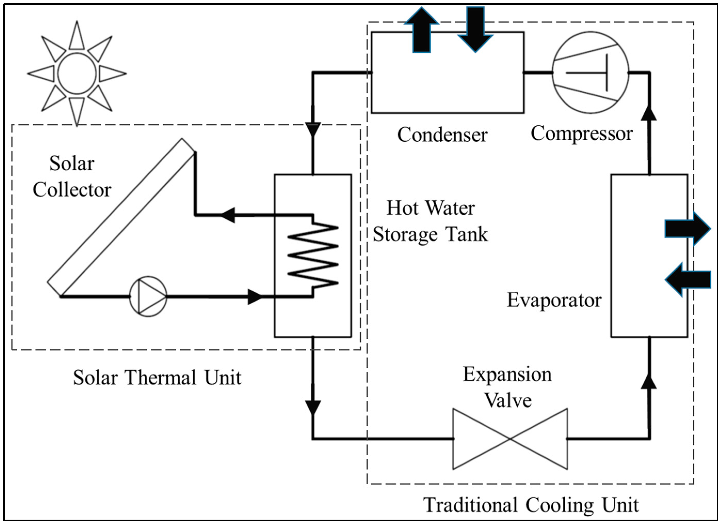
2.2. System Description
| Building | Cooling Method | Cooling Equipment | Energy Source | Scenario |
|---|---|---|---|---|
| Cooling Demand | Conventional System | Water Cooled Chiller (WCC) | Grid | 1 |
| PV | 2 | |||
| Air Cooled Chiller (ACC) | Grid | 3 | ||
| PV | 4 | |||
| Solar Assisted System | Hybrid Solar Air Conditioner (HSAC) | Grid + Solar Thermal | 5 | |
| PV + Solar Thermal | 6 |
2.3. Solar Simulation Description
2.4. Energy Simulation Description
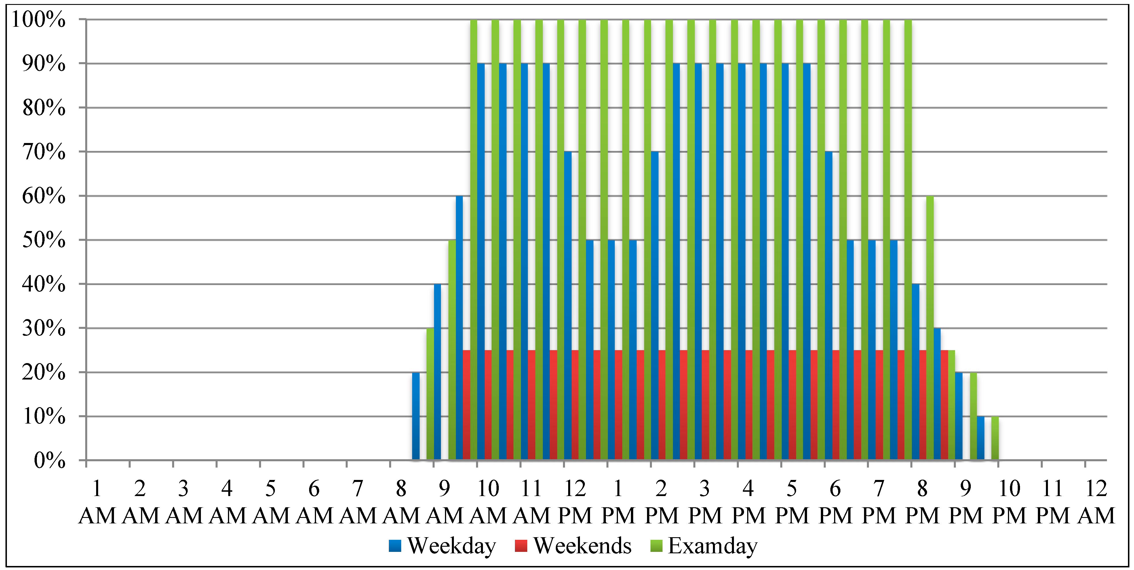
2.4.1. Cooling Demand Simulation
| Parameters | Units | Design value | |
|---|---|---|---|
| LGL, GL | L1, L2, L3 | ||
| People Density | people/m2 | 0.2 | 0.1 |
| Metabolic heat | W/person | 135 | 123 |
| Equipment heat | W/m2 | 5 | 15 |
| Lighting heat | W/m2 | 12 | 10 |
| Cooling set point | °C | 25 | 25 |
| Relative humidity | % | 60 | 60 |
| Ventilation/Infiltration | V/h | 0.3 | 0.3 |

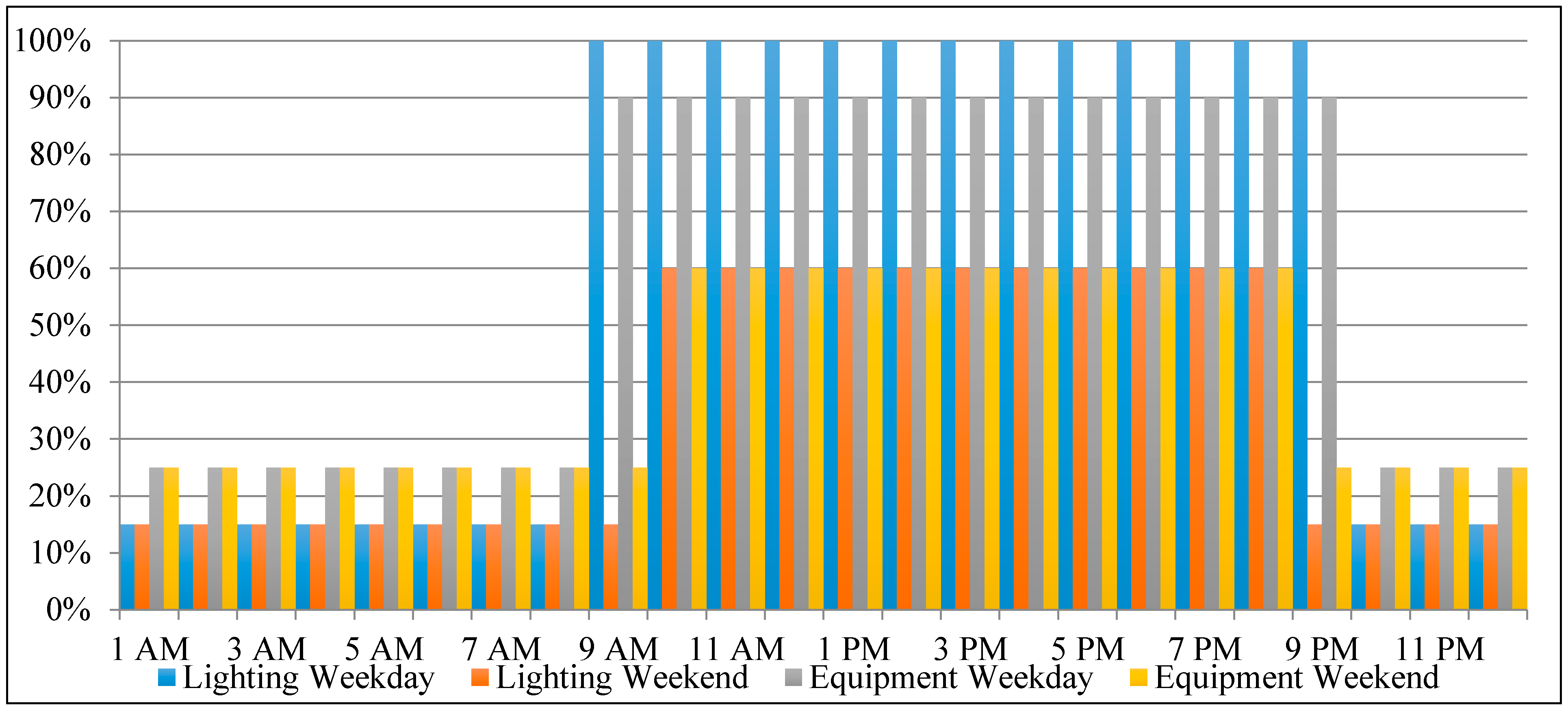
2.4.2. Energy Consumption Simulation
2.5. Greenhouse Gas Emission Prediction
| g CO2-e/kWh | |
|---|---|
| New South Wales electricity grid | 900 |
| Photovoltaic | 90 |
3. Results
3.1. Solar Energy Potential
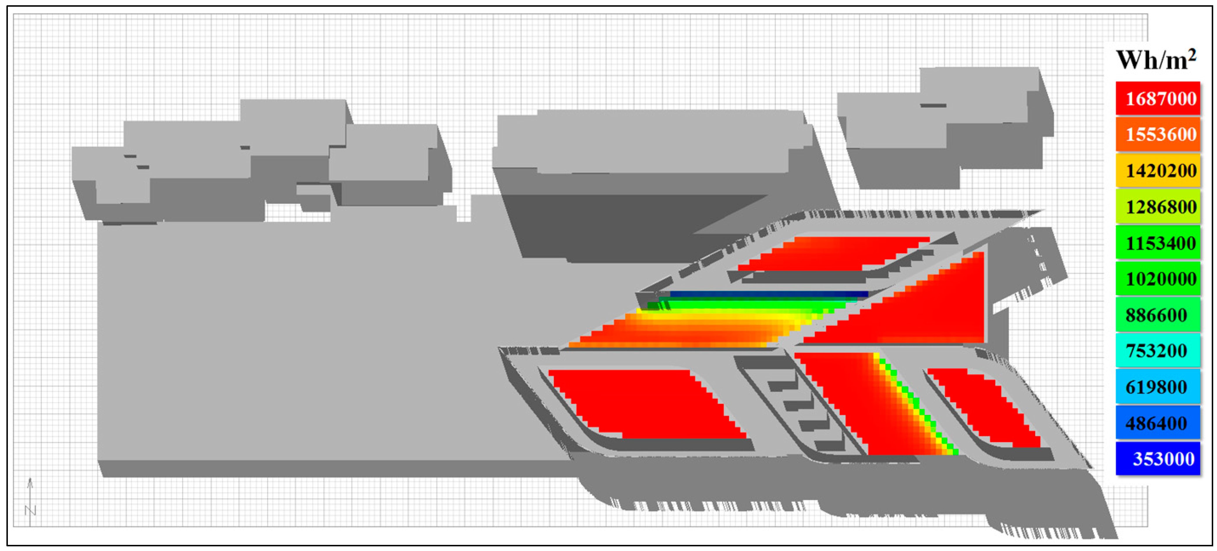
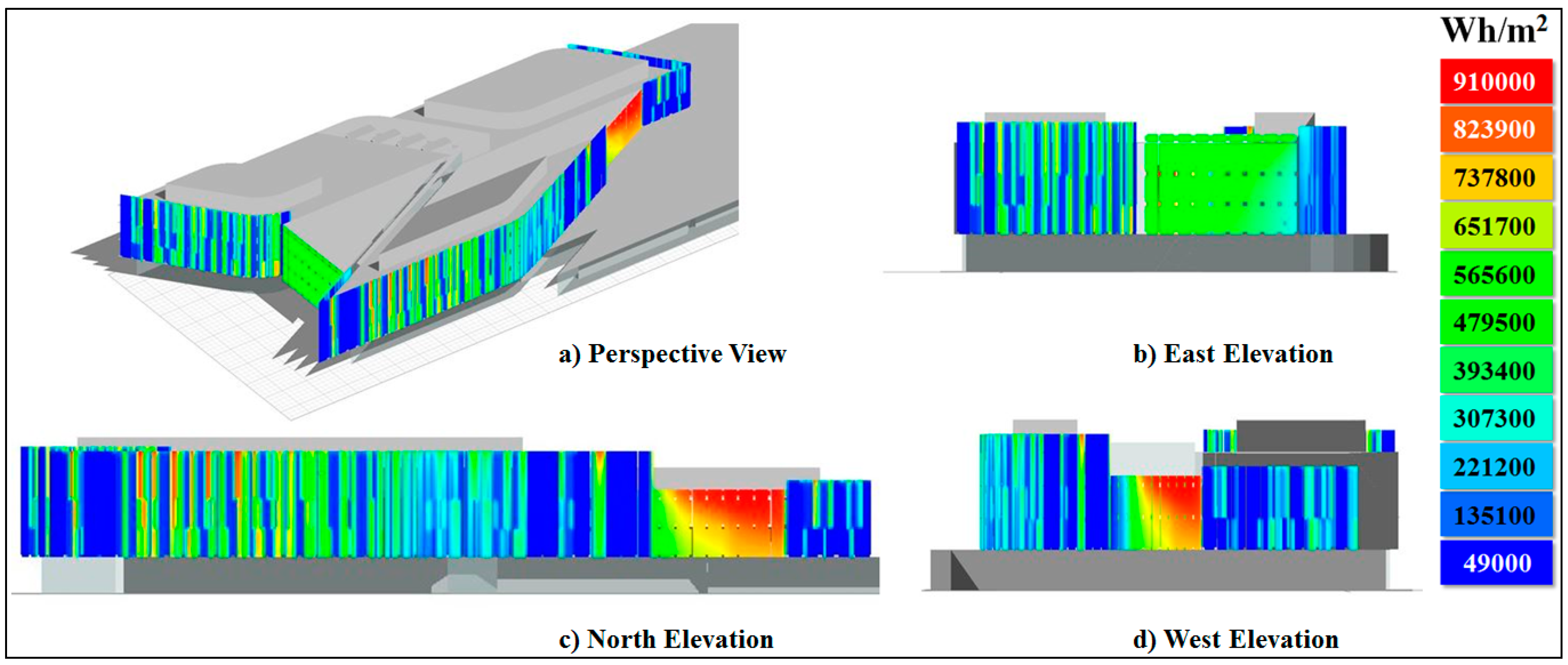
| Building Surfaces | PV Cell Types | Efficiency | Area of Panels a | Available Solar Radiation | Electric Power Generated b |
|---|---|---|---|---|---|
| m2 | MWh | MWh | |||
| Roof | Multicrystalline | 15% | 1474 (1374) | 2311.7 | 346.8 (323.3) |
| East side | Amorphous | 8% | 708 | 204.7 | 16.4 |
| North side | Amorphous | 8% | 609 | 174.9 | 14.0 |
| West side | Amorphous | 8% | 744 | 206.1 | 16.5 |
| SUM | 3535 (3435) | 2897.4 | 393.7 (370.2) |
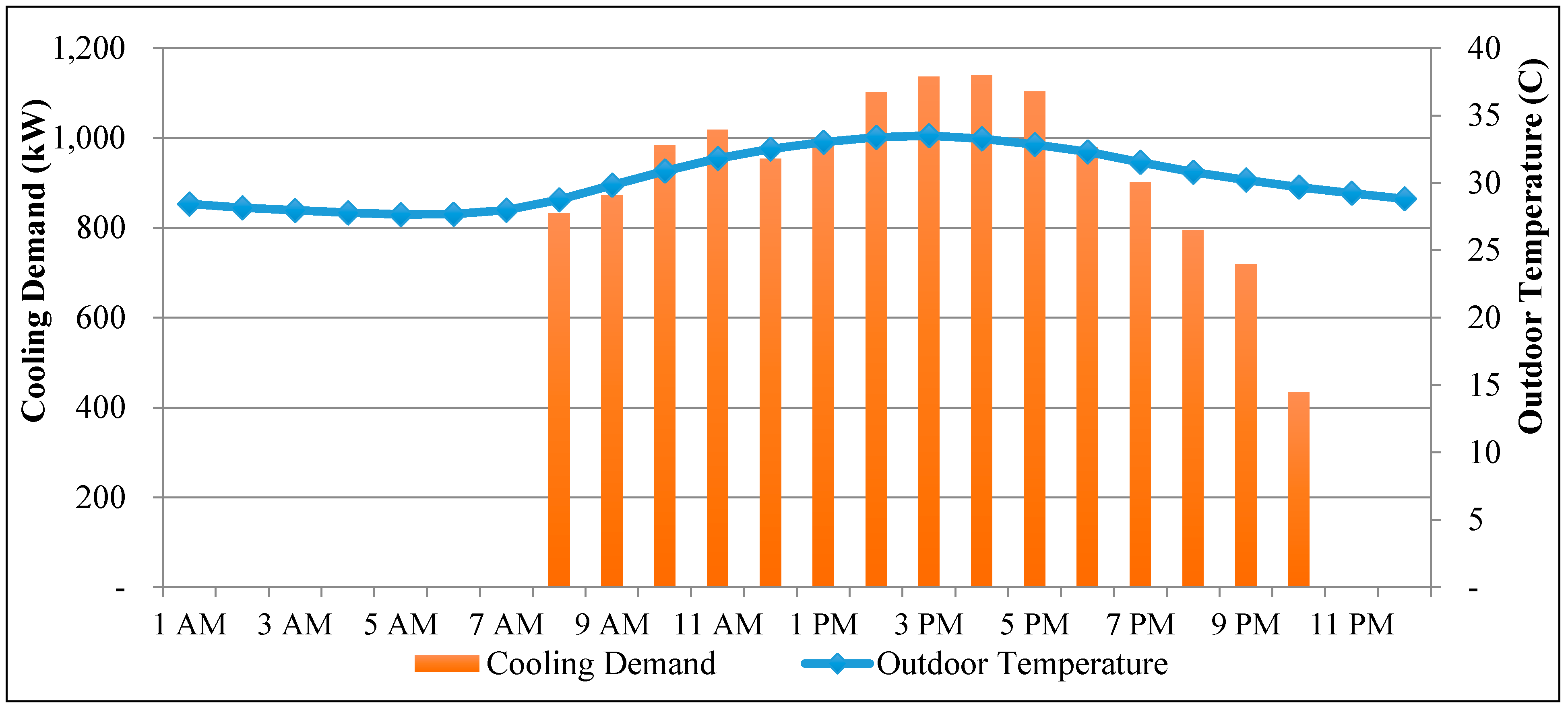
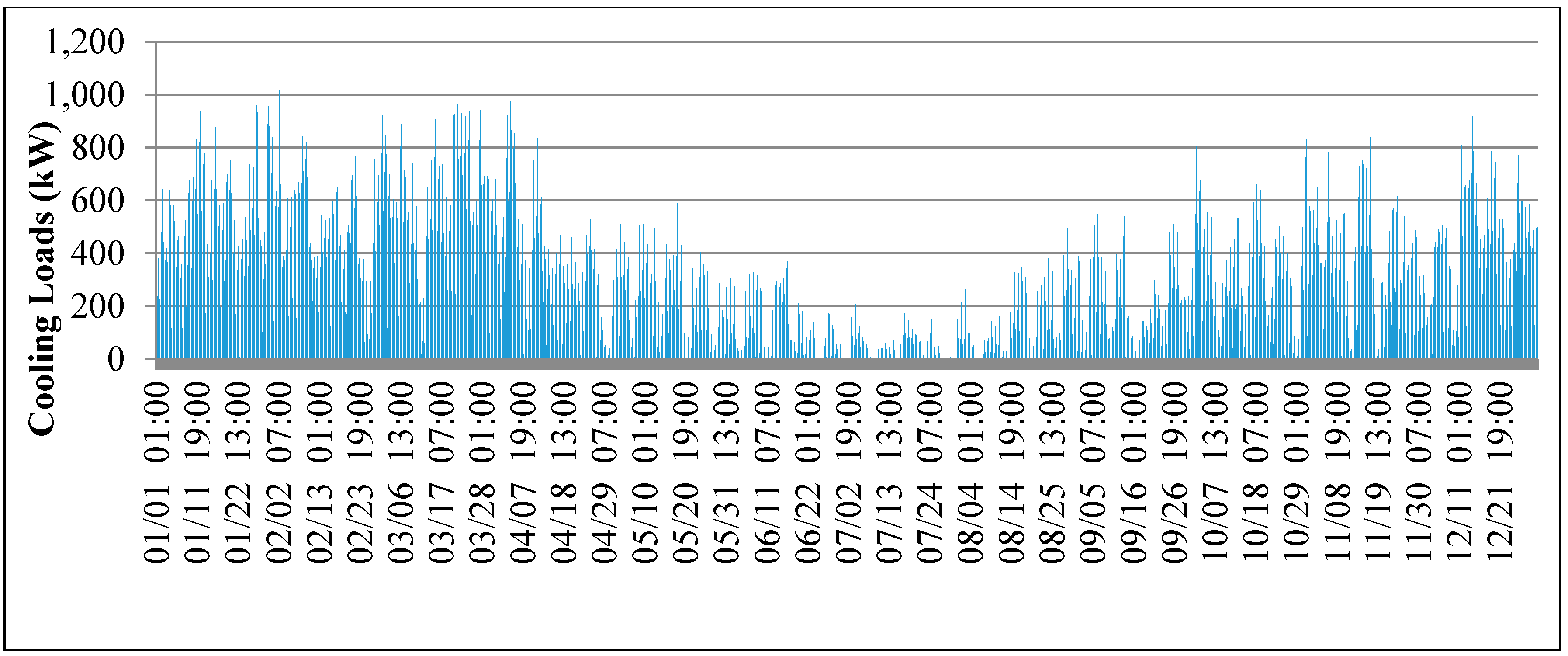
3.2. Cooling Demands of the Building

3.3. System Performance Comparisons

| Specifications | Water Cooled Chiller (WCC) | Air Cooled Chiller (ACC) |
|---|---|---|
| Capacity | 850.0 kW | 850.0 kW |
| Refrigerant | HFC 134a | HFC 134a |
| Compressors | Centrifugal | Centrifugal |
| Evaporator Entering Water Temperature | 14.5 °C | 14.5 °C |
| Evaporator Leaving Water Temperature | 4.0 °C | 4.0 °C |
| Condenser Entering Water Temperature | 28.0 °C | - |
| Condenser Leaving Water Temperature | 38.0 °C | - |
| Condenser Ambient Temperature | - | 35.0°C |
| Partial loads (%) | 100% | 75% | 50% | 25% |
| Cooling hours (h) | 487 | 985 | 1448 | 2060 |
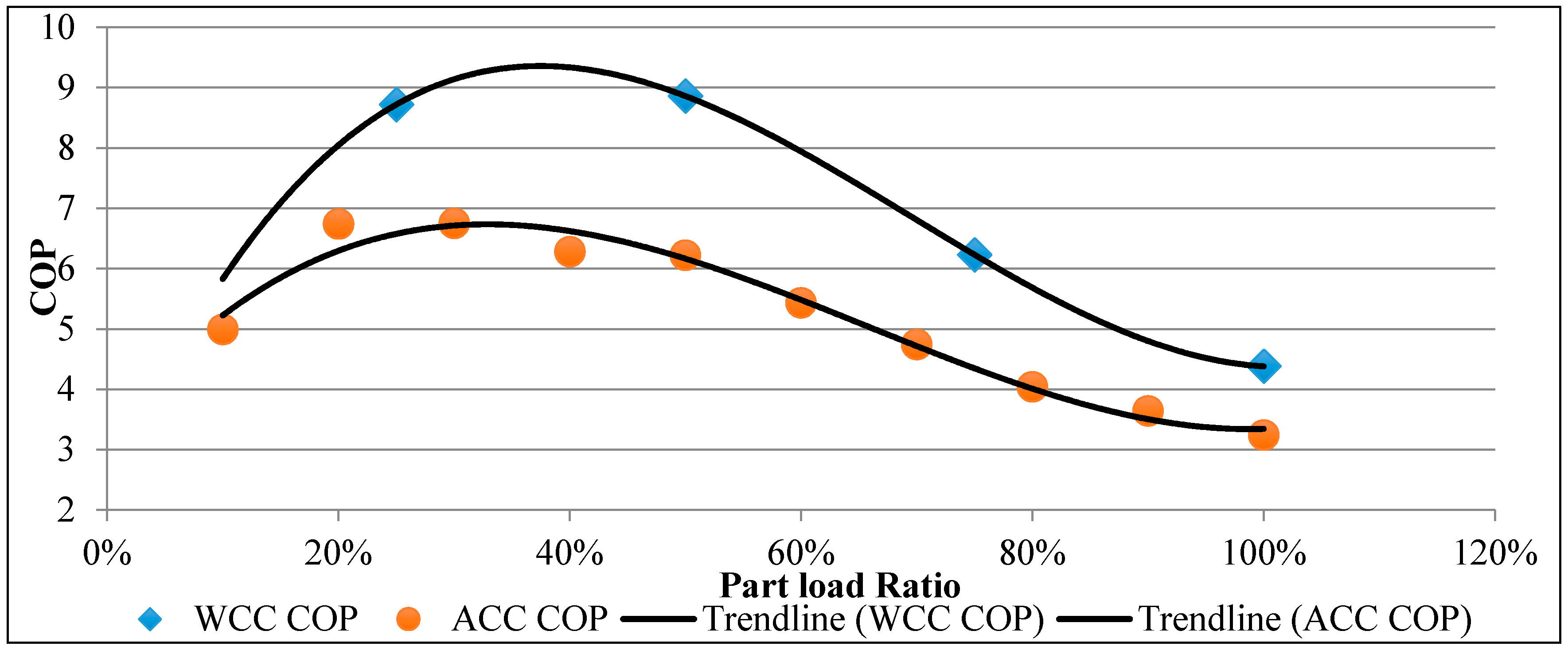
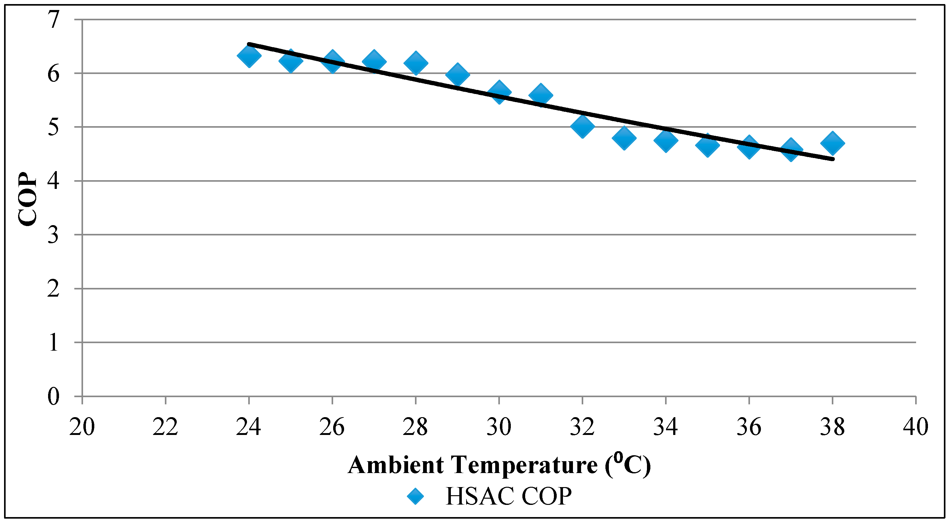
| Cooling Unit | a0 | a1 | a2 | a3 | R2 |
|---|---|---|---|---|---|
| WCC | 37.867 | −78.960 | 43.213 | 2.260 | 1.00 |
| ACC | 23.693 | −46.786 | 23.074 | 3.362 | 0.973 |
| HSAC | - | 0.001 | −0.227 | 11.295 | 0.914 |

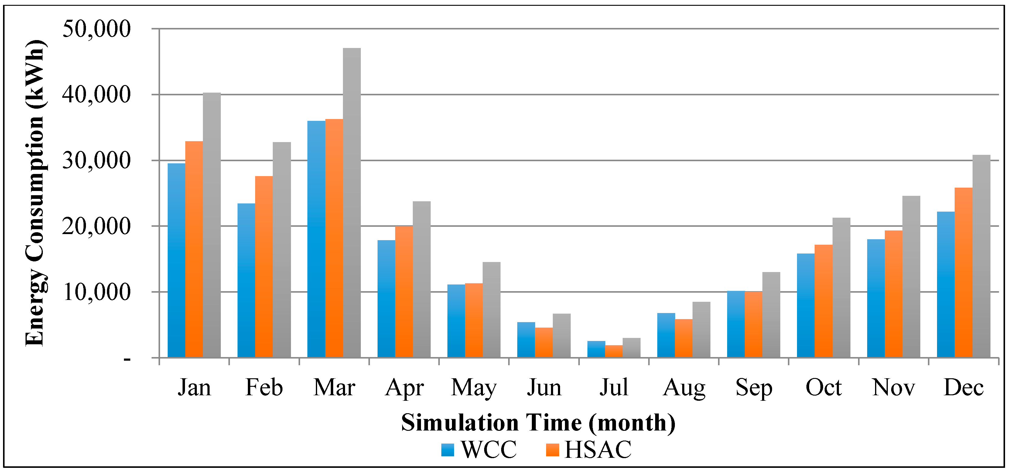
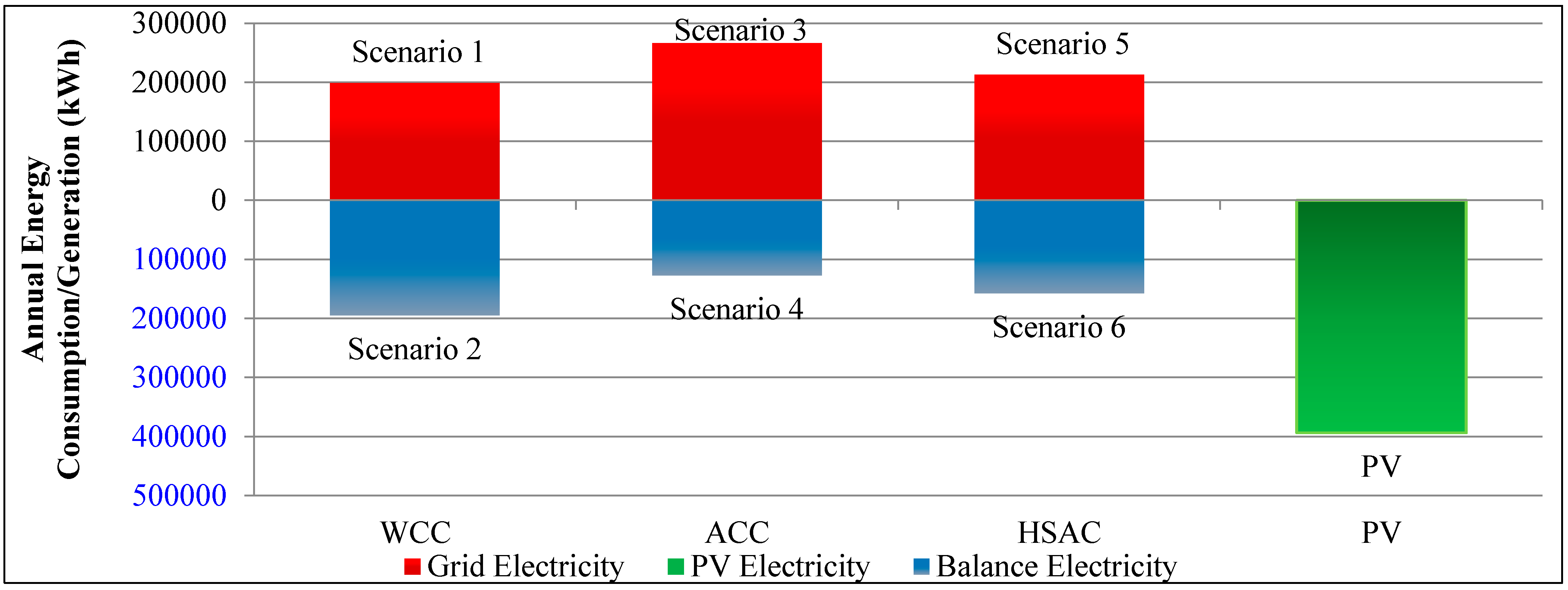
3.4. Energy Consumption and Energy Saving Potential
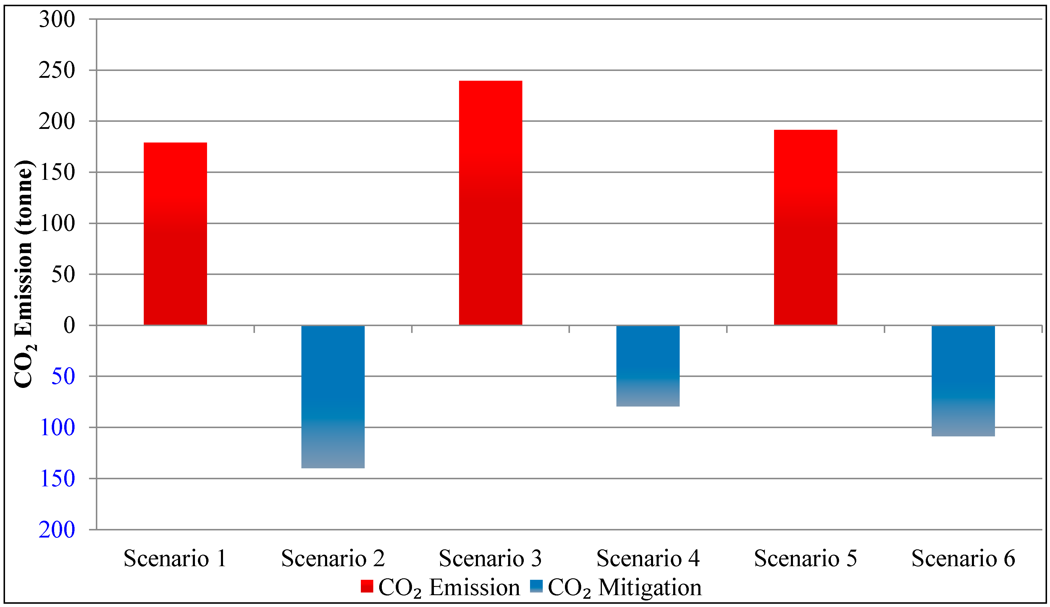
3.5. Greenhouse Gas Emission Comparison for Cooling Systems

4. Conclusions
- (1)
- The simulation results indicate that, under ideal conditions, if PV panels are installed on the investigated building, they will entirely cover for the annual electricity consumption for cooling of the building.
- (2)
- The overall performance of the Hybrid Solar Air Conditioner (HSAC) is higher than the Air Cooled Chiller (ACC) but lower than the Water Cooled Chiller (WCC).
- (3)
- The annual energy consumption of the HSAC was found to be lower than the ACC while it consumes more electricity than the WCC system. The BIPV technology can effectively reduce the electricity demand in the peak load period.
- (4)
- Additionally, the greenhouse gas emissions caused by cooling the building could be completely offset by the use of renewable energy. The surplus electricity could be also used by other electronic appliances in the building to further mitigate the greenhouse gas emissions when the solar based PV technology is integrated in the building.
Acknowledgments
Author Contributions
Conflicts of Interest
Abbreviations
| ACC | Air Cooled Chiller |
| BIPV | Building Integrated Photovoltaic |
| COP | Coefficient of Performance |
| GHG | Greenhouse Gas |
| GL | Ground Level |
| HSAC | Hybrid Solar Air Conditioner |
| LGL | Lower Ground Level |
| PV | Photovoltaic |
| R-value | Thermal Resistance Value |
| SHGC | Solar Heat Gain Coefficient |
| U-value | Overall Heat Transfer Co-Efficient |
| VLT | Visible Light Transmission |
| WCC | Water Cooled Chiller |
References
- Marini, D. Optimization of HVAC systems for distributed generation as a function of different types of heat sources and climatic conditions. Appl. Energy 2013, 102, 813–826. [Google Scholar] [CrossRef]
- Ascione, F.; Bianco, N.; de Masi, R.F.; Mauro, G.M.; Vanoli, G.P. Design of the building envelope: A novel multi-objective approach for the optimization of energy performance and thermal comfort. Sustainability 2015, 7, 10809–10836. [Google Scholar] [CrossRef]
- Henning, H.M. Solar assisted air conditioning of buildings––An overview. Appl. Therm. Eng. 2007, 27, 1734–1749. [Google Scholar] [CrossRef]
- Cheong, C.H.; Kim, T.; Leigh, S.B. Thermal and daylighting performance of energy-efficient windows in highly glazed residential buildings: Case study in Korea. Sustainability 2014, 6, 7311–7333. [Google Scholar] [CrossRef]
- Li, X.; Strezov, V.; Amati, M. A qualitative study of motivation and influences for academic green building developments in Australian universities. J. Green Build. 2013. [Google Scholar] [CrossRef]
- Todorovic, M.S. BS, energy efficiency and renewable energy sources for buildings greening and zero energy cities planning harmony and ethics of sustainability. Energy Build. 2012, 48, 180–189. [Google Scholar] [CrossRef]
- Australian Energy Resource Assessment. Available online: http://www.ga.gov.au/corporate_data/70142/70142_complete.pdf (accessed on 2 November 2015).
- Davy, R.J.; Troccoli, A. Interannual variability of solar energy generation in Australia. Sol. Energy 2012, 86, 3554–3560. [Google Scholar] [CrossRef]
- Kim, J.T.; Todorovic, M.S. Tuning control of buildings glazing’s transmittance dependence on the solar radiation wavelength to optimize daylighting and building’s energy efficiency. Energy Build. 2013, 63, 108–118. [Google Scholar] [CrossRef]
- Peng, C.H.; Huang, Y.; Wu, Z.S. Building-integrated photovoltaics (BIPV) in architectural design in China. Energy Build. 2011, 43, 3592–3598. [Google Scholar] [CrossRef]
- Miyazaki, T.; Akisawa, A.; Kashiwagi, T. Energy savings of office buildings by the use of semi-transparent solar cells for windows. Renew. Energy 2005, 30, 281–304. [Google Scholar] [CrossRef]
- Wong, P.W.; Shimoda, Y.; Nonaka, M.; Inoue, M.; Mizuno, M. Semi-transparent PV: Thermal performance, power generation, daylight modelling and energy saving potential in a residential application. Renew. Energy 2008, 33, 1024–1036. [Google Scholar] [CrossRef]
- Yu, M.; Halog, A. Solar photovoltaic development in australia––A life cycle sustainability assessment study. Sustainability 2015, 7, 1213–1247. [Google Scholar] [CrossRef]
- Enteria, N.; Yoshino, H.; Takaki, R.; Yonekura, H.; Satake, A.; Mochida, A. First and second law analyses of the developed solar-desiccant air-conditioning system (SDACS) operation during the summer day. Energy Build. 2013, 60, 239–251. [Google Scholar] [CrossRef]
- Zhai, X.Q.; Qu, M.; Li, Y.; Wang, R.Z. A review for research and new design options of solar absorption cooling systems. Renew. Sustain. Energy Rev. 2011, 15, 4416–4423. [Google Scholar] [CrossRef]
- Chemisana, D.; Lopez-Villada, J.; Coronas, A.; Rosell, J.I.; Lodi, C. Building integration of concentrating systems for solar cooling applications. Appl. Therm. Eng. 2013, 50, 1472–1479. [Google Scholar] [CrossRef]
- Ha, Q.P.; Vakiloroaya, V. A novel solar-assisted air-conditioner system for energy savings with performance enhancement. Procedia Eng. 2012, 49, 116–123. [Google Scholar] [CrossRef]
- Green Building Council of Australia. The Dollars and Sense of Green Buildings: Building the Business Case for Green Commercial Buildings in Australia; Green Building Council of Australia (GBCA): Sydney, Australia, 2008. [Google Scholar]
- Todorovic, M.S.; Kim, J.T. Buildings energy sustainability and health research via interdisciplinarity and harmony. Energy Build. 2012, 47, 12–18. [Google Scholar] [CrossRef]
- Ibarra, D.; Reinhart, C.F. Solar Availability: A Comparison Study of Six Irradiation Distribution Methods. In Proceedings of the Building Simulation: 12th Conference of International Building Performance Simulation Association, Sydney, Australia, 14–16 November 2011; pp. 2627–2634.
- Crawley, D.B.; Hand, J.W.; Kurnmert, M.; Griffith, B.T. Contrasting the capabilities of building energy performance simulation programs. Build. Environ. 2008, 43, 661–673. [Google Scholar] [CrossRef]
- DOE. About Energyplus. Available online: http://apps1.eere.energy.gov/buildings/energyplus/energyplus_about.cfm. (accessed on 30 April 2013).
- Pang, X.F.; Wetter, M.; Bhattacharya, P.; Haves, P. A framework for simulation-based real-time whole building performance assessment. Build. Environ. 2012, 54, 100–108. [Google Scholar] [CrossRef]
- Evans, A.; Strezov, V.; Evans, T.J. Assessment of sustainability indicators for renewable energy technologies. Renew. Sustain. Energy Rev. 2009, 13, 1082–1088. [Google Scholar] [CrossRef]
- National Greenhouse Accounts (NGA) Factors. Available online: https://www.environment.gov.au/system/files/resources/7326bc48-03d8-4e78-a57c-90e3ba85efe8/files/national-greenhouse-accounts-factors-july-2013.pdf (accessed on 2 November 2015).
- Whitman, B.; Johnson, B.; Tomczyk, J. Refrigeration and Air Conditioning Technology, 6th ed.; Delmar Cengage Learning: Clifton Park, NY, USA, 2009. [Google Scholar]
- Kim, J.H.; Kim, H.R.; Kim, J.T. Analysis of photovoltaic applications in zero energy building cases of IEA SHC/EBC task 40/annex 52. Sustainability 2015, 7, 8782–8800. [Google Scholar] [CrossRef]
© 2015 by the authors; licensee MDPI, Basel, Switzerland. This article is an open access article distributed under the terms and conditions of the Creative Commons Attribution license (http://creativecommons.org/licenses/by/4.0/).
Share and Cite
Li, X.; Strezov, V. Energy and Greenhouse Gas Emission Assessment of Conventional and Solar Assisted Air Conditioning Systems. Sustainability 2015, 7, 14710-14728. https://doi.org/10.3390/su71114710
Li X, Strezov V. Energy and Greenhouse Gas Emission Assessment of Conventional and Solar Assisted Air Conditioning Systems. Sustainability. 2015; 7(11):14710-14728. https://doi.org/10.3390/su71114710
Chicago/Turabian StyleLi, Xiaofeng, and Vladimir Strezov. 2015. "Energy and Greenhouse Gas Emission Assessment of Conventional and Solar Assisted Air Conditioning Systems" Sustainability 7, no. 11: 14710-14728. https://doi.org/10.3390/su71114710
APA StyleLi, X., & Strezov, V. (2015). Energy and Greenhouse Gas Emission Assessment of Conventional and Solar Assisted Air Conditioning Systems. Sustainability, 7(11), 14710-14728. https://doi.org/10.3390/su71114710