Developing a Cell-Based Spatial Optimization Model for Land-Use Patterns Planning


Abstract
:1. Introduction
2. Methods and Materials
2.1. Dynamically Dimensioned Search Land-Use Optimization Planning Tool (DDSLOP Tool)

- Define maximum iteration count tmax for outer fitness function evaluations.
- Define maximum iteration count imax for inner fitness function evaluations.
- Define initial solution of outer control variable (composition) and inner control variable (configuration) , which denotes the spatial composition and configuration, respectively, of the original-unmodified landscape. Where Mm,n represents the land-use type at location (m, n).
- Current best fitness .
- Current best solution and for outer and inner optimization, respectively.
- Calculate the proportion of land-use type ratios, which will be selected for modification, based on a function of current iteration count: .
- For d = 1, …, D, move pd from to {N} until j control variables have been selected, (j ˂ D) based on the .
- If {N} is empty, randomly place one element from into it.
- , where .
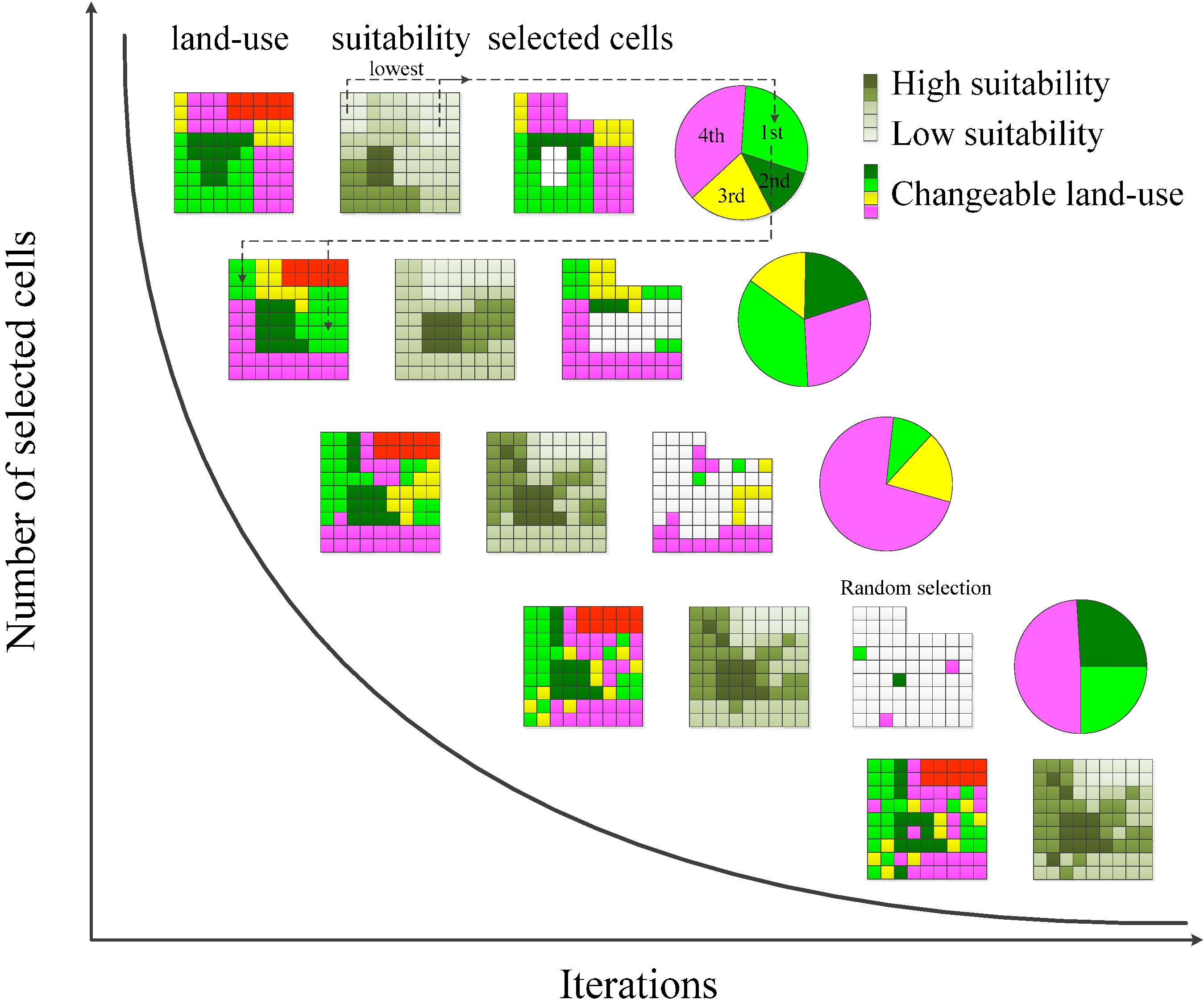
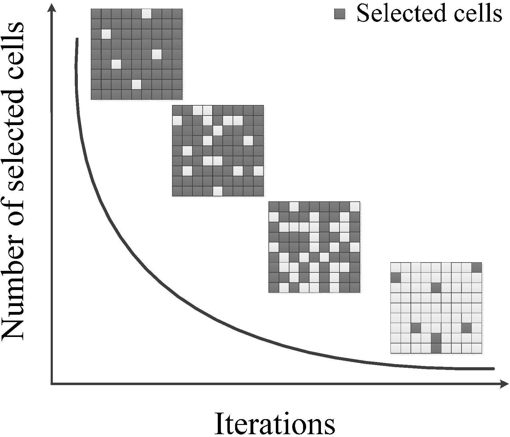
- Stochastically select k elements from (current best land use raster data set) and place these into a pool . For each iteration, the proportion of selected cells corresponds to the function of current iteration count .
- ■
- Rank selected cells in accordance to their relative hsi(Mx,y) at (x,y).
- ■
- Preferentially select cells in hsi(Mx,y) ascending order (lower values first) and place into , the proportion of selected cells for each iteration is equivalent to the function (Figure 2).
- Exchange the land-use type of each element in .
- ■
- Rank the selected land-use types randomly for land-use reallocation.
- ■
- Cells in are chosen for exchange in hsi(Mx,y) ascending order (lower values first) with land-use types in descending order (highest ranked land-use types exchange first) (Figure 2).
- Acquire by updating with their corresponding .
- Evaluate inner fitness and update current best solution if necessary:
- ■
- If , update .
- ■
- The size of the habitat suitability moving window (territory range) for each target species in this study was 1 ha. It calculated the habitat suitability of each cell.
- Update inner iteration count i = i + 1 and check stop criterion. The maximum inner iteration count imax was equal to 200 for each of the outer iterations in this study.
- ■
- If i = imax, stop. .
- ■
- Else repeat Step 5.
- If , update best solution .
2.2. Land-Use Pattern Optimization-Library (LUPOlib)
- Step 1
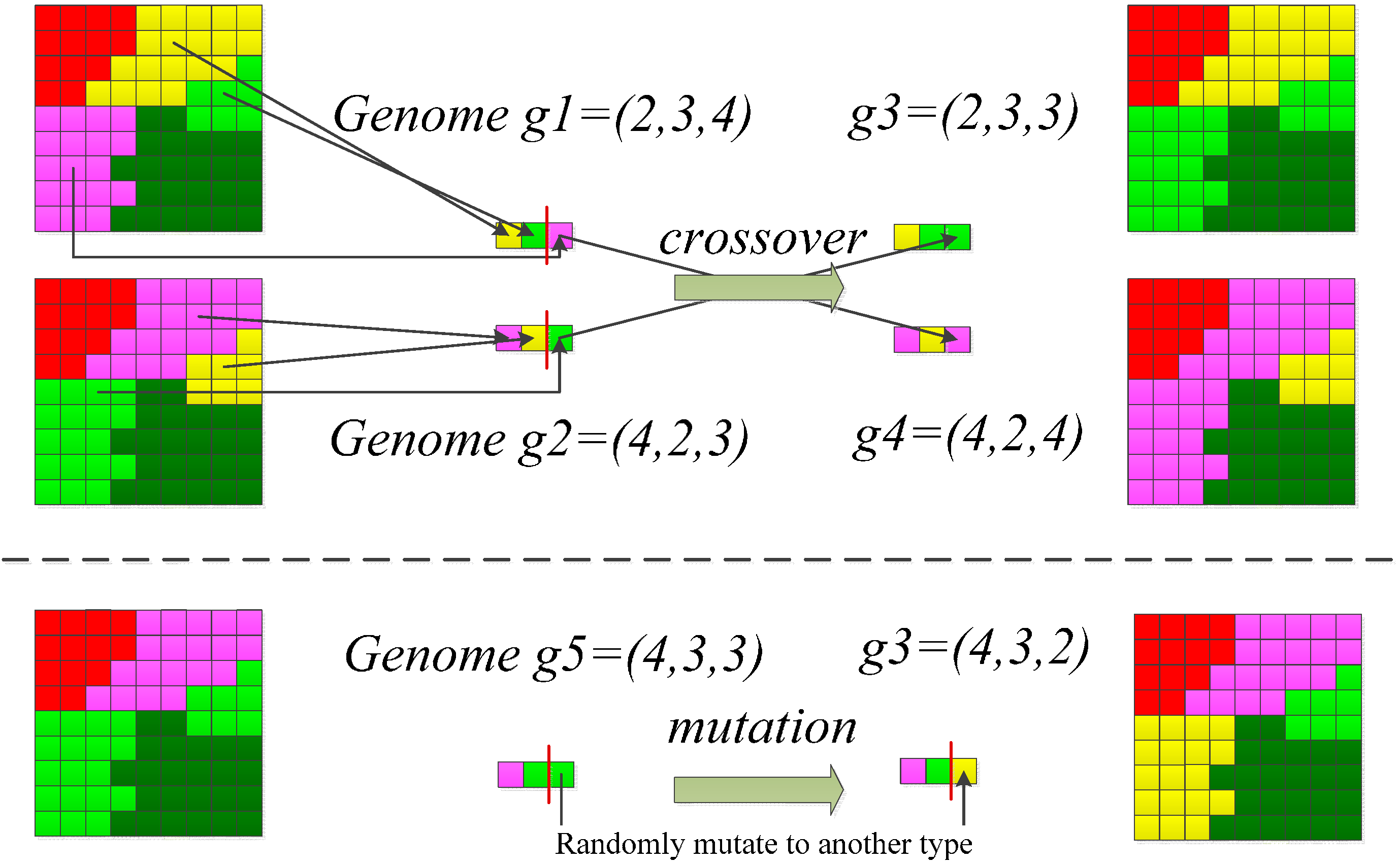
- A population of 100 candidate solutions of the landscape pattern was randomly generated. A candidate solution is represented using a chromosome in the GA. A chromosome indicates a vector of the spatial configuration of a landscape (Figure 2).
- Step 2
- The fitness (objective score) of each candidate landscape pattern was evaluated based on the resultant average habitat suitability index HSImean, which was itself based on a roaming window analysis of landscape metrics.
- Step 3
- Improvement between iterations (i.e., GA-generations) towards an optimal solution was achieved by two genetic operators, the crossover and mutation (Figure 2). The crossover and mutation operator carried on exchanges of patches in the landscape based crossover and mutation rates of 0.5 and 0.01, respectively.
- Step 4
- The iteration stopped when it sought the best solution of 1500 iterations, or while the deviation between the 300 previous generations with the current generation was less than 0.01% (such that the convergence ratio equals 0.9999). Steps 2 and 3 were repeated until the criteria were reached.
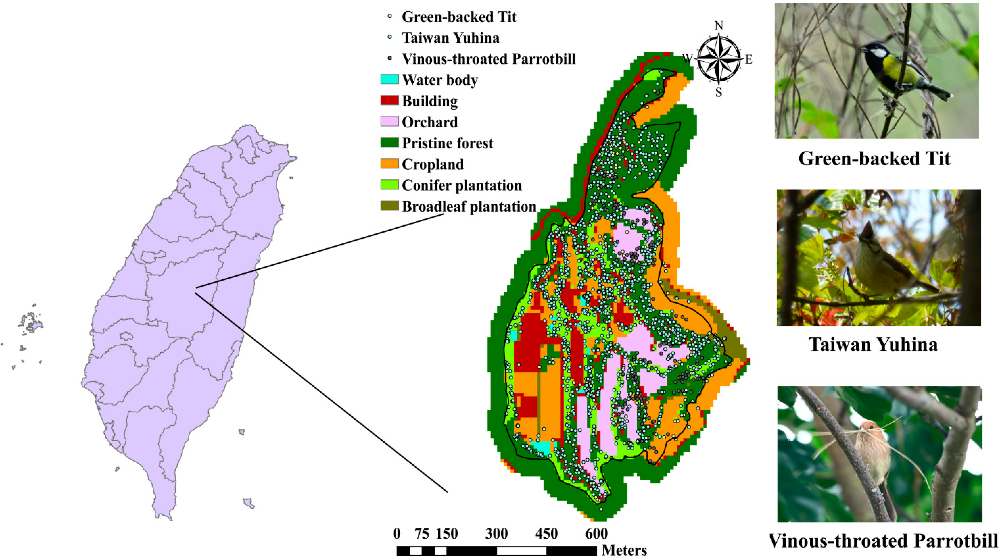
2.3. Study Site and Data Description
3. Results
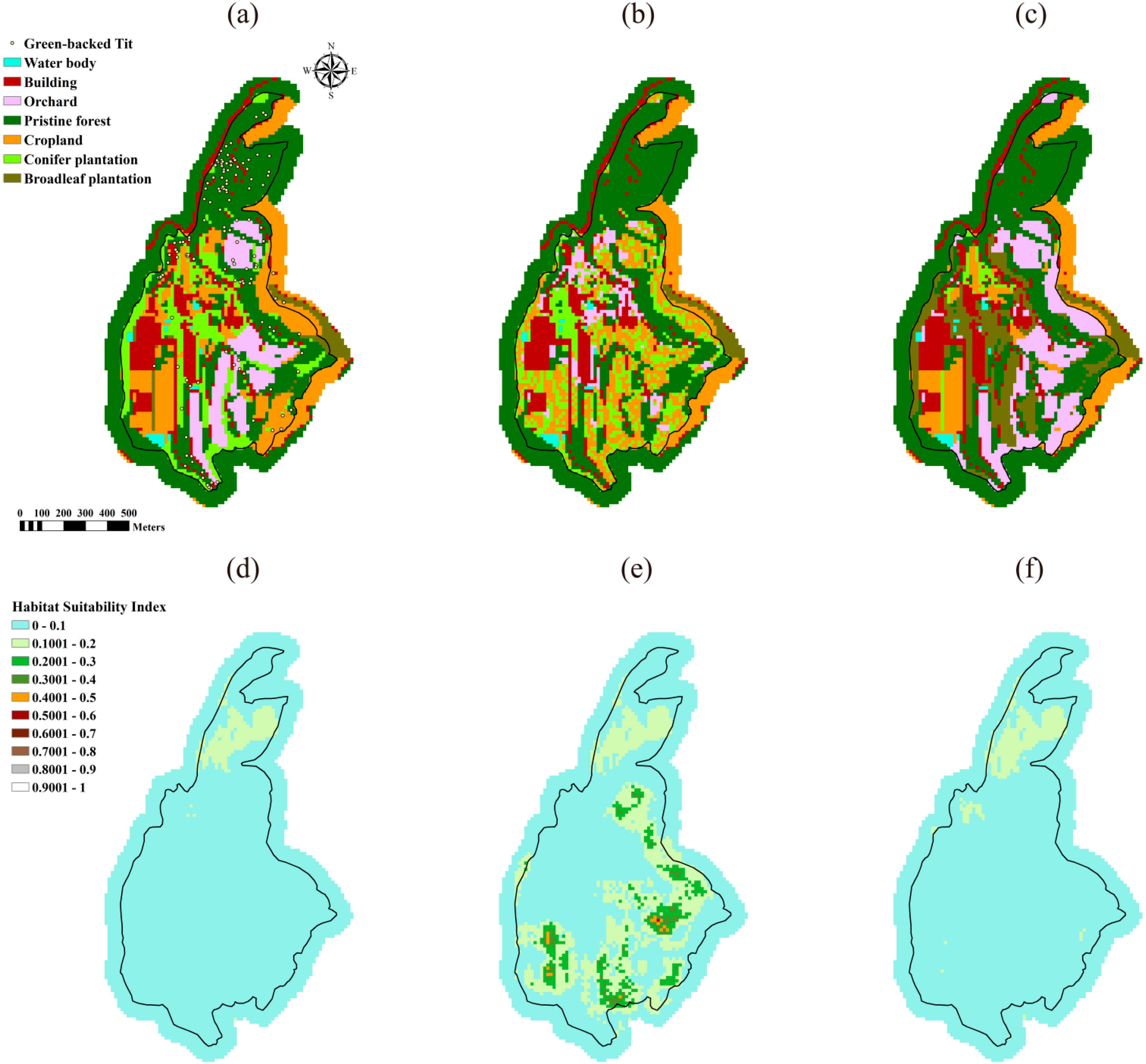
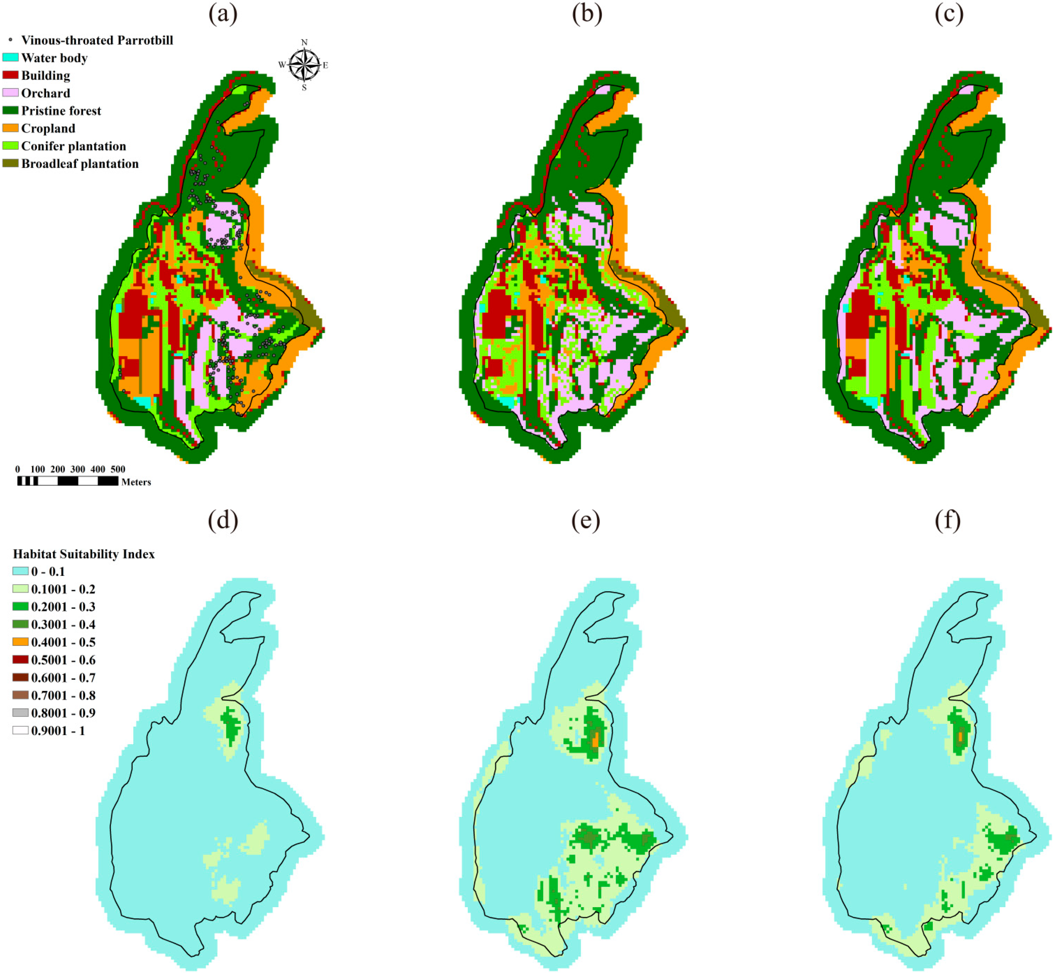
3.1. Optimal Landscapes Resulted from the DDSLOP and LUPOlib Model

| Habitat Suitability | Case 1 the Green-Backed Tit | Case 2 the Taiwan Yuhina | Case 3 the Vinous-Throated Parrotbill | ||||||
|---|---|---|---|---|---|---|---|---|---|
| Current Landscape | DDSLOP | LUPOlib | Current Landscape | DDSLOP | LUPOlib | Current Landscape | DDSLOP | LUPOlib | |
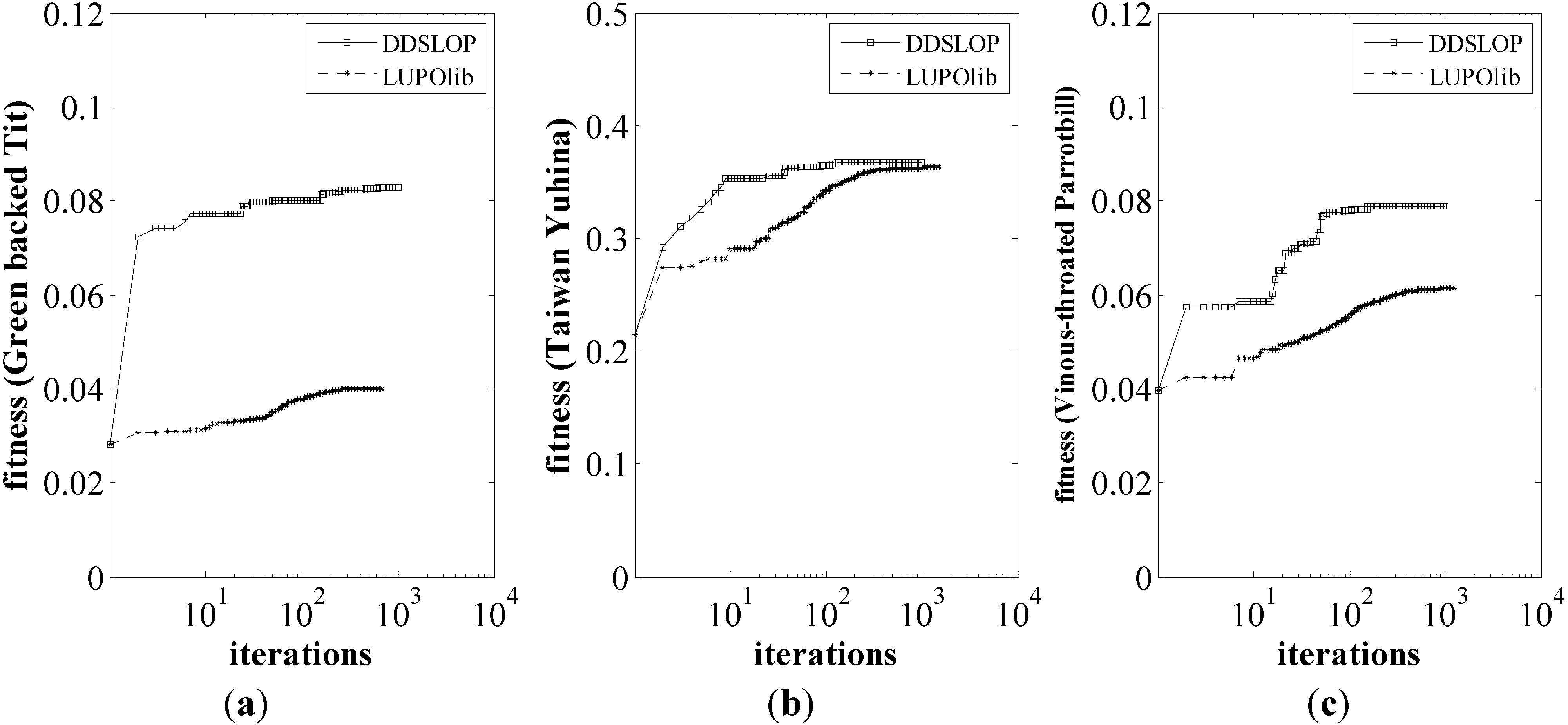
| Average a | 0.0282 | 0.0829 | 0.0432 b | 0.2147 | 0.3668 | 0.3630 | 0.0397 | 0.0789 | 0.0613 |
| Min | 0.0013 | 0.0014 | 0.0026 | 0.0006 | 0.0006 | 0.0006 | 0.0002 | 0.0005 | 0.0005 |
| 25% | 0.0105 | 0.0315 | 0.0190 | 0.1014 | 0.1781 | 0.1652 | 0.0106 | 0.0223 | 0.0190 |
| 50% | 0.0193 | 0.0650 | 0.0312 | 0.2072 | 0.3725 | 0.3532 | 0.0321 | 0.0582 | 0.0445 |
| 75% | 0.0336 | 0.1139 | 0.0521 | 0.3137 | 0.5367 | 0.5527 | 0.0553 | 0.1193 | 0.0825 |
| Max | 0.1601 | 0.5071 | 0.1601 | 0.7389 | 0.8774 | 0.8641 | 0.3392 | 0.4866 | 0.4512 |

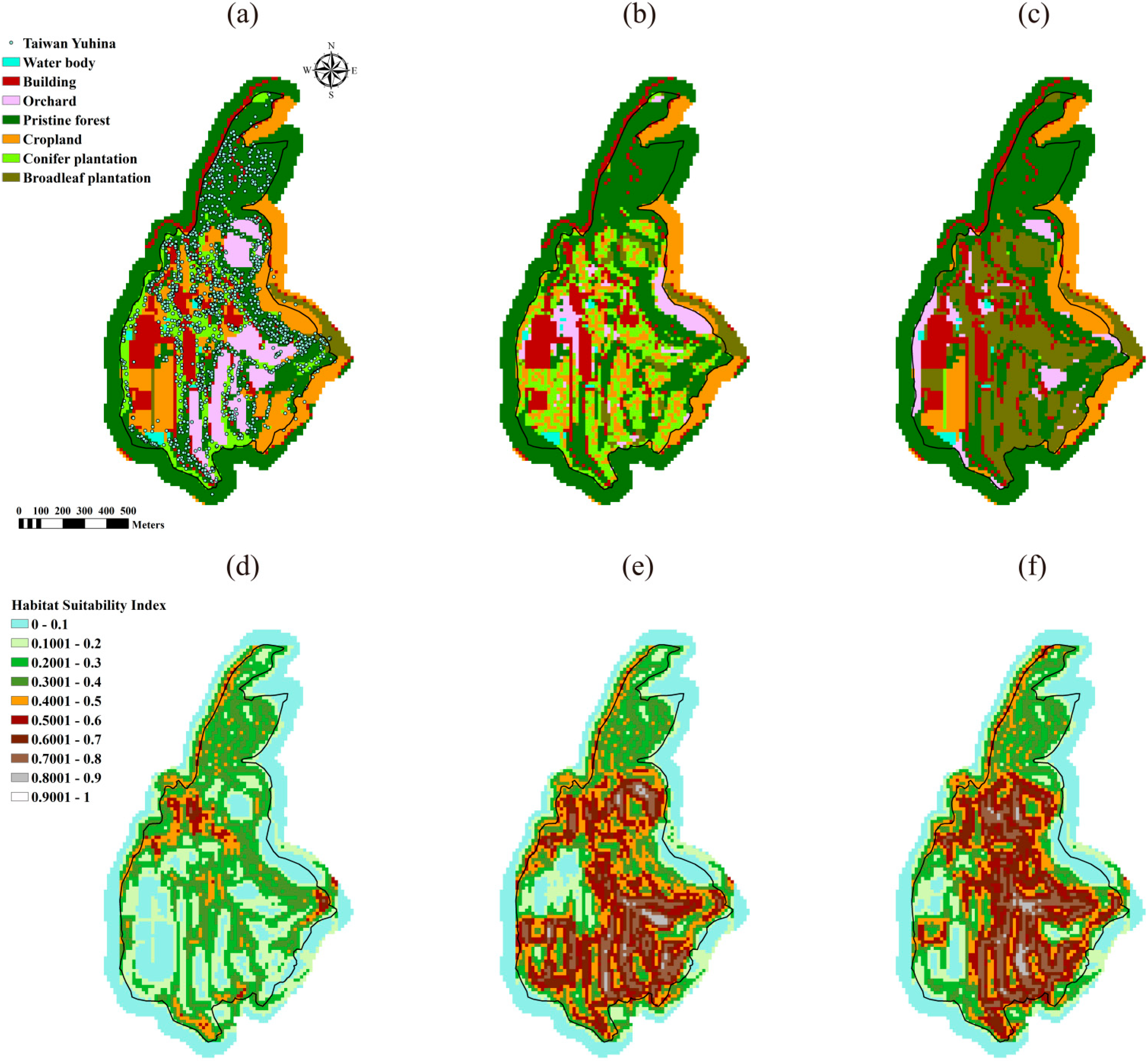

3.2. Preferred Habitat Structures of Target Species
| Drivers | Green-Backed Tit | Taiwan Yuhina | Vinous-Throated Parrotbill | |||
|---|---|---|---|---|---|---|
| Beta | Exp(B) a | Beta | Exp(B) | Beta | Exp(B) | |
| Landscape metrics: | ||||||
| Sum of edge length between building and cropland (esbuildind, cropland) | −0.105 | 0.900 | −0.003 | 0.997 | −0.115 | 0.891 |
| Sum of edge length between building and orchard (esbuildind, orchard) | - | - | - | - | −0.141 | 0.868 |
| Sum of edge length between pristine forest and cropland (esforest, cropland) | −0.089 | 0.915 | - | - | 0.103 | 1.108 |
| Sum of edge length between pristine forest and orchard (esforest, orchard) | - | - | - | - | 0.079 | 1.082 |
| Sum of edge length between cropland and conifer plantation (esorchard, conifer) | 0.14 | 1.150 | 0.062 | 1.064 | - | - |
| Sum of edge length between cropland and broadleaf plantation (escropland, broadleaf) | - | - | −0.066 | 0.936 | - | - |
| Sum of edge length between orchard and conifer plantation (esorchard, conifer) | - | - | - | - | 0.07 | 1.073 |
| Cohesion of conifer plantation (cohconifer) | - | - | −0.006 | 0.994 | - | - |
| Cohesion of broadleaf plantation (cohbroadleaf) | - | - | - | - | −0.03 | 0.970 |
| Large patch index (lpi) | - | - | −0.016 | 0.984 | - | - |
| Class area of pristine forest (caforest) | 2.305 | 10.024 | 2.465 | 11.763 | 2.501 | 12.195 |
| Class area of conifer plantation (caconifer) | −3.575 | 0.028 | 3.719 | 41.223 | - | - |
| Class area of broadleaf plantation (cabroadleaf) | - | - | 4.796 | 121.025 | - | - |
| Distance variables: | ||||||
| Distance to building | - | - | - | - | - | - |
| Distance to road | −0.028 | 0.97 | −0.058 | 0.944 | - | - |
| Constant | −3.521 | −0.783 | −4.542 | |||
| Area Under the Curve of ROC (AUC) | 0.75 | 0.70 | 0.78 | |||
3.3. Performance of the DDSLOP and LUPOlib Model

4. Discussions
4.1. Comparison of Optimal Landscape Planning Using the DDSLOP Model and LUPOlib Model
4.2. Spatial Patterns Resultant from the DDSLOP Model
4.3. Conservation Actions for Landscape Management Using the DDSLOP Model
4.4. Evaluation of the DDSLOP Model
5. Conclusions
Supplementary Materials
Acknowledgments
Author Contributions
Conflicts of Interest
References
- Ligmann-Zielinska, A.; Church, R.L.; Jankowski, P. Spatial optimization as a generative technique for sustainable multiobjective land-use allocation. Int. J. Geogr. Inf. Sci. 2008, 22, 601–622. [Google Scholar] [CrossRef]
- Lin, Y.-P.; Verburg, P.H.; Chang, C.-R.; Chen, H.-Y.; Chen, M.-H. Developing and comparing optimal and empirical land-use models for the development of an urbanized watershed forest in taiwan. Landsc. Urban Plan. 2009, 92, 242–254. [Google Scholar] [CrossRef]
- Holzkämper, A.; Lausch, A.; Seppelt, R. Optimizing landscape configuration to enhance habitat suitability for species with contrasting habitat requirements. Ecol. Model. 2006, 198, 277–292. [Google Scholar] [CrossRef]
- Holzkämper, A.; Seppelt, R. Evaluating cost-effectiveness of conservation management actions in an agricultural landscape on a regional scale. Biol. Conserv. 2007, 136, 117–127. [Google Scholar] [CrossRef]
- Westphal, M.I.; Field, S.A.; Possingham, H.P. Optimizing landscape configuration: A case study of woodland birds in the mount lofty ranges, south australia. Landsc. Urban Plan. 2007, 81, 56–66. [Google Scholar] [CrossRef]
- Lin, Y.-P.; Huang, C.-W.; Ding, T.-S.; Wang, Y.-C.; Hsiao, W.-T.; Crossman, N.D.; Lengyel, S.; Lin, W.-C.; Schmeller, D.S. Conservation planning to zone protected areas under optimal landscape management for bird conservation. Environ. Model. Softw. 2014, 60, 121–133. [Google Scholar] [CrossRef]
- Ball, I.; Possingham, H. Marine Reserve Design Using Spatially Explicit Annealing: A Manual. Available online: http://www.marineplanning.org/pdf/marxan_manual_1_8_2.pdf (accessed on 2 December 2014).
- Moilanen, A. Landscape zonation, benefit functions and target-based planning: Unifying reserve selection strategies. Biol. Conserv. 2007, 134, 571–579. [Google Scholar] [CrossRef]
- Loonen, W.; Heuberger, P.; Kuijpers-Linde, M. Spatial optimisation in land-use allocation problems. In Modelling Land-Use Change; Springer: Berlin, German, 2007; pp. 147–165. [Google Scholar]
- Loman, J.; Schantz, T. Birds in a farmland—More species in small than in large habitat island. Conserv. Biol. 1991, 5, 176–188. [Google Scholar] [CrossRef]
- Loman, J. Small habitat islands are inferior breeding habitats but are used by some great tits—Competition or ignorance? Biodivers. Conserv. 2003, 12, 1467–1479. [Google Scholar] [CrossRef]
- Zakaria, M.; Rajpar, M.N.; Moradi, H.V.; Rosli, Z. Comparison of understorey bird species in relation to edge-interior gradient in an isolated tropical rainforest of malaysia. Environ. Dev. Sustain. 2014, 16, 375–392. [Google Scholar] [CrossRef]
- Tscharntke, T.; Steffan-Dewenter, I.; Kruess, A.; Thies, C. Contribution of small habitat fragments to conservation of insect communities of grassland-cropland landscapes. Ecol. Appl. 2002, 12, 354–363. [Google Scholar]
- Haenke, S.; Kovács-Hostyánszki, A.; Fründ, J.; Batáry, P.; Jauker, B.; Tscharntke, T.; Holzschuh, A. Landscape configuration of crops and hedgerows drives local syrphid fly abundance. J. Appl. Ecol. 2014, 51, 505–513. [Google Scholar] [CrossRef]
- Moilanen, A.; Possingham, H.P.; Polasky, S. A mathematical classification of conservation prioritization problems. In Spatial Conservation Prioritization: Quantitative Methods & Computational Tools; Moilanen, A., Wilson, K.A., Possingham, H.P., Eds.; Oxford University Press: Oxford, UK, 2009; pp. 28–42. [Google Scholar]
- Tolson, B.A.; Shoemaker, C.A. Dynamically dimensioned search algorithm for computationally efficient watershed model calibration. Water Resour. Res. 2007. [Google Scholar] [CrossRef]
- Lozano, M.; García-Martínez, C. Hybrid metaheuristics with evolutionary algorithms specializing in intensification and diversification: Overview and progress report. Comput. Oper. Res. 2010, 37, 481–497. [Google Scholar] [CrossRef]
- McGraigal, K.C.; Samuel, A. The gradient concept of landscape structure. In Issues and Perspectives in Landscape Ecology; Wiens, J.A., Moss, M.R., Eds.; Cambridge University Press: Cambridge, UK, 2005; pp. 112–119. [Google Scholar]
- Tolson, B.A.; Shoemaker, C.A. Efficient prediction uncertainty approximation in the calibration of environmental simulation models. Water Resour. Res. 2008. [Google Scholar] [CrossRef]
- Matott, L.S.; Leung, K.; Sim, J. Application of matlab and python optimizers to two case studies involving groundwater flow and contaminant transport modeling. Comput. Geosci. 2011, 37, 1894–1899. [Google Scholar] [CrossRef]
- Lin, C.-W.; Hsu, F.-H.; Ding, T.-S. Applying a territory mapping method to census the breeding bird community composition in a montane forest of taiwan. Taiwan J. For. Sci. 2011, 26, 267–285. [Google Scholar]
- Westphal, M.I.; Pickett, M.; Getz, W.M.; Possingham, H.P. The use of stochastic dynamic programming in optimal landscape reconstruction for metapopulations. Ecol. Appl. 2003, 13, 543–555. [Google Scholar] [CrossRef]
- Villard, M.A.; Metzger, J.P. Review: Beyond the fragmentation debate: A conceptual model to predict when habitat configuration really matters. J. Appl. Ecol. 2014, 51, 309–318. [Google Scholar] [CrossRef]
- Reid, J.L.; Mendenhall, C.D.; Rosales, J.A.; Zahawi, R.A.; Holl, K.D. Landscape context mediates avian habitat choice in tropical forest restoration. PLoS One 2014, 9, e90573. [Google Scholar] [CrossRef] [PubMed]
- Graham, L.L.; Page, S.E. Artificial bird perches for the regeneration of degraded tropical peat swamp forest: A restoration tool with limited potential. Restor. Ecol. 2012, 20, 631–637. [Google Scholar] [CrossRef]
- Pouzols, F.M.; Burgman, M.A.; Moilanen, A. Methods for allocation of habitat management, maintenance, restoration and offsetting, when conservation actions have uncertain consequences. Biol. Conserv. 2012, 153, 41–50. [Google Scholar] [CrossRef]
- Lindenmayer, D.; Knight, E.; Crane, M.; Montague-Drake, R.; Michael, D.; MacGregor, C. What makes an effective restoration planting for woodland birds? Biol. Conserv. 2010, 143, 289–301. [Google Scholar] [CrossRef]
- Grainger, M.J.; van Aarde, R.J.; Wassenaar, T.D. Landscape composition influences the restoration of subtropical coastal dune forest. Restor. Ecol. 2011, 19, 111–120. [Google Scholar] [CrossRef]
- Cole, R.J.; Holl, K.D.; Zahawi, R.A. Seed rain under tree islands planted to restore degraded lands in a tropical agricultural landscape. Ecol. Appl. 2010, 20, 1255–1269. [Google Scholar] [CrossRef] [PubMed]
- Wagner, H.H.; Fortin, M.-J. Spatial analysis of landscapes: Concepts and statistics. Ecology 2005, 86, 1975–1987. [Google Scholar] [CrossRef]
- Buckland, S.; Cole, N.C.; Aguirre-Gutiérrez, J.; Gallagher, L.E.; Henshaw, S.M.; Besnard, A.; Tucker, R.M.; Bachraz, V.; Ruhomaun, K.; Harris, S.; et al. Ecological effects of the invasive giant madagascar day gecko on endemic mauritian geckos: Applications of binomial-mixture and species distribution models. PLoS One 2014, 9, e88798. [Google Scholar] [CrossRef] [PubMed]
- Pedrana, J.; Bernad, L.; Maceira, N.O.; Isacch, J. Human-sheldgeese conflict in agricultural landscapes: Effects of environmental and anthropogenic predictors on sheldgeese distribution in the southern pampa, argentina. Agric. Ecosyst. Environ. 2014, 183, 31–39. [Google Scholar] [CrossRef]
© 2014 by the authors; licensee MDPI, Basel, Switzerland. This article is an open access article distributed under the terms and conditions of the Creative Commons Attribution license (http://creativecommons.org/licenses/by/4.0/).
Share and Cite
Huang, C.-W.; Lin, Y.-P.; Ding, T.-S.; Anthony, J. Developing a Cell-Based Spatial Optimization Model for Land-Use Patterns Planning. Sustainability 2014, 6, 9139-9158. https://doi.org/10.3390/su6129139
Huang C-W, Lin Y-P, Ding T-S, Anthony J. Developing a Cell-Based Spatial Optimization Model for Land-Use Patterns Planning. Sustainability. 2014; 6(12):9139-9158. https://doi.org/10.3390/su6129139
Chicago/Turabian StyleHuang, Chun-Wei, Yu-Pin Lin, Tzung-Su Ding, and Johnathen Anthony. 2014. "Developing a Cell-Based Spatial Optimization Model for Land-Use Patterns Planning" Sustainability 6, no. 12: 9139-9158. https://doi.org/10.3390/su6129139
APA StyleHuang, C.-W., Lin, Y.-P., Ding, T.-S., & Anthony, J. (2014). Developing a Cell-Based Spatial Optimization Model for Land-Use Patterns Planning. Sustainability, 6(12), 9139-9158. https://doi.org/10.3390/su6129139