The Impact of Green Space Changes on Air Pollution and Microclimates: A Case Study of the Taipei Metropolitan Area

Abstract
:1. Introduction
2. Research Design
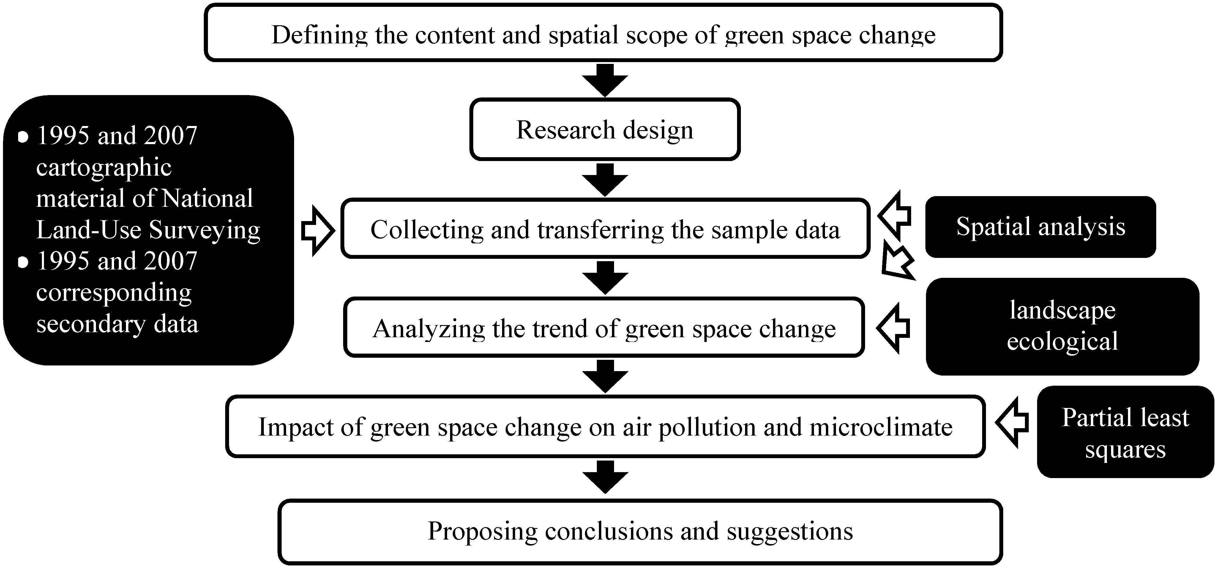
2.1. Analytical Framework
- (1)
- Defining the content and the spatial scope of green space changes: Confirm the research category and scope of green space change.
- (2)
- Developing the research design: Determine the method, variables and hypotheses based on the theme and purposes of this study.
- (3)
- Collecting and transferring the sample data: Collect and convert corresponding secondary data and cartographic material of the National Land-Use Survey from 1995 and 2007 through spatial analysis.
- (4)
- Analyze the trend of green space change: Identify the state of green space change and migration between different land uses through land transfer matrix and spatial analysis. Additionally, analyze the spatial structure/composition change of green space through landscape ecology metrics.
- (5)
- Discovering the impact of green space change on air pollution and the microclimate: Analyze the effect of green space change on air pollution and the microclimate, and identify the critical effect through partial least squares (PLS).
- (6)
- Proposing conclusions and corresponding suggestions.
2.2. Method
2.2.1. Spatial Analysis
2.2.2. Landscape Ecological Metrics
2.2.3. Partial Least Squares
2.3. Definition of Variables and Hypotheses
2.3.1. Green Space Change Analysis
2.3.2. Impact of Green Space Change

| Perspective | Latent Variables | Latent Variables Code | Observed Variables | Observed Variables Code |
|---|---|---|---|---|
| change of green space | change of Landscape | CL |
| cPLAND cWAERA |
| change of fragmentation | CF |
| cNP cPD cSPLIT | |
| change of aggregation | CA |
| cPLADJ cCLUMPY cAI | |
| change of area | CR |
| cAREA-MN cAREA-AM | |
| change of proximity | CN |
| cENN-MN cENN-AM | |
| change of largest patch percentage | CP |
| cLPI | |
| change of air pollution | change of air pollution emission | CAP |
| SO2 NOx PM CO2 NO NO2 |
| change of microclimate | change of rainfall type | CRT |
| Rain lrd brd nrd |
| change of temperature | CST |
| Temp |
| Endogenous latent variables/exogenous latent variables | Change of Landscape | Change of fragmentation | Change of aggregation | Change of area | Change of proximity | Change of largest patch percentage | Change of air pollution emission |
|---|---|---|---|---|---|---|---|
| change of air pollution emission | − | + | − | − | + | − | none |
| change of rainfall type | − | + | − | − | + | − | +/− |
| change of temperature | − | + | − | − | + | − | +/− |
3. Data
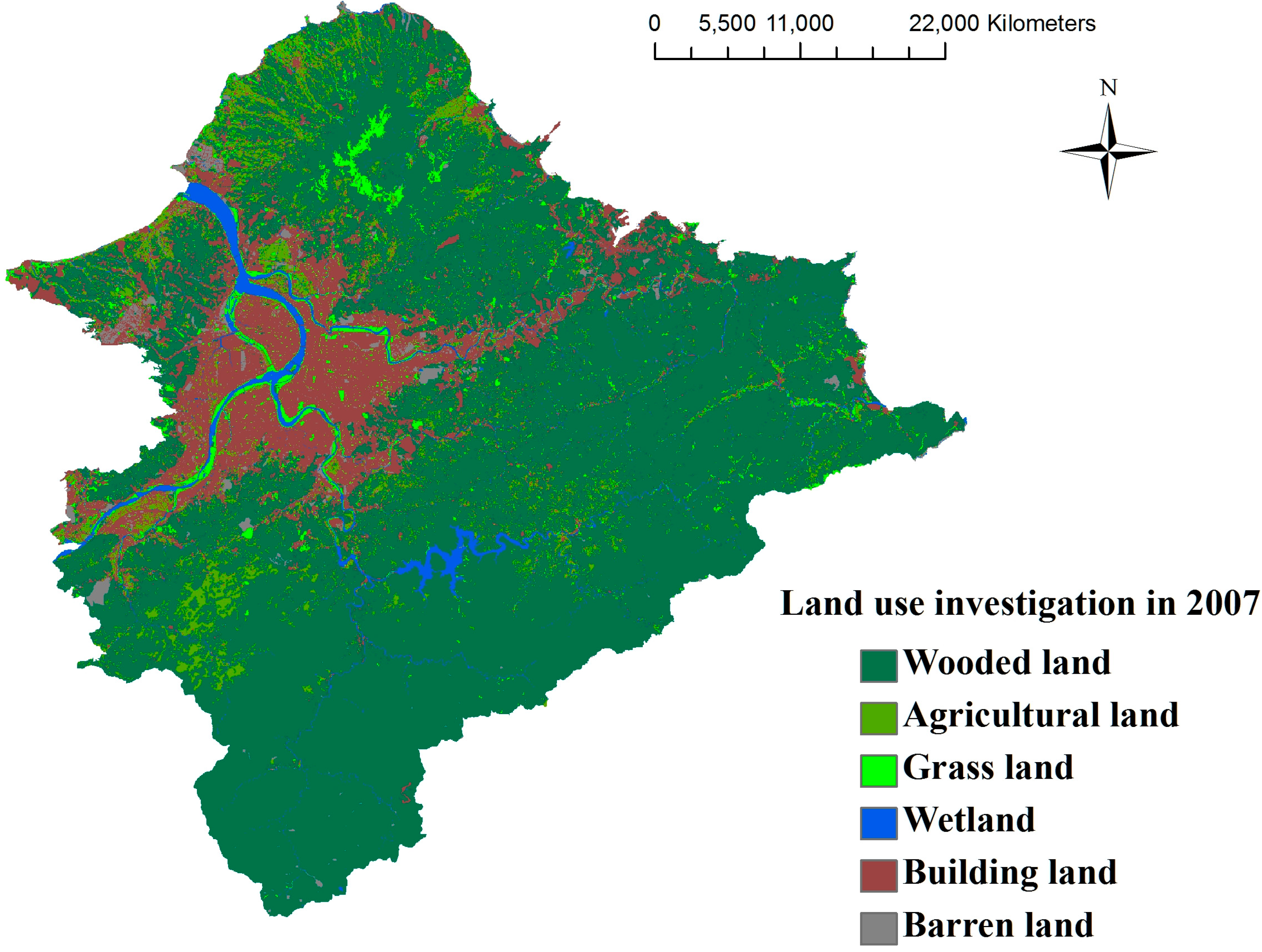
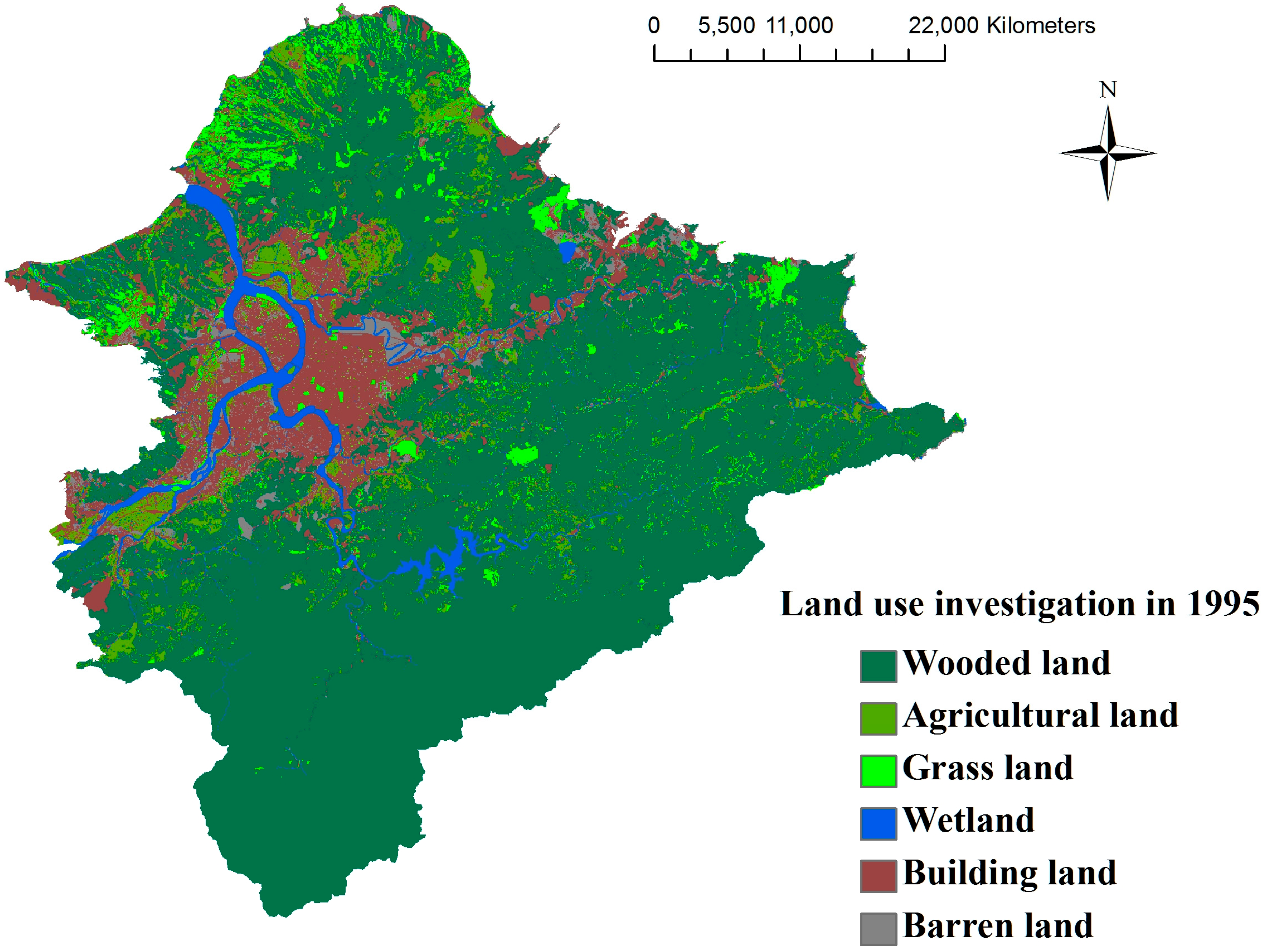
3.1. Empirical Area
3.2. Description of the Empirical Sample

4. Trend of Green Space Change
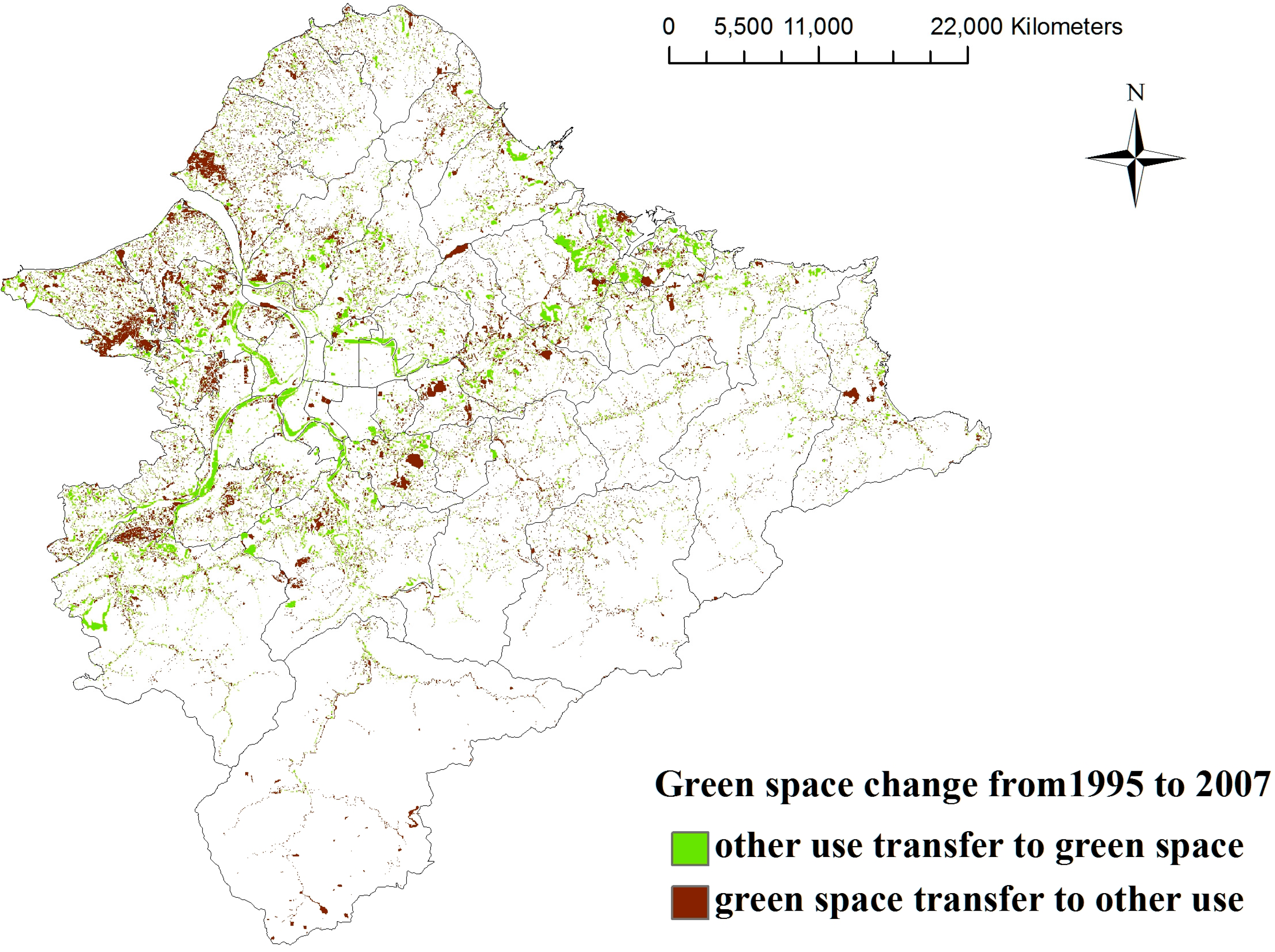
4.1. States of Green Space Changes
| Land use area in 1995 | Land use area in 2007 | ||||||||
|---|---|---|---|---|---|---|---|---|---|
| Green space | Wetland | Building land | Barren land | Total | |||||
| Wooded land | Agricultural land | Grass land | Total | ||||||
| Green space | Wooded land | 150,204.5 | 6524.5 | 2333.5 | 159,062.5 | 953.75 | 4989.25 | 1198 | 166,203.5 |
| Agricultural land | 7917 | 6591.25 | 874 | 15,382.25 | 279 | 2975.25 | 648.5 | 19,285 | |
| Grass land | 5056.5 | 2036.25 | 1224 | 8316.75 | 186.5 | 1592.25 | 537 | 10,632.5 | |
| Total | 163178 | 15152 | 4431.5 | 182,761.5 | 1419.25 | 9556.75 | 2383.5 | 196,121 | |
| Wetland | 1735.75 | 532.75 | 1326.5 | 3595 | 4877.5 | 1297.5 | 287.25 | 10,057.25 | |
| Building land | 384.25 | 491.5 | 503.25 | 1379 | 283.75 | 25,376 | 1201.75 | 28,240.5 | |
| Barren land | 1995.5 | 360.25 | 702.75 | 3058.5 | 188 | 2953.5 | 721.5 | 6921.5 | |
| Total | 167,293.5 | 16,536.5 | 6964 | 190,794 | 6768.5 | 39,183.75 | 4594 | 241340.3 | |
| Area change | 1090 | −2748.5 | −3668.5 | −5327 | −3288.75 | 10,943.25 | −2327.5 | - | |

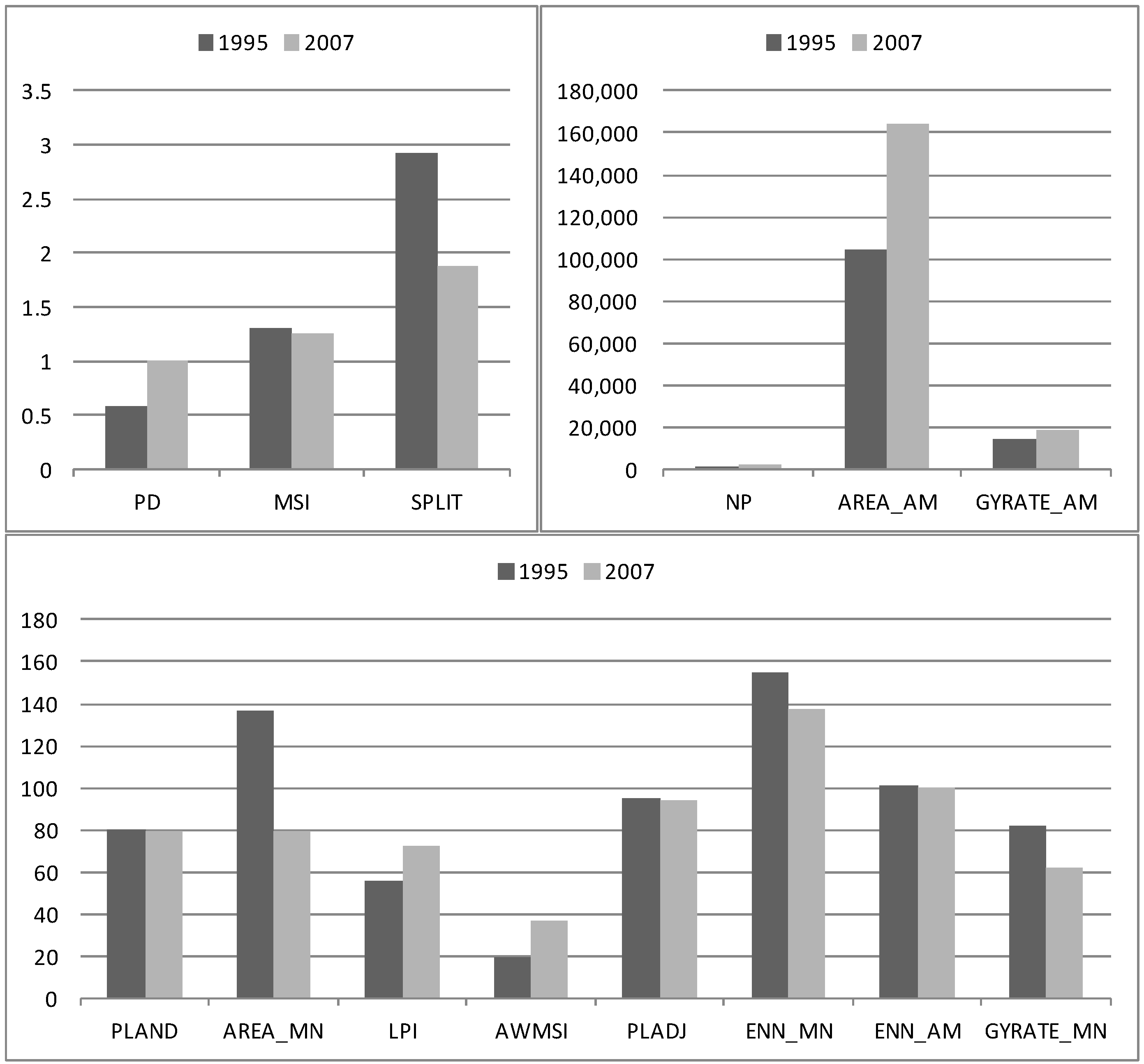
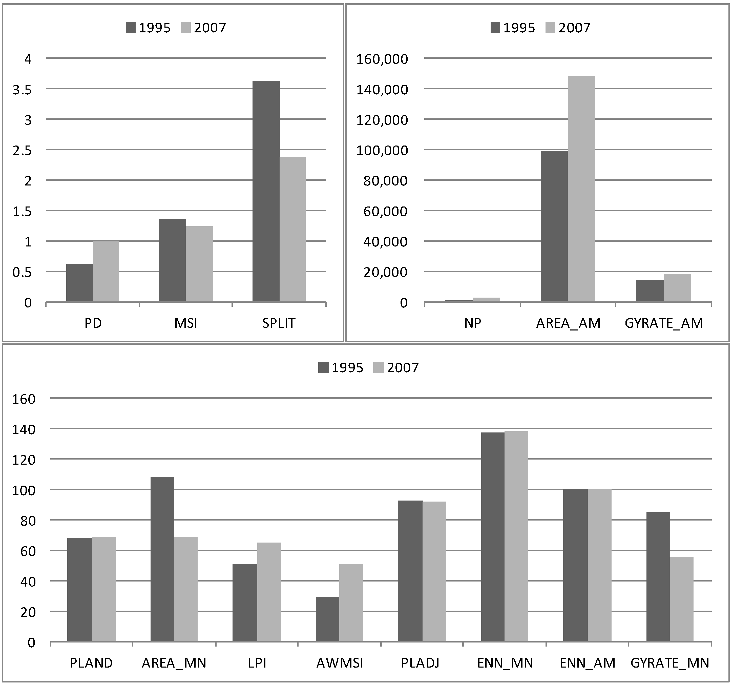
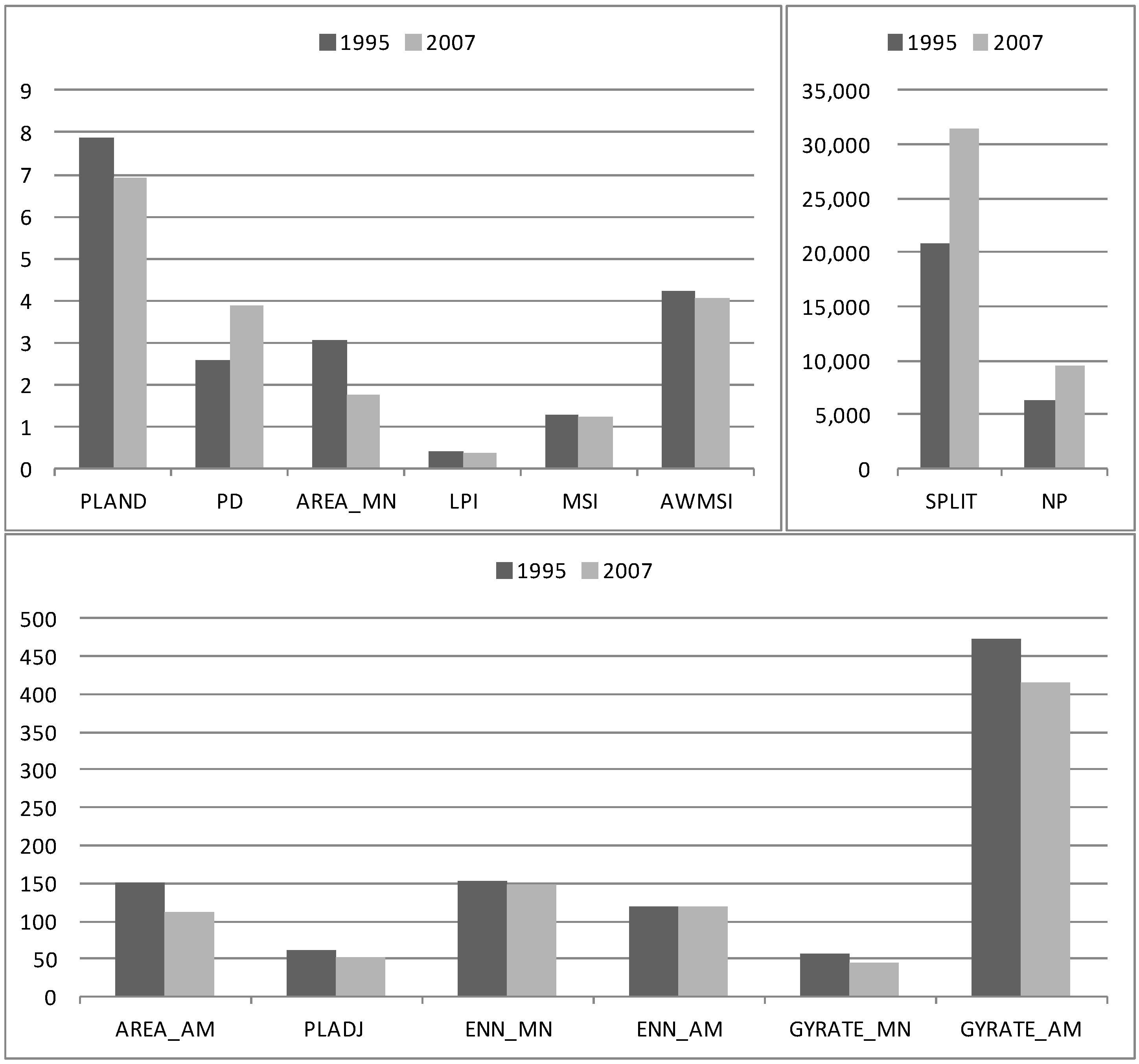
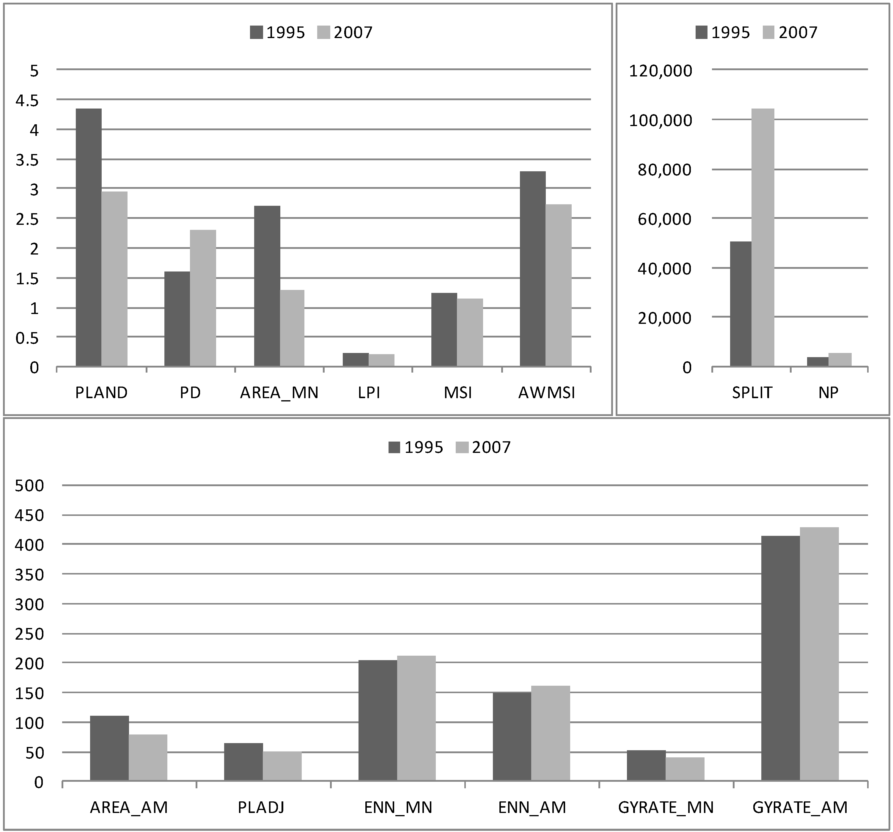
4.2. Results of Landscape Ecological Metrics
| landscape ecological metrics | Green space | Wooded land | Agricultural land | Grass land | ||||
|---|---|---|---|---|---|---|---|---|
| 1995 | 2007 | 1995 | 2007 | 1995 | 2007 | 1995 | 2007 | |
| PLAND | 80.11 | 79.15 | 67.89 | 69.27 | 7.88 | 6.93 | 4.34 | 2.96 |
| NP | 1433 | 2450 | 1531 | 2456 | 6313 | 9524 | 3918 | 5637 |
| PD | 0.59 | 1.00 | 0.63 | 1.00 | 2.58 | 3.89 | 1.60 | 2.30 |
| AREA_MN | 136.86 | 79.10 | 108.56 | 69.045 | 3.05 | 1.78 | 2.71 | 1.28 |
| AREA_AM | 104,529.1 | 164,396.1 | 99,271.33 | 148,504.8 | 149.67 | 112.62 | 111.06 | 79.44 |
| LPI | 55.81 | 72.85 | 51.28 | 64.8 | 0.4 | 0.38 | 0.22 | 0.21 |
| MSI | 1.31 | 1.26 | 1.36 | 1.25 | 1.30 | 1.23 | 1.24 | 1.15 |
| AWMSI | 19.59 | 36.59 | 30.11 | 51.33 | 4.24 | 4.06 | 3.30 | 2.73 |
| PLADJ | 95.41 | 93.90 | 93.25 | 91.80 | 62.26 | 52.52 | 64.31 | 51.58 |
| ENN_MN | 154.95 | 137.05 | 137.52 | 138.41 | 152.8 | 148.06 | 203.76 | 210.74 |
| ENN_AM | 100.65 | 100.35 | 100.63 | 100.41 | 119.2 | 120.48 | 148.80 | 162.10 |
| SPLIT | 2.92 | 1.88 | 3.63 | 2.38 | 20,767.1 | 31,379.9 | 50,762 | 104,239 |
| GYRATE_MN | 81.61 | 62.37 | 85.15 | 55.8 | 56.08 | 45.68 | 52.7 | 41 |
| GYRATE_AM | 14,120.05 | 18,448.3 | 14,408.84 | 18,302.39 | 472.2 | 414.56 | 413.53 | 429.23 |
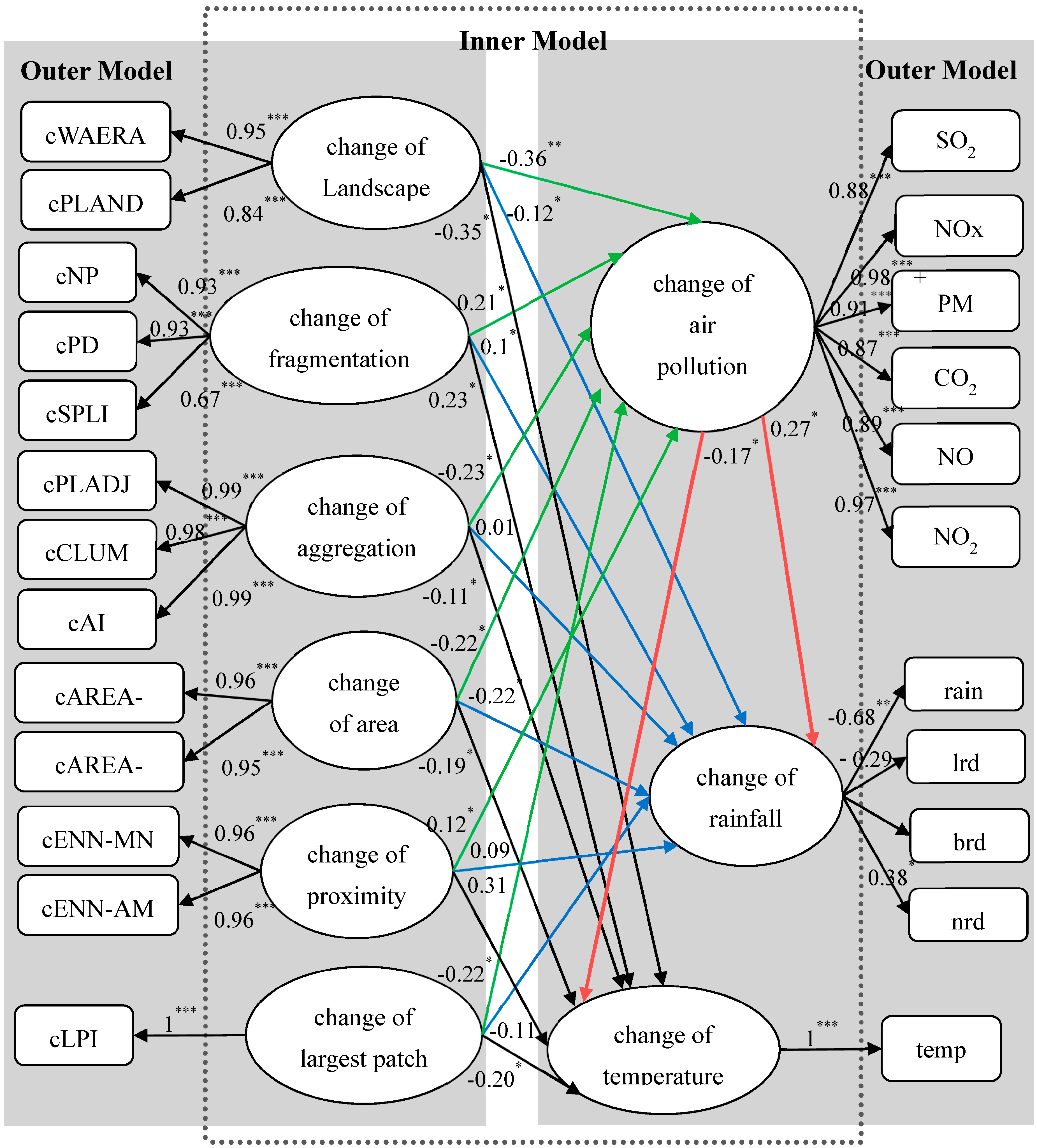
5. Impact of Green Space Change
5.1. Model Calibrations and Verifications
| Perspective | Latent Variables | Observed Variables | Loadings | Z-value | Significance |
|---|---|---|---|---|---|
| change of green space | change of Landscape | ● change of PLAND | 0.849 | 4.186 | *** |
| change of fragmentation | ● change of NP | 0.933 | 9.461 | *** | |
| change of aggregation | ● change of PLADJ | 0.996 | 11.101 | *** | |
| change of area | ● change of AREA-MN | 0.966 | 14.067 | *** | |
| change of proximity | ● change of ENN-MN | 0.967 | 5.544 | *** | |
| change of largest patch percentage | ● change of LPI | 1.000 | - | ||
| change of air pollution | change of air pollution emission | ● change of SO2 emission | 0.888 | 30.560 | *** |
| change of microclimate | change of rainfall type | ● change of mean annual rainfall | -0.686 | 2.909 | ** |
| change of temperature | ● change of mean annual temperature | 1.000 | - |
| Perspective | Latent Variables | Cronbach’s α | CR a | Average | R Square |
|---|---|---|---|---|---|
| change of green space | change of Landscape | 0.892 | 0.907 | 0.895 | |
| change of fragmentation | 0.818 | 0.854 | 0.841 | ||
| change of aggregation | 0.991 | 0.994 | 0.982 | ||
| change of area | 0.913 | 0.958 | 0.919 | ||
| change of proximity | 0.927 | 0.965 | 0.932 | ||
| change of largest patch percentage | 1.000 | 1.000 | 1.000 | ||
| change of air pollution | change of air pollution emission | 0.965 | 0.972 | 0.883 | 0.479 |
| change of microclimate | change of rainfall type | 0.701 | 0.718 | 0.699 | 0.328 |
| Endogenous latent variables/exogenous latent variables | Change of Landscape | Change of fragmentation | Change of aggregation | Change of area | Change of proximity | Change of largest patch percentage | Change of air pollution emission |
|---|---|---|---|---|---|---|---|
| change of air pollution emission | −0.3619 ** | 0.2067 * | −0.2268 * | −0.2158 * | 0.1161 * | −0.2211 * | - |
| change of rainfall type | −0.1162 * | 0.1028 * | 0.0088 | −0.1042 * | 0.0949 | −0.1076 | 0.2726 * |
| change of temperature | −0.3523 * | 0.2328 * | −0.1108 * | −0.1912 * | 0.3148 | −0.2022 * | −0.1707 * |
5.2. Results Analysis
6. Conclusions and Suggestions
- (1)
- According to the analytical results, the green space area within the Taipei Metropolitan Areas has decreased 1.19% from 1995 to 2007, but 93.19% of the green space area have kept their original purposes.
- (2)
- The results of landscape ecological metrics show the more fragmented trend of the green space. Regarding the change of the green space area, the large patch area is shown as increasing and the small patch area as decreasing. Regarding the change of the green space shape, the shape of the entire green space is shown as tending toward being simple, while the shape of the large patch tends toward being complex. The changes in green space aggregation mean that green space is still highly centralized. The changes in green space proximity represent the distribution of the entire green space tending toward aggregation, and the distribution of the large patch shows no change. The changes in green space extendibility demonstrate the connection between the large patch increase and the small patch reduction, as it closely relates to the area changes of the large and small patches.
- (3)
- The results from the PLS model indicate that the changing pattern of green space area has a great influence on air pollution and microclimate patterns. For instance, less air pollution, smaller rainfall patterns, and cooler temperatures are associated with improvements in space aggregation, increasing the large sized green space patch. These results are similar to the research findings by Beatley [9], Jo [10], Yang et al. [11], Shin and Le [15], Herb et al. [16], and Leuzinger et al. [17]. However, they didn’t discuss the patterns of green space, they only emphasized the total areas of green space. Although anthropogenic heat release is one of the important factors affecting air pollution and microclimates [32,36] in urban areas, we would assume that green space changes and anthropogenic heat release increase are major factors affecting the air pollution and microclimate pattern in cities.
- (4)
- According to the results of the PLS model, the air pollution emissions change negatively affects the temperature change because of the cooling effect being higher than the warming effect. These results are similar to the findings by De Oliveira et al. [49], Koronakis et al. [50], and Wei and Hsu [52]. Moreover, the air pollution emission change positively affects the rainfall type change, which means the higher emission of air pollution reduces the occurrence of light rainy days and the mean annual rainfall and increases the number of non-rainy days. These results are consistent with Allen and Ingram [54].
- (1)
- The transfer of green space always occurs in the core area, in the sub-core area, and in the surrounding area. Thus, an urban growth boundary should be designated to avoid urban sprawl and the loss of green space.
- (2)
- The trends and locations of wooded lands , agricultural lands and grass lands are different, and the conservation policies for green space should be adjusted for these different forms. The wooded land in suburbs should be effectively conserved to avoid decreases in the core areas and sub-core areas. Agricultural land should avoid arbitrary releases and transfers to land for development and construction while maintaining the integrity of the land. The grass land should be the focus of concern with regard to its change in the suburbs and sub-central area, and enhanced with conservation to avoid its loss.
- (3)
- Green space has the function of reducing air pollutants, cooling temperatures and improving rainfall types. In addition, green space has the effect of scale and aggregation with regard to these functions. Thus, the development of the green space concept (such as a green city, garden city, green infrastructure) and policy (green space conservation) can be one of the solutions to climate change. Moreover, laws and governmental mechanisms relating to green space should be drafted immediately to help implement green policies.
- (4)
- In this paper, we have only analyzed the changes from 1995 to 2007 due to limitations in data. If sufficient data can be provided in the future, these changes can be analyzed over a longer term.
Acknowledgments
Author Contributions
Appendix
| Indicator | Formula | Units | indicator content and measuring purpose |
|---|---|---|---|
| Percentage of Landscape (PLAND) | aij: area of patch j (class i). A: total landscape area. | % | PLAND equals the percentage the landscape comprised of the corresponding patch type. The higher PLAND is, the more important the patch of corresponding class is. This paper use PLAND to analyze the importance of green space in landscape. |
| Number of Patches (NP) | ni ni: number of patches in the landscape of patch type (class) i. | None | NP equals the number of patches of the corresponding patch type. The higher NP is, the more fragmented the patch of corresponding class is. This paper use NP to analyze the fragmentation of green space in landscape. |
| Patch Density (PD) | (ni/A)(10,000)(100) ni, A: definition as before. | Number per 100 hectares | PD equals the percentage the landscape comprised of the patches of the corresponding class. The higher PD is, the more fragmented the patch of corresponding class is. This paper use PD to analyze the fragmentation of green space in landscape. |
| Mean Patch Area (AREA_MN) | aij, ni:definition as above. | Hectares | AREA_MN provides the measure of patch area in corresponding class. The higher AREA_MN is, the larger the patch of corresponding class is. This paper use AREA_MN to analyze the size of green space patch in landscape. |
| Area-Weighted Mean Patch Area (AREA_AM) | aij: definition as before. | Hectares | AREA_AM provides the measure of area-weighted patch area in corresponding class. The higher AREA_ AM is, the larger the patch of corresponding class is. This paper use AREA_MN to analyze the size of green space patch in landscape based on reducing the impact of small patches changes, and to compare with AREA_MN. |
| Largest Patch Index (LPI) | aij, A: definition as before. | % | LPI equals the percentage of the landscape comprised by the largest patch. The higher LPI is, the more important the patch of corresponding class is. This paper use LPI to analyze the contribution of largest patch, and to identify the advantage category in landscape. |
| Mean shape index (MSI) | pij: perimeter of patch j (class i). aij, ni: definition as above. | None | MSI provides the measure of patch shape in corresponding class. The higher MSI is, the more complex the patch shape in corresponding class is. This paper use MSI to analyze the complexity of the green space patch shape in corresponding class. |
| Area-Weighted Mean Shape Index (AWMSI) | pij, aij: definition as above. | None | AWMSI provides the measure of area-weighted patch shape in corresponding class. The higher AWMSI is, the more complex the patch shape in corresponding class is. This paper use AWMSI to analyze the complexity of green space patch in corresponding class based on reducing the impact of small patches changes, and to compare with MSI. |
| Mean Nearest Neighbor Distance (ENN_MN) | hij:distance between patch j (class i) to patch of the corresponding type; n'i:number of patches in the landscape of patch type (class) i which having nearest neighbor distance. | Meter | ENN_MN provides the measure of patch distance in corresponding class. The higher ENN_MN is, the more dissipative the patch in corresponding class is. This paper use ENN_MN to analyze the proximity of each green space patches in corresponding class. |
| Area-Weighted Mean Nearest Neighbor Distance (ENN_AM) | hij, aij:definition as above. | Meter | ENN_AM provides the measure of area-weighted patch distance in corresponding class. The higher ENN_AM is, the more dissipative the patch in corresponding class is. This paper use ENN_AM to analyze the proximity of each green space patches in corresponding class based on reducing the impact of small patches changes, and to compare with ENN_MN. |
| Percentage of Like Adjacencies (PLADJ) | gii: number of like adjacencies between pixels of patch type (class) i based on the double-count method. gik: number of adjacencies between pixels of patch types (classes) i and k based on the double-count method. | % | PLADJ equals the percentage of cell adjacencies involving the corresponding patch type that are like adjacencies. PLADJ equals 0 when the corresponding patch type is maximally disaggregated and there are no like adjacencies. In contrast, The higher of PLADJ means high aggregation of the same type patch. This paper use PLADJ to analyze the aggregation of green space patches in corresponding class. |
| Splitting Index (SPLIT) | aij, A: definition as above. | None | SPLIT provides the measure separation of patch in corresponding class. SPLIT equals 1 when the landscape consists of single patch. SPLIT increases as the focal patch type is increasingly reduced in area and subdivided into smaller patches. This paper use PLADJ to analyze the separation of green space patches in corresponding class. |
| Radius of Gyration (GYRATE_MN) | hijr: distance between cell ijr (located within patch ij) and the centroid of patch ij (the average location), based on cell center to cell center distance. z: number of cells in patch ij. | Meter | GYRATE_MN provides the measure of patch connection and extendibility in corresponding class. The higher GYRATE_MN is, the more connected the patch in corresponding class is. This paper use GYRATE_MN to analyze the connection of green space patch in corresponding class. |
| Area-Weighted Radius of Gyration (GYRATE_AM) | hijr, aij, z: definition as above. | Meter | GYRATE_AM provides the measure of area-weighted patch connection in corresponding class. The higher GYRATE_AM is, the more connected the patch in corresponding class is. This paper use GYRATE_AM to analyze the connection of green space patch in corresponding class based on reducing the impact of small patches changes, and to compare with GYRATE_MN. |
| Clumpiness Index (CLUMPY) | Pi: proportion of the landscape occupied by patch type (class) i. min ei: minimize the perimeter under the compact patch type (class) i of fixed grid number. gii, gik: definition as above. | None | CLUMPY provides the measure of patch aggregation in corresponding class. CLUMPY equals -1 when the focal patch type is maximally disaggregated. CLUMPY equals 0 when the focal patch type is distributed randomly, and approaches 1 when the patch type is maximally aggregated. This paper use CLUMPY to analyze the aggregation of green space patch in corresponding class. |
| Aggregation Index (AI) | gss: number of like adjacencies between pixels of patch type (class) s based on the single-count method. max→gss: maximum number of like adjacencies between pixels of patch type (class) s based on the single-count method. | % | AI provides the measure of patch aggregation in corresponding class. AI equals 0 when the focal patch type is maximally disaggregated. AI increases as the focal patch type is increasingly aggregated and equals 100 when the patch type is maximally aggregated into a single, compact patch. This paper use AI to analyze the aggregation of green space patch in corresponding class. |


Conflicts of Interest
References
- Parry, M.L.; Canziani, O.F.; Palutikof, J.P.; van der Linden, P.J.; Hanson, C.E. Climate Change 2007: Impacts, Adaptation and Vulnerability—Working Group II Contribution to IPCC Fourth Assessment Report; Cambridge University Press: Cambridge, UK, 2007. [Google Scholar]
- Metz, B.; Davidson, O.R.; Bosch, P.R.; Dave, R. Climate Change 2007: Mitigation of Climate Change—Working Group III Contribution to IPCC Fourth Assessment Report; Cambridge University Press: Cambridge, UK, 2007. [Google Scholar]
- Tol, R.S.J. Adaptation and mitigation: Trade-offs in substance and methods. Environ. Sci. Policy 2005, 8, 572–578. [Google Scholar] [CrossRef]
- Hunt, A.; Watkiss, P. Climate change impacts and adaptation in cities: A review of the literature. Clim. Change 2011, 104, 13–49. [Google Scholar] [CrossRef]
- Ahern, J. Planning for an extensive open space system: Linking landscape structure and function. Landsc. Urban Plan. 1991, 21, 131–145. [Google Scholar] [CrossRef]
- Flores, A.; Pickett, S.T.A.; Zipperer, W.C.; Pouyat, R.V.; Pirani, R. Adopting a modern ecological view of the metropolitan landscape: The case of a greenspace system for the New York City region. Landsc. Urban Plan. 1998, 39, 295–308. [Google Scholar] [CrossRef]
- Linehan, J.; Gross, M.; Finn, J. Greenway planning: Developing a landscape ecological network approach. Landsc. Urban Plan. 1995, 33, 179–193. [Google Scholar] [CrossRef]
- Fang, C.F.; Ling, D.L. Investigation of the noise reduction provided by tree belts. Landsc. Urban Plan. 2003, 63, 187–195. [Google Scholar] [CrossRef]
- Beatley, T. Green Urbanism: Learning from European Cities; Island Press: Washington, DC, USA, 2000. [Google Scholar]
- Jo, H.K. Impacts of urban green space on offsetting carbon emissions for middle Korea. J. Environ. Manag. 2002, 64, 115–126. [Google Scholar] [CrossRef]
- Yang, J.; McBride, J.; Zhou, J.; Sun, Z. The urban forest in Beijing and its role in air pollution reduction. Urban For. Urban Green. 2005, 3, 65–78. [Google Scholar] [CrossRef]
- Gill, S.E.; Handley, J.F.; Ennos, A.R.; Pauleit, S. Adapting cities for climate change: The role of the green infrastructure. Built Environ. 2007, 33, 115–133. [Google Scholar] [CrossRef]
- Pauleit, S.; Duhme, F. Assessing the environmental performance of land cover types for urban planning. Landsc. Urban Plan. 2000, 52, 1–20. [Google Scholar] [CrossRef]
- Miller, G.T.; Spoolman, S. Environmental Science: Problems, Concepts, and Solutions; Thomson Brooks/Cole: Pacific Grove, CA, USA, 2008. [Google Scholar]
- Shin, D.H.; Lee, K.S. Use of remote sensing and geographical information systems to estimate green space surface-temperature change as a result of urban expansion. Landsc. Ecol. Eng. 2005, 1, 169–176. [Google Scholar] [CrossRef]
- Herb, W.R.; Janke, B.; Mohseni, O.; Stefan, H.G. Ground surface temperature simulation for different land covers. J. Hydrol. 2008, 356, 327–343. [Google Scholar] [CrossRef]
- Leuzinger, S.; Vogt, R.; Körner, C. Tree surface temperature in an urban environment. Agric. For. Meteorol. 2010, 150, 56–62. [Google Scholar] [CrossRef]
- Shashua-Bar, L.; Hoffman, M.E. The Green CTTC model for predicting the air temperature in small urban wooded sites. Build. Environ. 2002, 37, 1279–1288. [Google Scholar] [CrossRef]
- Shashua-Bar, L.; Hoffman, M.E. Vegetation as a climatic component in the design of an urban street: An empirical model for predicting the cooling effect of urban green areas with trees. Energy Build. 2000, 31, 221–235. [Google Scholar] [CrossRef]
- Song, I.J.; Hong, S.K.; Kim, H.O.; Byun, B.; Gin, Y. The pattern of landscape patches and invasion of naturalized plants in developed areas of urban Seoul. Landsc. Urban Plan. 2005, 70, 205–219. [Google Scholar] [CrossRef]
- Mathieu, R.; Freeman, C.; Aryal, J. Mapping private gardens in urban areas using object-oriented techniques and very high-resolution satellite imagery. Landsc. Urban Plan. 2007, 81, 179–192. [Google Scholar] [CrossRef]
- Whitford, V.; Ennos, A.R.; Handley, J.F. City form and natural process—Indicators for the ecological performance of urban areas and their application to Merseyside, UK. Landsc. Urban Plan. 2001, 57, 91–103. [Google Scholar] [CrossRef]
- Coley, R.L.; Kuo, F.E.; Sullivan, W.C. Where does community grow? The social context created by nature in urban public housing. Environ. Behav. 1997, 29, 468–494. [Google Scholar] [CrossRef]
- Thompson, C.W. Urban open space in the 21st century. Landsc. Urban Plan. 2002, 60, 59–72. [Google Scholar] [CrossRef]
- Chiesura, A. The role of urban parks for the sustainable city. Landsc. Urban Plan. 2004, 68, 129–138. [Google Scholar] [CrossRef]
- Grahn, P.; Stigsdotter, U.A. Landscape planning and stress. Urban For. Urban Green. 2003, 2, 1–18. [Google Scholar] [CrossRef]
- De Vries, S.; Verheij, R.A.; Groenewegen, P.P.; Spreeuwenberg, P. Natural environments-healthy environments? An exploratory analysis of the relationship between greenspace and health. Environ. Plan. 2003, 35, 1717–1731. [Google Scholar] [CrossRef]
- Gobster, P.H.; Westphal, L.M. The human dimensions of urban greenways: Planning for recreation and related experiences. Landsc. Urban Plan. 2004, 68, 147–165. [Google Scholar]
- Pauleit, S.; Ennos, R.; Golding, Y. Modeling the environmental impacts of urban land use and land cover change—A study in Merseyside, UK. Landsc. Urban Plan. 2005, 71, 295–310. [Google Scholar] [CrossRef]
- Meyer, W.B.; Turner, B.L. Human-population growth and global land-use cover change. Annu. Rev. Ecol. Syst. 1992, 23, 39–61. [Google Scholar] [CrossRef]
- Han, L.; Zhou, W.; Li, W.; Li, L. Impact of urbanization level on urban air quality: A case of fine particles (PM2.5) in Chinese cities. Environ. Pollut. 2014, 194, 163–170. [Google Scholar] [CrossRef] [PubMed]
- Civerolo, K.; Hogrefe, C.; Lynn, B.; Rosenthal, J.; Ku, J.Y.; Solecki, W.; Cox, J.; Small, C.; Rosenzweig, C.; Goldberg, R.; et al. Estimating the effects of increased urbanization on surface meteorology and ozone concentrations in the New York City metropolitan region. Atmos. Environ. 2007, 41, 1803–1818. [Google Scholar] [CrossRef]
- Li, B.; Wu, X. Economic structure and intensity influence air pollution model. Energy Proced. 2011, 5, 803–807. [Google Scholar] [CrossRef]
- Guttikunda, S.K.; Carmichael, G.R.; Calori, G.; Eck, C.; Woo, J.H. The contribution of megacities to regional sulfur pollution in Asia. Atmos. Environ. 2003, 37, 11–22. [Google Scholar] [CrossRef]
- Lindén, J.; Boman, J.; Holmer, B.; Thorsson, S.; Eliasson, I. Intra-urban air pollution in a rapidly growing Sahelian city. Environ. Int. 2012, 40, 51–62. [Google Scholar] [CrossRef] [PubMed]
- Arnfield, A.J. Two decades of urban climate research: A review of turbulence, exchanges of energy and water, and the urban heat island. Int. J. Climatol. 2003, 23, 1–26. [Google Scholar] [CrossRef]
- Zhong, S.; Yang, X.Q. Ensemble simulations of the urban effect on a summer rainfall event in the Great Beijing Metropolitan Area. Atmos. Res. 2015, 153, 318–334. [Google Scholar] [CrossRef]
- Kantzioura, A.; Kosmopoulos, P.; Zoras, S. Urban surface temperature and microclimate measurements in Thessaloniki. Energy Build. 2012, 44, 63–72. [Google Scholar] [CrossRef]
- Weng, Q. A remote sensing-GIS evaluation of urban expansion and its impact on surface temperature in the Zhujiang Delta, China. Int. J. Rem. Sens. 2001, 22, 1999–2014. [Google Scholar]
- Landsberg, H.E. The Urban Climate; Academic Press: New York, NY, USA, 1981. [Google Scholar]
- Fotheringham, S.; Rogerson, P. Spatial Analysis and GIS; Taylor & Francis: London, UK, 1994. [Google Scholar]
- Fischer, M.M.; Getis, A. Handbook of Applied Sapatial Analysis: Software Tools, Methods and Applications; Springer-Verlag Berlin Heidelberg: Berlin, German, 2010. [Google Scholar]
- Selby, B.; Kockelman, K.M. Spatial prediction of traffic levels in unmeasured locations: Applications of universal kriging and geographically weighted regression. J. Transp. Geogr. 2013, 29, 24–32. [Google Scholar] [CrossRef]
- Brus, D.J.; Heuvelink, G.B.M. Optimization of sample patterns for universal kriging of environmental variables. Geoderma 2007, 138, 86–95. [Google Scholar] [CrossRef]
- Leitão, A.B.; Miller, J.; Ahern, J.; McGarigal, K. Measuring Landscapes: A Planner’s Handbook; Island Press: Washington, DC, USA, 2006. [Google Scholar]
- Hair, J.F.; Hult, G.T.M.; Ringle, C.M.; Sarstedt, M. A Primer on Partial Least Squares Structural Equation Modeling (PLS-SEM); Sage: Thousand Oaks, CA, USA, 2014. [Google Scholar]
- Efron, B. Bootstrap methods: Another look at the jackknife. Ann. Stat. 1979, 7, 1–26. [Google Scholar] [CrossRef]
- National Science Council. Climate Change in Taiwan: Scientific Report 2011; National Science Council: Taipei, Taiwan, 2011.
- De Oliveira, A.P.; Machado, A.J.; Escobedo, J.F.; Soares, J. Diurnal evolution of solar radiation at the surface in the city of São Paulo: Seasonal variation and modeling. Theor. Appl. Climatol. 2002, 71, 231–250. [Google Scholar]
- Koronakis, P.S.; Sfantos, G.K.; Paliatsos, A.G.; Kaldellis, J.K.; Garofalakis, J.E.; Koronaki, I.P. Interrelations of UV-global/global/diffuse solar irradiance components and UV-global attenuation on air pollution episode days in Athens, Greece. Atmos. Environ. 2002, 36, 3173–3181. [Google Scholar]
- Graedel, T.E.; Crutzen, P.J. Atmosphere, Climate, and Change; Scientific American Library: New York, NY, USA, 1994. [Google Scholar]
- Wei, K.Y.; Hsu, H.H. Global Change: An introduction; Ministry of Education: Taipei City, Taiwan, 1997. (In Chinese)
- Ding, Z.D. Energy Crisis; Wu-Nan Book Inc.: Taipei City, Taiwan, 2009. (In Chinese) [Google Scholar]
- Allen, M.R.; Ingram, W.J. Constraints on future changes in climate and the hydrologic cycle. Nature 2002, 419, 224–232. [Google Scholar] [PubMed]
- Tenenhaus, M.; Amato, S.; Esposito Vinzi, V. A global goodness-of-fit index for PLS structural equation modeling. Available online: http://www.old.sis-statistica.org/files/pdf/atti/RSBa2004p739-742.pdf (accessed on 23 November 2014).
- Bollen, K.A. Structural Equations with Latent Variables; Wiley: New York, NY, USA, 1989. [Google Scholar]
- Fornell, C.; Larcker, D.F. Structural equation models with unobservable variables and measurement errors. J. Mark. Res. 1981, 18, 382–388. [Google Scholar] [CrossRef]
- Hulland, J. Use of partial least squares (PLS) in strategic management research: A review of four recent studies. Strateg. Manag. J. 1999, 20, 195–204. [Google Scholar] [CrossRef]
- Hair, J.F.; Anderson, R.E.; Tatham, R.L.; Babin, B.; Black, W.C. Multivariate Data Analysis; Prentice-Hall: Upper Saddle River, NJ, USA, 2006. [Google Scholar]
- Esposito Vinzi, V.; Chin, W.W.; Henseler, J.; Wang, H. Handbook of Partial Least Squares: Concepts, Methods and Applications; Springer: Berlin, German, 2010. [Google Scholar]
- Tabachnick, B.G.; Fidell, L.S. Using Multivariate Statistics; Allyn and Bacon: Boston, MA, USA, 2001. [Google Scholar]
- Chin, W.W. The partial least squares approach for structural equation modeling. In Modern Methods for Business Research; Taylor & Francis: London, UK, 1998; pp. 295–336. [Google Scholar]
- Wetzels, M.; Odekerken-Schröder, G.; van Oppen, C. Using PLS path modeling for assessing hierarchical construct models: Guidelines and empirical illustration. MIS Q. 2009, 33, 177–195. [Google Scholar]
- Sobel, M.E. Some new results on indirect effects and their standard errors in covariance structure models. Soc. Methodol. 1986, 16, 159–186. [Google Scholar] [CrossRef]
- MacKinnon, D.P.; Krull, J.L.; Lockwood, C.M. Equivalence of the mediation, confounding, and suppression effect. Prev. Sci. 2000, 1, 173–181. [Google Scholar] [CrossRef] [PubMed]
- Shrout, P.E.; Bolger, N. Mediation in experimental and nonexperimental studies: New procedures and recommendations. Psychol. Methods 2002, 7, 422–445. [Google Scholar] [CrossRef] [PubMed]
- McGarigal, K.; Marks, B.J. FRAGSTATS: Spatial Pattern Analysis Program for Quantifying Landscape Structure, USDA Forest Technique Report; Pacific Northwest Research Station: Portland, OR, USA, 1995. [Google Scholar]
© 2014 by the authors; licensee MDPI, Basel, Switzerland. This article is an open access article distributed under the terms and conditions of the Creative Commons Attribution license (http://creativecommons.org/licenses/by/4.0/).
Share and Cite
Liu, H.-L.; Shen, Y.-S. The Impact of Green Space Changes on Air Pollution and Microclimates: A Case Study of the Taipei Metropolitan Area. Sustainability 2014, 6, 8827-8855. https://doi.org/10.3390/su6128827
Liu H-L, Shen Y-S. The Impact of Green Space Changes on Air Pollution and Microclimates: A Case Study of the Taipei Metropolitan Area. Sustainability. 2014; 6(12):8827-8855. https://doi.org/10.3390/su6128827
Chicago/Turabian StyleLiu, Hsiao-Lan, and Yu-Sheng Shen. 2014. "The Impact of Green Space Changes on Air Pollution and Microclimates: A Case Study of the Taipei Metropolitan Area" Sustainability 6, no. 12: 8827-8855. https://doi.org/10.3390/su6128827
APA StyleLiu, H.-L., & Shen, Y.-S. (2014). The Impact of Green Space Changes on Air Pollution and Microclimates: A Case Study of the Taipei Metropolitan Area. Sustainability, 6(12), 8827-8855. https://doi.org/10.3390/su6128827