Examining the Impact of Greenspace Patterns on Land Surface Temperature by Coupling LiDAR Data with a CFD Model

Abstract
:1. Introduction
2. Methods and Data
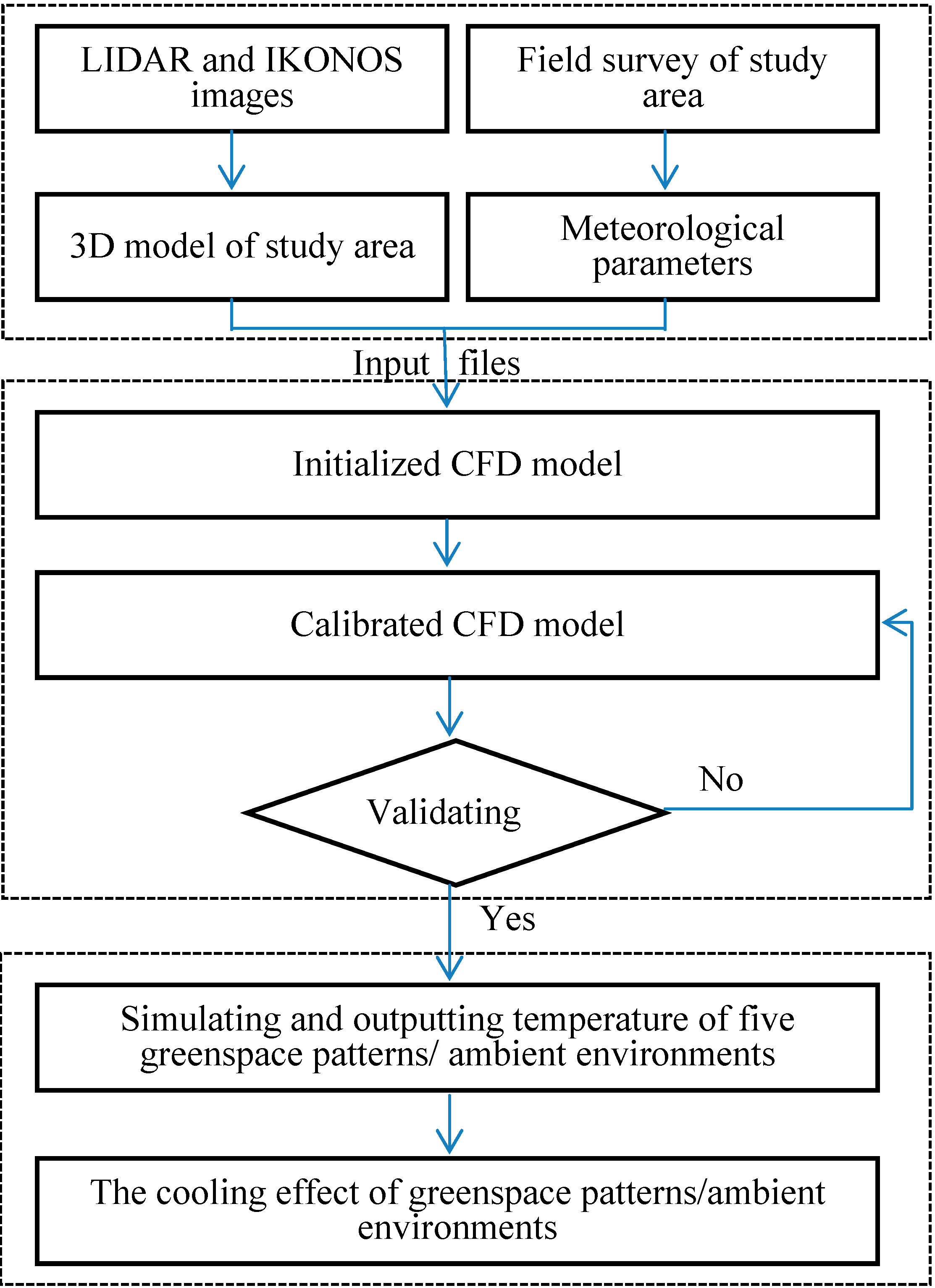
- (1)
- Constructing a 3D model of the study area based on LiDAR data and IKONOS images;
- (2)
- Initializing the CFD model by field survey and defining basic settings, including temperature at 1.5 m above ground: 299 K; wind speed (at 10 m above ground): 1.6 m/s; wind direction: south to north; RH: 84%; roughness length in 10 m: 0.1; total simulation: 24 h;
- (3)
- Calibrating the CFD model: comparing simulated temperature with measured temperature and adjusting the inputted parameters to make the simulation stable and the errors reduce;
- (4)
- Outputting the simulated temperature: simulating the temperatures of different scenarios based on systematic verification and reliability analysis of the ENVI-met model after inputting the two main files (Figure 1).
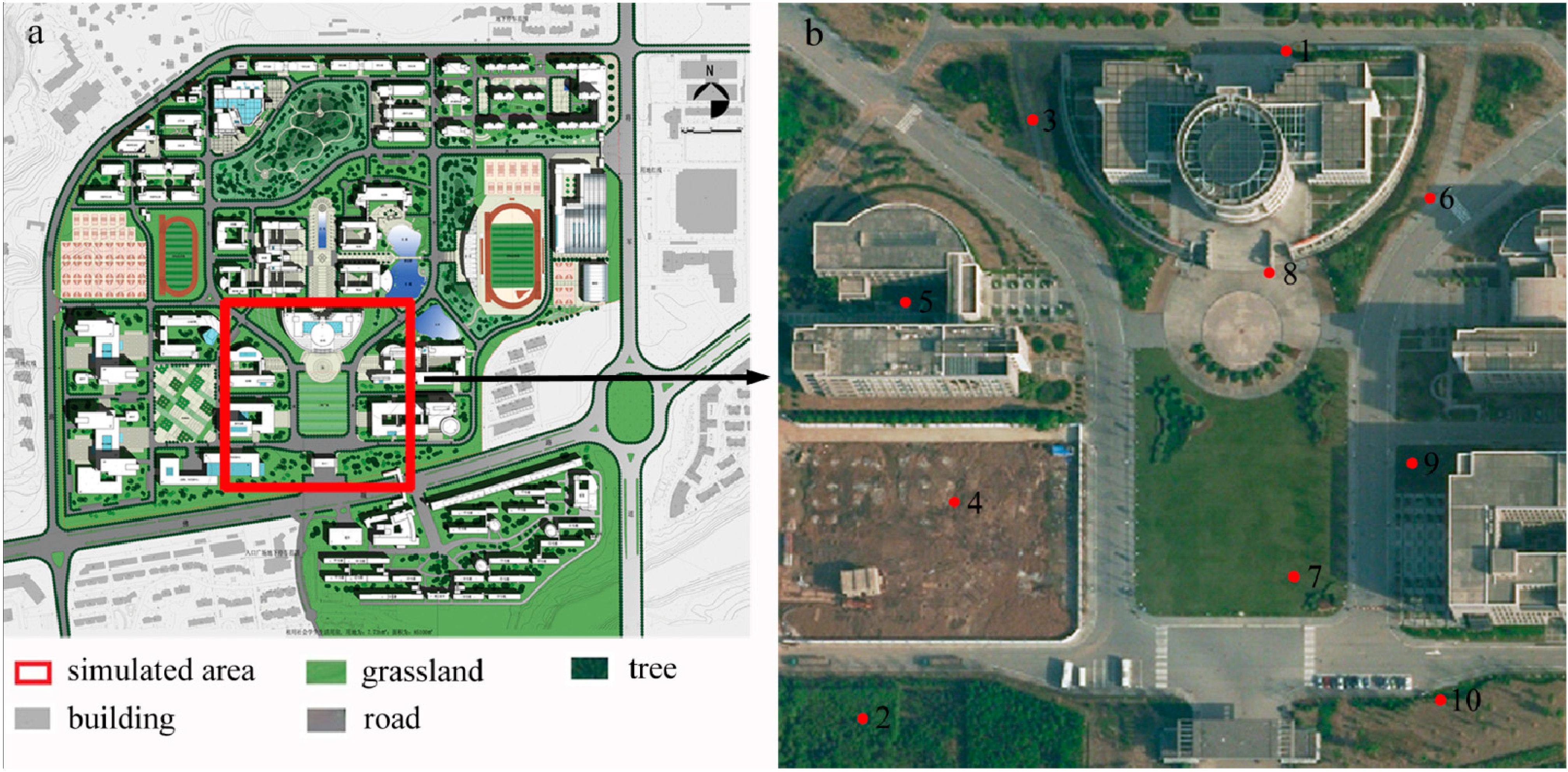
2.1. The Study Area and Data to Calibrate the CFD Model

2.2. Reconstructing 3D Urban Model and Field Survey

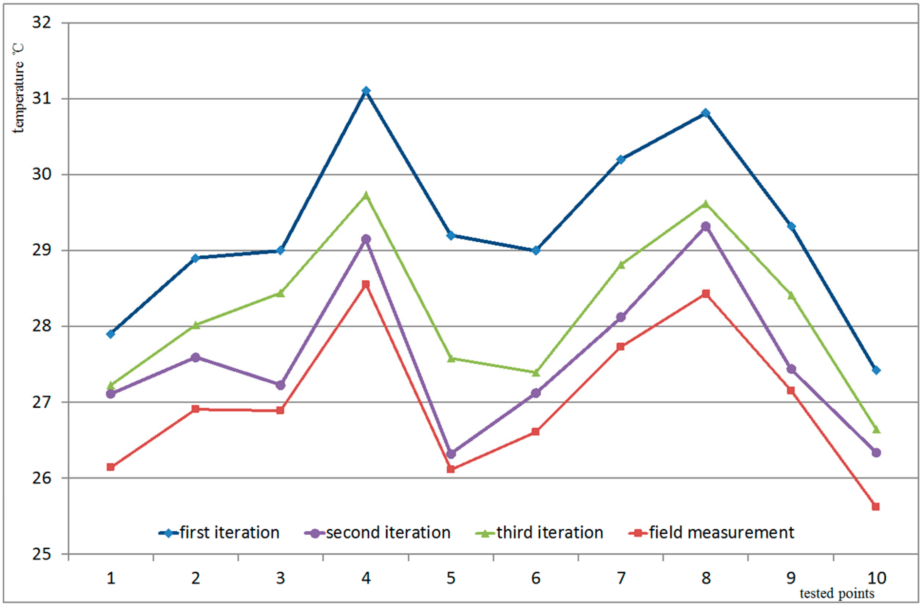
2.3. Calibrating CFD Model
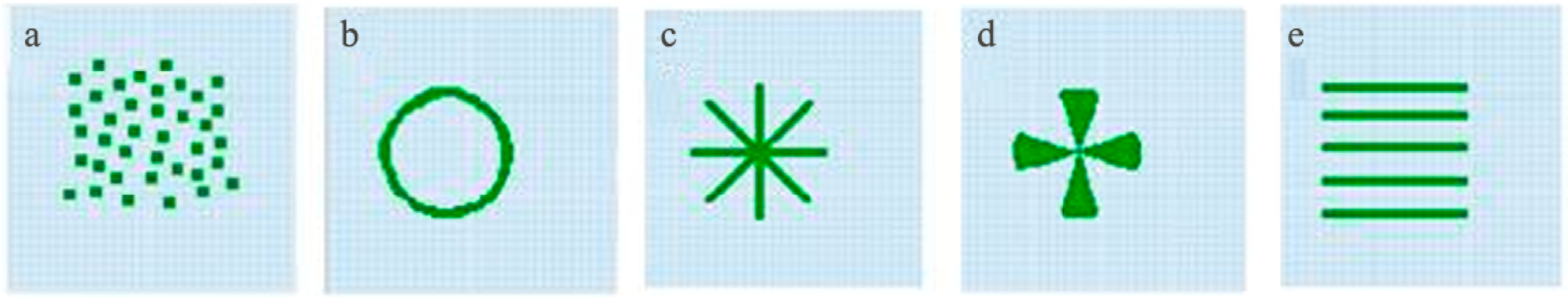
2.4. Five Models of Greenspace Pattern


| Case | Underlying type | Vegetation type | Vegetation Height (m) | Vegetation area (km2) | Total area (km2) | Obstruction situation |
|---|---|---|---|---|---|---|
| a | soil | tree | 5 | 0.08 | 0.64 | no |
| b | soil | grass | 0.2 | 0.04 | 0.64 | no |
| c | soil | tree | 5 | 0.04 | 0.64 | no |
| d | soil | tree | 5 | 0.04 | 0.64 | buildings |
| e | grass | tree | 5 | 0.04 | 0.64 | no |
3. Results
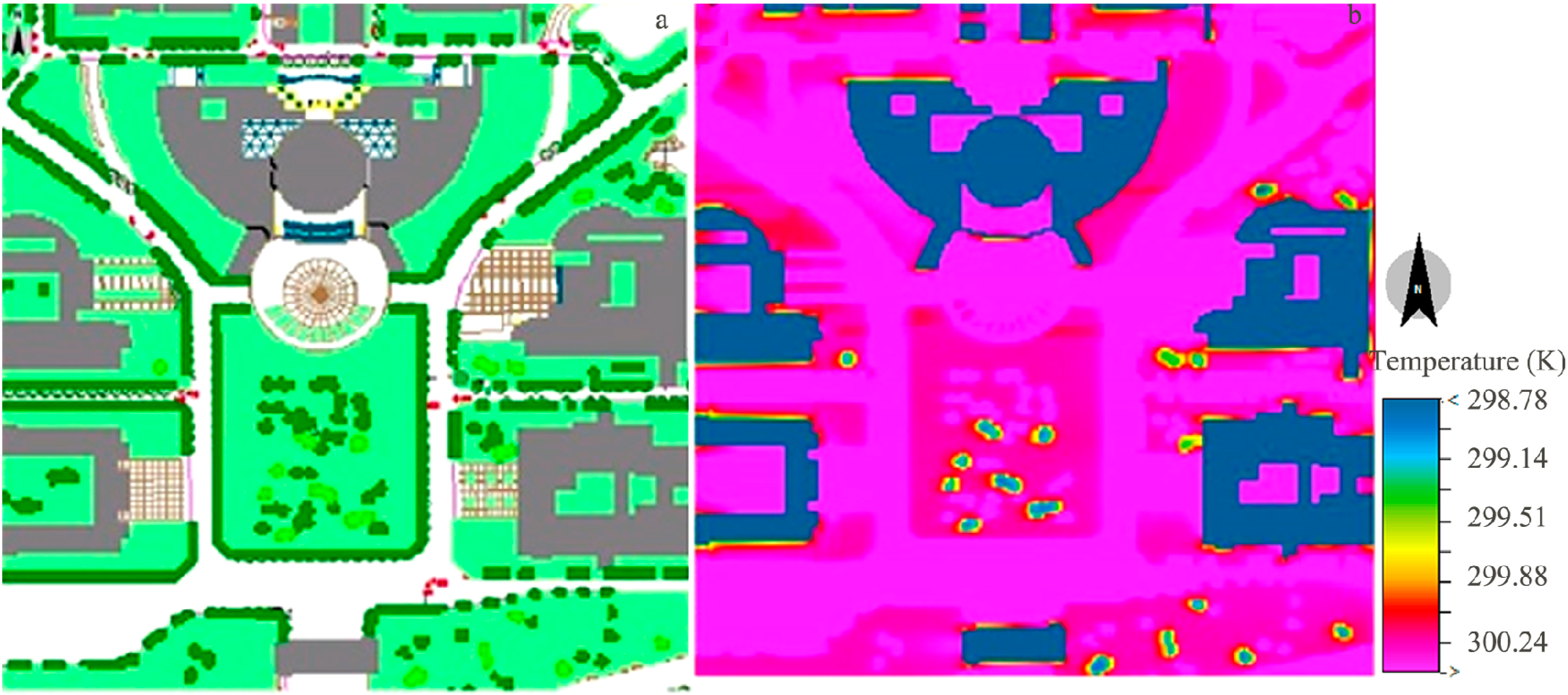
3.1. Simulated Temperature of Five Types of Greenspace Patterns
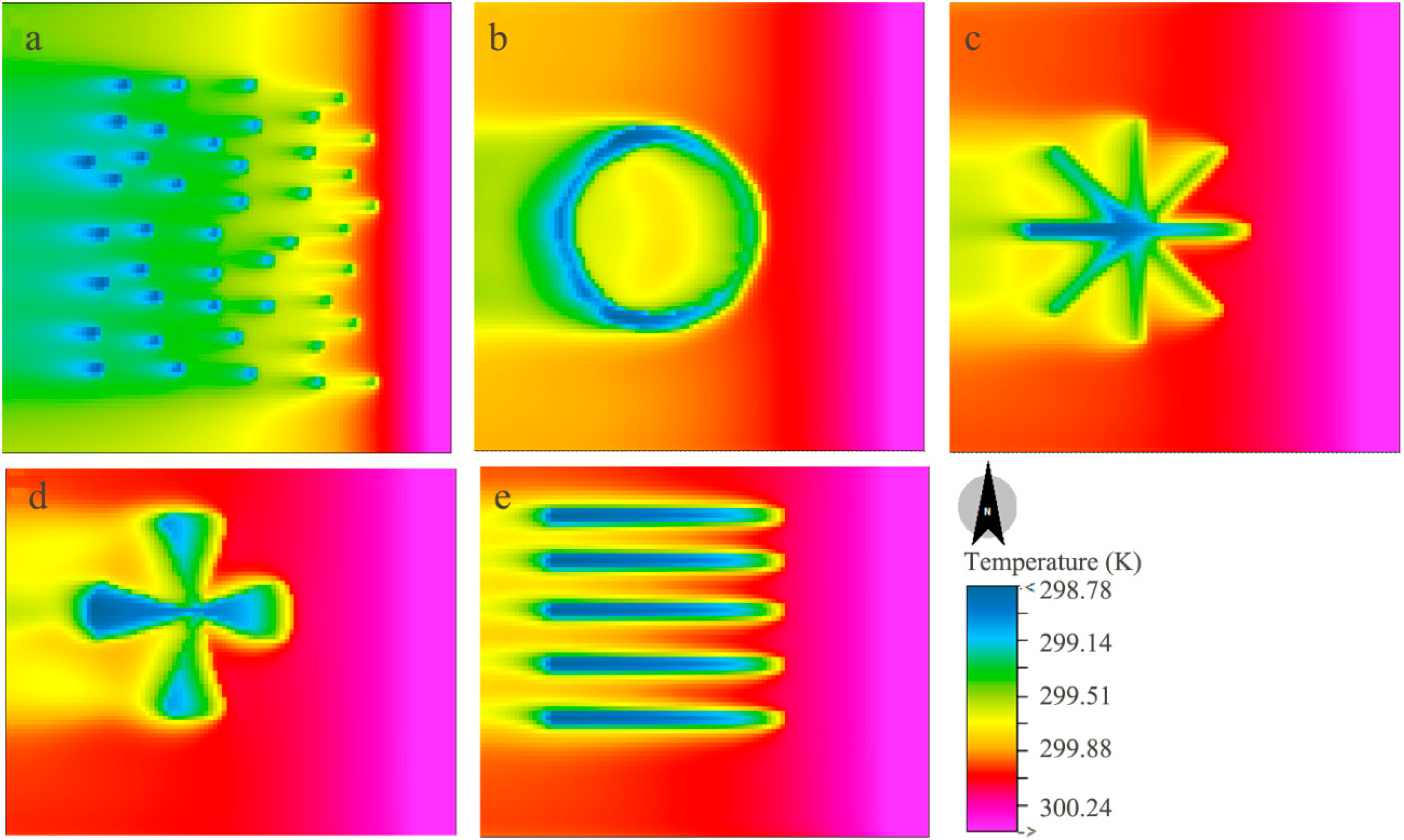
| Pattern | Average temperature (K) | Low temperature area (%) | High temperature area (%) | Median temperature area (%) |
|---|---|---|---|---|
| Dotted pattern | 299.991 | 0 | 26.45 | 73.55 |
| Radial pattern | 299.509 | 2.79 | 21.98 | 75.23 |
| Circular pattern | 299.740 | 0.96 | 25.25 | 73.79 |
| Zonal pattern | 298.768 | 6.09 | 25.55 | 68.36 |
| Wedge pattern | 299.491 | 3.38 | 17.86 | 78.76 |
3.2. Impact of Ambient Environment on Mitigating Effect of Greenspace Pattern
4. Discussions
4.1. The Importance of Model Calibration
4.2. The Cooling Effect of Greenspace Pattern on UHI
4.3. The Influences of Ambient Environment on the Cooling Effect of the Greenspace Pattern
5. Conclusions
Acknowledgments
Author Contributions
Conflicts of Interest
References
- Landsberg, H.E. The Urban Climate; Academic Press: New York, NY, USA, 1981. [Google Scholar]
- Sarrat, C.; Lemonsu, A.; Masson, V.; Guedalia, D. Impact of urban heat island on regional atmospheric pollution. Atmos. Environ. 2006, 40, 1743–1758. [Google Scholar]
- Bowler, D.E.; Buyung-Ali, L.; Knight, T.M.; Pullin, A.S. Urban greening to cool towns and cities: A systematic review of the empirical evidence. Landsc. Urban Plan. 2010, 97, 147–155. [Google Scholar]
- Coutts, A.M.; Daly, E.; Beringer, J.; Tapper, N.J. Assessing practical measures to reduce urban heat: Green and cool roofs. Build. Environ. 2013, 70, 266–276. [Google Scholar]
- Gill, S.; Handley, J.; Ennos, A.; Pauleit, S. Adapting cities for climate change: The role of the green infrastructure. Built Environ. 2007, 3, 115–133. [Google Scholar]
- Gill, S.E.; Handley, J.F.; Ennos, A.R.; Pauleit, S.; Theuray, N.; Lindley, S.J. Characterising the urban environment of UK cities and towns: A template for landscape planning. Landsc. Urban Plan. 2008, 87, 210–222. [Google Scholar]
- Chang, C.-R.; Li, M.-H.; Chang, S.-D. A preliminary study on the local cool-island intensity of Taipei city parks. Landsc. Urban Plan. 2007, 80, 386–395. [Google Scholar]
- Zoulia, I.; Santamouris, M.; Dimoudi, A. Monitoring the effect of urban green areas on the heat island in Athens. Environ. Monit. Assess. 2009, 156, 275–292. [Google Scholar] [PubMed]
- Nyuk, H.W.; Puay, Y.T.; Yu, C. Study of thermal performance of extensive rooftop greenery systems in the tropical climate. Build. Environ. 2007, 42, 25–54. [Google Scholar]
- Skelhorn, C.; Lindley, S.; Levermore, G. The impact of vegetation types on air and surface temperatures in a temperate city: A fine scale assessment in Manchester, UK. Landsc. Urban Plan. 2014, 121, 129–140. [Google Scholar]
- Yilmaz, S.; Toy, S.; Irmak, M.A.; Yilmaz, H. Determination of climatic differences in three different land uses in the city of Erzurum, Turkey. Build. Environ. 2007, 42, 1604–1612. [Google Scholar]
- Lehmann, I.; Mathey, J.; Rößler, S.; Bräuer, A.; Goldberg, V. Urban vegetation structure types as a methodological approach for identifying ecosystem services—Application to the analysis of micro-climatic effects. Ecol. Indicat. 2014, 42, 58–72. [Google Scholar]
- Li, X.; Zhou, W.; Ouyang, Z.; Xu, W.; Zheng, H. Spatial pattern of greenspace affects land surface temperature: Evidence from the heavily urbanized Beijing metropolitan area, China. Landsc. Ecol. 2012, 27, 887–898. [Google Scholar]
- Weng, Q.; Lu, D.; Schubring, J. Estimation of land surface temperature-vegetation abundance relationship for urban heat island studies. Rem. Sens. Environ. 2004, 89, 467–483. [Google Scholar]
- Zhou, W.; Huang, G.; Cadenasso, M.L. Does spatial configuration matter? Understanding the effects of land cover pattern on land surface temperature in urban landscapes. Landsc. Urban Plan. 2011, 102, 54–63. [Google Scholar]
- Su, W.; Yang, G.; Chen, S.; Yang, Y. Measuring the Pattern of High Temperature Areas in Urban Greenery of Nanjing City, China. Int. J. Environ. Res. Publ. Health. 2012, 9, 2922–2935. [Google Scholar]
- Takebayashi, H.; Moriyama, M. Surface heat budget on green roof and high reflection roof for mitigation of urban heat island. Build. Environ. 2007, 42, 2971–2979. [Google Scholar]
- Wong, M.S.; Nichol, J.E. Spatial variability of frontal area index and its relationship with urban heat island intensity. Int. J. Rem. Sens. 2012, 34, 885–896. [Google Scholar]
- Su, W.; Gu, C.; Yang, G. Assessing the impact of land use/land cover on urban heat island pattern in Nanjing City, China. J. Urban Plan. Dev. 2010, 136, 365–372. [Google Scholar]
- Mirzaei, P.A.; Haghighat, F. Approaches to study Urban Heat Island—Abilities and limitations. Build. Environ. 2010, 45, 2192–2201. [Google Scholar]
- Lee, S.-H.; Lee, K.-S.; Jin, W.-C.; Song, H.-K. Effect of an urban park on air temperature differences in a central business district area. Landsc. Ecol. Eng. 2009, 5, 183–191. [Google Scholar]
- Wong, N.H.; Yu, C. Study of green areas and urban heat island in a tropical city. Habitat Int. 2005, 29, 547–558. [Google Scholar]
- Liu, L.; Zhang, Y. Urban heat island analysis using the Landsat TM data and ASTER data: A case study in Hong Kong. Rem. Sens. 2011, 3, 1535–1552. [Google Scholar]
- Asawa, T.; Hoyano, A.; Nakaohkubo, K. Thermal design tool for outdoor spaces based on heat balance simulation using a 3D-CAD system. Build. Environ. 2008, 43, 2112–2123. [Google Scholar]
- Ferreira, R.A.C.; Silva Zacarin, E.C.M.; Malaspina, O.; Bueno, O.C.; Tomotake, M.E.M.; Pereira, A.M. Cellular responses in the Malpighian tubules of Scaptotrigona postica (Latreille, 1807) exposed to low doses of fipronil and boric acid. Micron 2013, 46, 57–65. [Google Scholar] [PubMed]
- Ashie, Y.; Kono, T. Urban-scale CFD analysis in support of a climate-sensitive design for the Tokyo Bay area. Int. J. Climatol. 2011, 31, 174–188. [Google Scholar]
- Melnyk, L.; Bernard, C.; Morgan, J. Detection of toxicants on building surfaces following a chemical attack. In Proceeding of the ACS Meeting, New York, NY, USA, 7–11 September 2003.
- Takahashi, K.; Yoshida, H.; Tanaka, Y.; Aotake, N.; Wang, F. Measurement of thermal environment in Kyoto city and its prediction by CFD simulation. Energ. Build. 2004, 36, 771–779. [Google Scholar]
- Weng, Q. Thermal infrared remote sensing for urban climate and environmental studies: Methods, applications, and trends. ISPRS J. Photogramm. Rem. Sens. 2009, 64, 335–344. [Google Scholar]
- Hedger, R.D.; Olsen, N.R.; Malthus, T.J.; Atkinson, P.M. Coupling remote sensing with computational fluid dynamics modelling to estimate lake chlorophyll-a concentration. Rem. Sens. Environ. 2002, 79, 116–122. [Google Scholar]
- Bruse, M. ENVI-met bulletin board. Available online: http://www.envi-met.com (accessed on 17 March 2009).
- Bruse, M.; Fleer, H. Simulating surface-plant-air interactions inside urban environents with a three dimensional numerical model. Environ. Model. Software 1998, 13, 373–384. [Google Scholar]
- Huttner, S.; Bruse, M.; Dostal, P. Using ENVI-met to simulate the impact of global warming on the microclimate in Central European Cities. In 5th Japanese-German Meeting on Urban Climatology; Meteorological Institute, Albert-Ludwigs-University: Freiburg, Germangy, 2008; pp. 307–312. [Google Scholar]
- Maggiotto, G.; Buccolieri, R.; Santo, M.A.; Leo, L.S.; di Sabatino, S. Validation of temperature-perturbation and CFD-based modelling for the prediction of the thermal urban environment: The Lecce (IT) case study. Environ. Model. Softw. 2014, 60, 69–83. [Google Scholar]
- Cheng, L.; Gong, J.; Li, M.; Liu, Y. 3D Building Model Reconstruction from Multi-view Aerial Imagery and Lidar Data. Photogramm. Eng. Rem. Sens. 2011, 77, 125–139. [Google Scholar]
- Satari, M.; Samadzadegan, F.; Azizi, A.; Maas, H.G. A Multi-Resolution Hybrid Approach for Building Model Reconstruction from Lidar Data. Photogramm. Rec. 2012, 27, 330–359. [Google Scholar]
- Chen, S.; Jim, C.Y. Quantitative assessment of the treescape and cityscape of Nanjing, China. Landsc. Ecol. 2003, 18, 395–412. [Google Scholar]
- Awrangjeb, M.; Zhang, C.; Fraser, C.S. Automatic extraction of building roofs using LiDAR data and multispectral imagery. ISPRS J. Photogramm. Rem. Sens. 2013, 83, 1–18. [Google Scholar]
- Cheng, L.; Tong, L.; Chen, Y.; Zhang, W.; Shan, J.; Liu, Y.; Li, M. Integration of LiDAR data and optical multi-view images for 3D reconstruction of building roofs. Optic Laser Eng. 2013, 51, 493–502. [Google Scholar]
- Uzar, M.; Yastikli, N. Automatic building extraction using LiDAR and aerial photographs. Bol. Ciênc. Geod. 2013, 19, 153–171. [Google Scholar]
- Chen, L.; Zhao, S.; Han, W.; Li, Y. Building detection in an urban area using lidar data and QuickBird imagery. Int. J. Rem. Sens. 2012, 33, 5135–5148. [Google Scholar]
- Kim, J.; Muller, J.-P. Tree and building detection in dense urban environments using automated processing of IKONOS image and LiDAR data. Int. J. Rem. Sens. 2011, 32, 2245–2273. [Google Scholar]
- Chen, Q.; Gong, P.; Baldocchi, D.; Xie, G. Filtering Airborne Laser Scanning Data with Morphological Methods. Photogramm. Eng. Rem. Sens. 2007, 73, 175–185. [Google Scholar]
- Sohn, G.; Dowman, I. Data fusion of high-resolution satellite imagery and LiDAR data for automatic building extraction. ISPRS J. Photogramm. Rem. Sens. 2007, 62, 43–63. [Google Scholar]
- Vosselman, G.; Dijkman, S. 3D building model reconstruction from point clouds and ground plans. Int. Arch. Photogramm. Rem. Sens. Spat. Inform. Sci. 2001, 34, 37–44. [Google Scholar]
- Turner, M.G. Spatial and temporal analysis of landscape patterns. Landsc. Ecol. 1990, 4, 21–30. [Google Scholar]
- Poudyal, N.C.; Hodges, D.G.; Tonn, B.; Cho, S.H. Valuing diversity and spatial pattern of open space plots in urban neighborhoods. For. Pol. Econ. 2009, 11, 194–201. [Google Scholar]
- Emmanuel, R.; Fernando, H. Urban heat islands in humid and arid climates: Role of urban form and thermal properties in Colombo, Sri Lanka and Phoenix, USA. Clim. Res. 2007, 34, 241–251. [Google Scholar]
- Wong, N.H.; Kardinal Jusuf, S.; Aung La Win, A.; Kyaw Thu, H.; Syatia Negara, T.; Xuchao, W. Environmental study of the impact of greenery in an institutional campus in the tropics. Build. Environ. 2007, 42, 2949–2970. [Google Scholar]
- Murakami, S. Environmental design of outdoor climate based on CFD. Fluid Dynam. Res. 2006, 38, 108–126. [Google Scholar]
- Li, K.; Yu, Z. Comparative and combinative study of urban heat island in Wuhan City with remote sensing and CFD simulation. Sensors 2008, 8, 6692–6703. [Google Scholar]
- Bonan, G.B. The microclimates of a suburban Colorado (USA) landscape and implications for planning and design. Landsc. Urban Plan. 2000, 49, 97–114. [Google Scholar]
- Shashua-Bar, L.; Pearlmutter, D.; Erell, E. The cooling efficiency of urban landscape strategies in a hot dry climate. Landsc. Urban Plan. 2009, 92, 179–186. [Google Scholar]
- Erell, E.; Williamson, T. Simulating air temperature in an urban street canyon in all weather conditions using measured data at a reference meteorological station. Int. J. Climatol. 2006, 26, 1671–1694. [Google Scholar]
© 2014 by the authors; licensee MDPI, Basel, Switzerland. This article is an open access article distributed under the terms and conditions of the Creative Commons Attribution license (http://creativecommons.org/licenses/by/4.0/).
Share and Cite
Su, W.; Zhang, Y.; Yang, Y.; Ye, G. Examining the Impact of Greenspace Patterns on Land Surface Temperature by Coupling LiDAR Data with a CFD Model. Sustainability 2014, 6, 6799-6814. https://doi.org/10.3390/su6106799
Su W, Zhang Y, Yang Y, Ye G. Examining the Impact of Greenspace Patterns on Land Surface Temperature by Coupling LiDAR Data with a CFD Model. Sustainability. 2014; 6(10):6799-6814. https://doi.org/10.3390/su6106799
Chicago/Turabian StyleSu, Weizhong, Yong Zhang, Yingbao Yang, and Gaobin Ye. 2014. "Examining the Impact of Greenspace Patterns on Land Surface Temperature by Coupling LiDAR Data with a CFD Model" Sustainability 6, no. 10: 6799-6814. https://doi.org/10.3390/su6106799
APA StyleSu, W., Zhang, Y., Yang, Y., & Ye, G. (2014). Examining the Impact of Greenspace Patterns on Land Surface Temperature by Coupling LiDAR Data with a CFD Model. Sustainability, 6(10), 6799-6814. https://doi.org/10.3390/su6106799