A National-Scale Method for Estimating the Rainfall Erosivity Factor (R) from Daily Rainfall Totals in Mexico

Abstract

Rainfall erosivity is a key driver of soil erosion and a fundamental input to the Revised Universal Soil Loss Equation (RUSLE). Its direct estimation, however, requires high-temporal-resolution rainfall records to compute the storm erosivity index, EI₃₀, which are available at relatively few locations. This limitation constrains erosion assessment and conservation planning in many regions of Mexico. This study develops and evaluates an empirical methodology to estimate the annual rainfall erosivity factor, R, from more widely available daily rainfall totals. A total of 170,796 storm events recorded at 432 automatic weather stations were analyzed to derive four-parameter nonlinear relationships between daily rainfall depth and storm erosivity. The resulting equations provide site-specific transfer functions that were subsequently applied to 2124 climatological stations for the common period 1965–2006. In addition, a station-based quantitative comparison was conducted at the Cerro Catedral Automatic Weather Station, where a reference annual erosivity series was derived directly from 10 min rainfall records. For this case study, the proposed methodology reproduced the reference annual erosivity series more closely than the regional equations of Cortes, yielding a substantially lower standard error of fit (SEF = 347 MJ·mm·ha⁻¹·h⁻¹·yr⁻¹ versus 1455.77 MJ·mm·ha⁻¹·h⁻¹·yr⁻¹). At the national scale, the resulting erosivity patterns were spatially coherent with the major rainfall gradients of Mexico and supported by a substantially larger observational dataset than previous national formulations. By enabling national-scale erosivity estimation from standard daily rainfall data, the methodology expands the spatial applicability of RUSLE and provides a practical basis for soil erosion assessment, sediment-yield studies, and land and water conservation planning under current and future hydroclimatic pressures.

1. Introduction

Mexico covers approximately 1.964 million km² and is characterized predominantly by dry climates. This climatic pattern is mainly controlled by the subtropical high-pressure belt, located roughly between 15° N and 30° N, together with the orographic barriers formed by the Sierra Madre Occidental and Sierra Madre Oriental mountain ranges. Aridity is particularly pronounced in northern and northwestern Mexico, where the influence of the Intertropical Convergence Zone is comparatively weak. Mean annual precipitation is approximately 750 mm, although its spatial distribution is highly uneven, ranging from less than 500 mm in the north and northwest to more than 2000 mm in the south and southeast. In addition, about 68% of annual rainfall occurs between June and September [1], intensifying both seasonal water scarcity and the risks of flooding and soil erosion. These pressures are expected to become more severe under climate variability and climate change, especially in regions where changes in rainfall regime, land cover, and storm organization may alter erosive forcing over time [2,3].

Agriculture remains a strategic sector in Mexico, contributing 3.4% of the gross domestic product and employing 12.5% of the economically active population. Approximately 21.8 million hectares are used for agricultural production across a wide range of soil types [1]. Because agricultural productivity depends directly on soil quality, water availability, and adequate agronomic management, including nutrient and fertilizer use, soil conservation is essential not only for sustaining food production but also for preserving the long-term environmental and economic sustainability of many regions of the country. In this context, reliable estimation of rainfall-driven soil erosion is fundamental for land-use planning, watershed protection, and the design of conservation practices.

Soil, defined as the outermost layer of the Earth’s crust, consists of unconsolidated and fragmented material formed through the combined action of climate, organisms, relief, parent material, and time, following the classical soil-formation framework associated with Dokuchaev [4] and later formalized by Jenny [5]. Although erosion and sedimentation are natural geomorphic processes [6], human activities have accelerated them far beyond their natural rates [7]. When soil erosion exceeds the rate of soil formation, progressive degradation occurs, generally because of inadequate land use, poor management practices, and the action of intense rainfall events [8]. In this sense, soil loss is not only an environmental problem but also a clear indicator of unsustainable territorial development, because it reduces land productivity, weakens ecosystem functions, and increases the vulnerability of rural and urban systems.

The consequences of soil erosion are far-reaching. They include nutrient depletion, declining crop yields, and deterioration of soil structure, as well as increased sediment transport by rivers. Excess sediment can substantially reduce the useful storage capacity of reservoirs and hydroelectric facilities, while also increasing the turbidity of coastal waters and altering aquatic habitats and fisheries [7,8]. These effects propagate across multiple sectors and spatial scales, generating economic losses, environmental degradation, and growing pressure on water and land resources. From a sustainability perspective, continued soil loss undermines the capacity of regions to maintain agricultural production, conserve ecosystem services, and support resilient livelihoods over time. Recent reviews continue to emphasize that the erosivity factor remains one of the most critical and yet most data-demanding components of erosion assessment under the USLE/RUSLE framework [9].

Physical soil degradation includes water and wind erosion, structural deterioration, and processes such as sealing, crusting, and plow-pan formation [10,11]. Among these processes, water erosion is particularly important in many parts of Mexico because of the marked seasonality and intensity of rainfall [12,13,14]. It may occur in different forms and levels of severity depending on rainfall intensity, soil properties, topography, and the degree of surface protection [15,16,17]. Water erosion results from two main physical processes: the impact of raindrops on the soil surface and the subsequent generation of surface runoff. The process begins when raindrops strike the ground with sufficient energy to detach particles of unconsolidated material, producing splash erosion [7]. This is followed by sheet erosion, in which thin and relatively uniform layers of soil are removed. Under more intense runoff conditions, rill erosion may develop, forming small channels typically 5 to 10 cm deep. Once rills appear, erosion rates may increase considerably because of higher flow velocities. The most severe form is gully erosion, characterized by the development of deep and wide channels or ravines that may reach several meters in width and depth. Recent applications in Mexico confirm that these processes continue to motivate the use and adjustment of USLE/RUSLE-type approaches under local conditions [18,19].

Given the environmental, social, and economic implications of soil degradation, it is essential to identify areas with potential erosion risk and to quantify present and future soil losses in order to design and implement effective mitigation measures. This need is especially acute in regions where soil degradation threatens agricultural productivity, water security, and the long-term sustainability of local development. A wide range of methods and equations for estimating soil loss has been reported in the literature. Among them, the Universal Soil Loss Equation (USLE), proposed by Wischmeier and Smith [15,20], remains one of the most widely used approaches for estimating annual soil loss caused by sheet and rill erosion. The reliability of this method depends largely on the appropriate representation of its main controlling factors: rainfall characteristics, soil properties, topography, land cover and management, and conservation practices.

Within the USLE/RUSLE framework, the rainfall erosivity factor R is one of the most influential variables in soil-loss estimation in many regions of the world [21,22,23]. Wischmeier and Smith [15] defined storm erosivity as the product of total storm kinetic energy (E) and the maximum 30 min rainfall intensity (I₃₀). The annual erosivity factor R is then obtained by summing the erosivity of all erosive storms within a given year. Because detailed pluviographic records are scarce, however, R is often estimated from statistical relationships with more readily available rainfall variables, such as mean annual rainfall [21] or mean monthly rainfall [24,25,26]. Several studies have shown, nevertheless, that daily rainfall records provide a more robust basis for estimating rainfall erosivity than coarser annual or monthly summaries [26,27,28,29,30]. Recent work has also shown that erosivity estimation remains an active field of methodological development, including empirical equations for data-scarce areas [2], broad national compilations of erosivity information [31], and comparative evaluations of alternative erosivity factors for watershed applications [32].

Internationally, daily rainfall-based erosivity estimation has been explored in a wide range of climatic settings. Examples include Mediterranean environments such as northeastern Spain [28], Atlantic climates such as Portugal [24], northern Europe [25], and large Asian river basins such as the Yangtze River basin [26]. At broader scales, continental assessments have highlighted both the importance of high-temporal-resolution rainfall records and the persistent need for transferable methodologies in data-scarce regions [33]. More recent studies confirm this continuing research interest. Dela Cruz et al. [2] developed an empirical equation for estimating the rainfall erosivity factor for application in soil-loss models in a data-scarce tropical setting, whereas Oliveira-Roza et al. [31] compiled a large national rainfall erosivity database for Brazil, underscoring the importance of spatially extensive datasets for conservation planning. Fofang et al. [3] examined landcover-rainfall interactions in the Lake Tana Basin and reported a rising erosivity signal in a changing environmental context, while Miao et al. [32] evaluated the performance of different rainfall and runoff erosivity factors in the Fu River Basin and showed that factor suitability may vary according to watershed conditions and modeling purpose. Compared with these studies, the Mexican case is particularly challenging because of its pronounced climatic gradients, strong convective seasonality, and the limited availability of long sub-daily rainfall series relative to the much denser network of stations with daily rainfall records.

In Mexico, the equations proposed by Cortés [34] are still commonly used to estimate R as a function of accumulated annual rainfall through linear regression models developed for predefined regions. One limitation of those regional equations is that they cover extensive areas and do not adequately represent the spatial and temporal variability of rainfall. Although more recent Mexican studies have applied or adjusted USLE/RUSLE formulations at local scales [18,19], a national-scale methodology that links storm-scale erosivity to daily rainfall totals remains lacking. Against this background, the objective of the present study is to develop a methodology for estimating the annual rainfall erosivity factor R from daily rainfall totals. The proposed approach is based on the analysis of 170,796 storm events recorded at 10 min intervals at 432 automatic weather stations (AWS). In practical terms, this contribution seeks to improve erosivity assessment in a country where accelerated soil loss already compromises regional sustainability by reducing long-term agricultural productivity, degrading hydrological regulation, increasing sedimentation in reservoirs and hydraulic infrastructure, and weakening the adaptive capacity of ecosystems and communities.

2. Materials and Methods

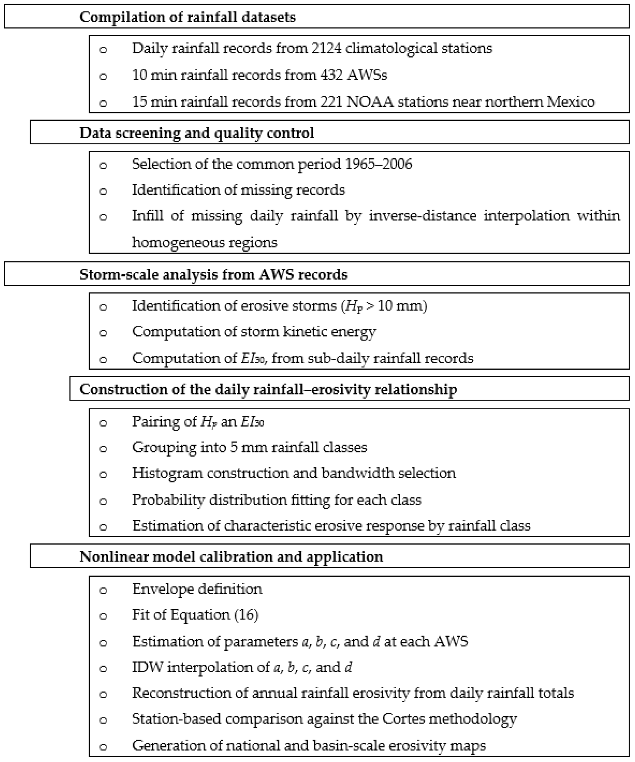
To derive the proposed relationship between daily rainfall totals and rainfall erosivity, the methodological framework was organized into four main components: characterization of the study area, assembly and screening of rainfall data, computation of storm erosivity within the USLE/RUSLE framework, and derivation of a predictive relationship between daily rainfall depth and storm erosivity. Because this procedure involves multiple datasets and sequential analytical steps, the overall workflow is summarized schematically in Figure 1.

The flow chart highlights how sub-daily records from automatic weather stations were used to calibrate the rainfall–erosivity relationship and how the resulting transfer functions were subsequently applied to the climatological network to reconstruct annual rainfall erosivity at the national scale.

2.1. Study Area

Mexico is located between 14°32′00″ and 32°43′00″ N latitude and between 86°42′00″ and 118°27′00″ W longitude. It is bordered by the United States to the north, Guatemala and Belize to the south, the Gulf of Mexico to the east, and the Pacific Ocean to the west.

To place the analysis in its national environmental context, soil degradation conditions across the country were first examined. According to the report Evaluación de la degradación del suelo causada por el hombre en la República Mexicana, 44.9% of the country’s soils were affected by some form of degradation in both natural ecosystems and managed lands [12]. Chemical degradation was the most widespread type, affecting 34.0 million hectares (17.8% of the national territory), followed by water erosion with 22.7 million hectares (11.9%), wind erosion with 18.1 million hectares (9.5%), and physical degradation with 10.8 million hectares (5.7%) [12]. By contrast, soils without apparent degradation accounted for 55.1% of the country, equivalent to 105.2 million hectares [12].

The causes of soil degradation in Mexico are diverse. Approximately 35% of the degraded area is associated with agricultural and livestock activities, each contributing about 17.5%, while 7.4% is linked to the loss of vegetation cover. The remainder is distributed among urbanization, overexploitation of vegetation, and industrial activities [12]. Water erosion is particularly relevant in mountainous regions, where 67% of national erosion by water occurs. These regions cover approximately 47% of the national territory, representing nearly 92 million hectares, of which about 14.8% exhibit topsoil loss and 1.9% show land deformation [12].

From the standpoint of rainfall erosivity, Mexico constitutes a highly heterogeneous setting. Pronounced contrasts in annual rainfall, strong seasonal concentration of precipitation, tropical cyclone influence along both coasts, and marked orographic effects create substantial regional differences in storm intensity and erosive forcing. These hydroclimatic contrasts provide a strong rationale for developing an erosivity methodology capable of preserving local and regional gradients rather than relying only on broad regional averages.

2.2. Data

The National Water Commission (CONAGUA) maintains daily rainfall records from approximately 4200 climatological stations distributed throughout Mexico [35]. After evaluating data quality and completeness, 2124 stations were selected for this study, specifically those with records covering the common period 1965–2006.

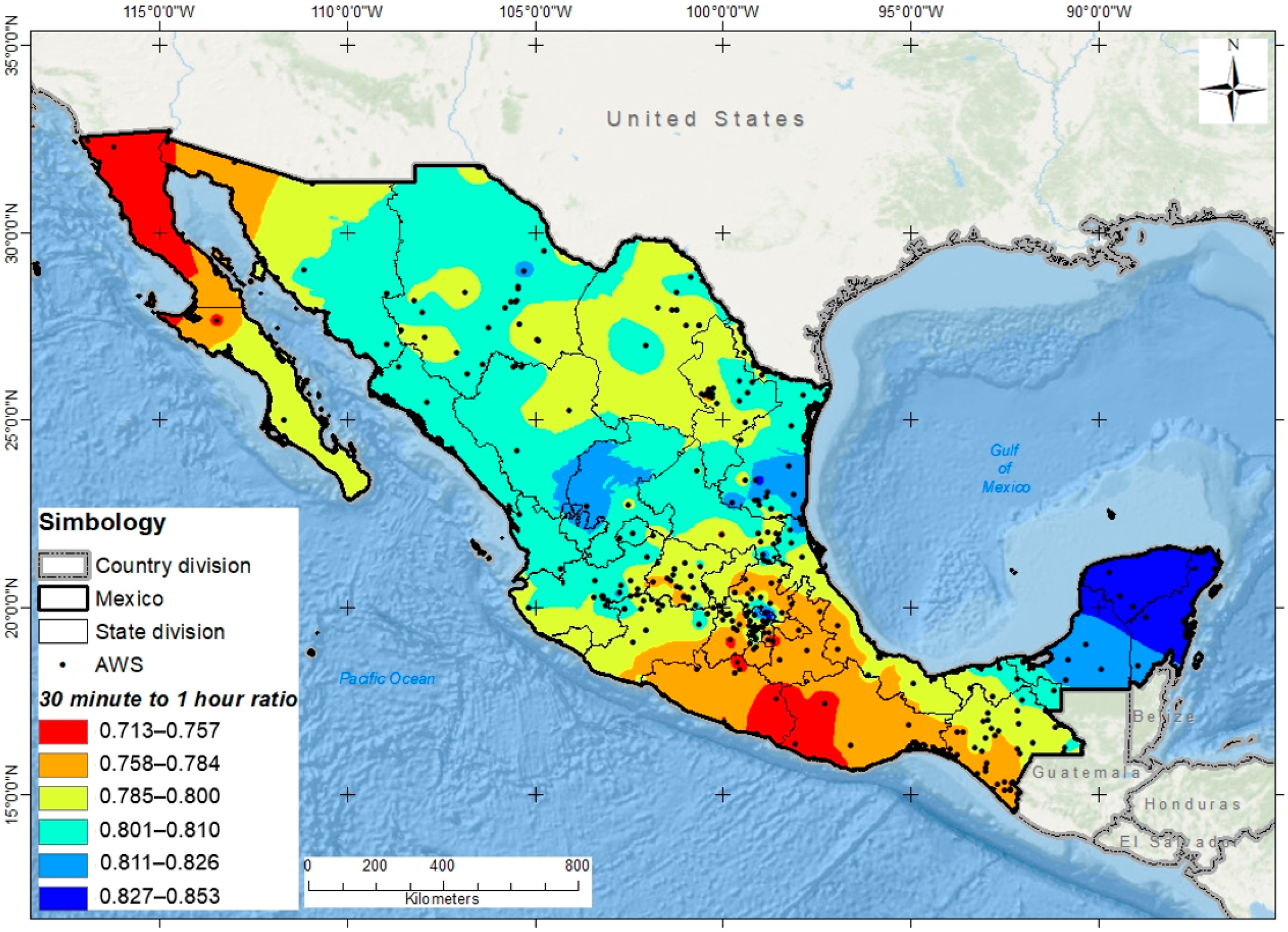
Because the proposed approach links daily rainfall information with storm-scale erosivity, special attention was given to data consistency and spatial comparability. Missing daily data were estimated by inverse-distance interpolation (IDW) [36]. Data transfer was carried out only between stations located within the same homogeneous region, defined on the basis of similar values of the 30-min to 1-h rainfall ratio. These ratios were derived from the analysis of storm records obtained from automatic weather stations (AWSs). The spatial pattern of this ratio is presented in Figure 2.

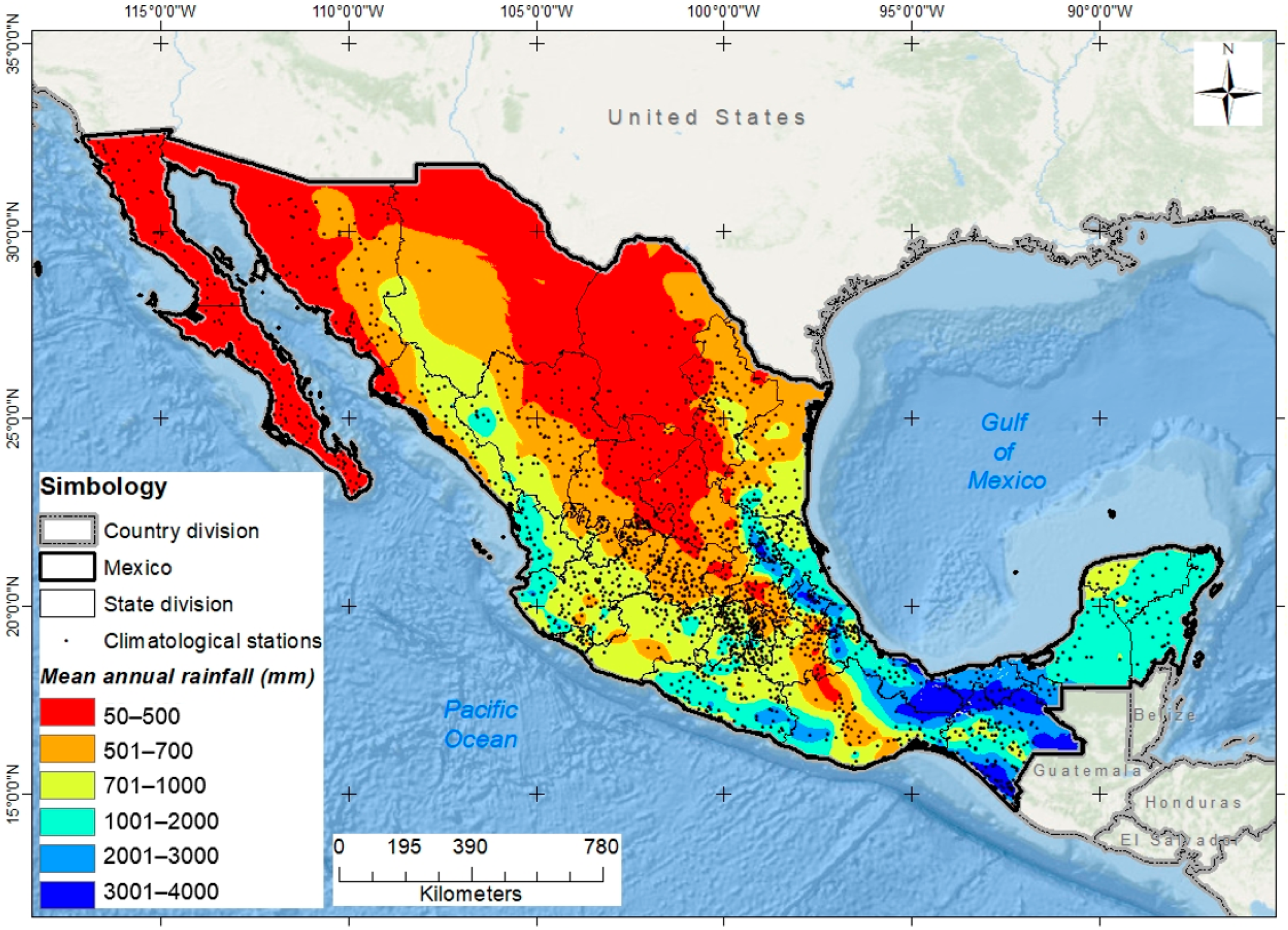
For reference, Figure 3 shows the spatial distribution of the 2124 climatological stations used in this study together with the corresponding mean annual rainfall for the period 1965–2006.

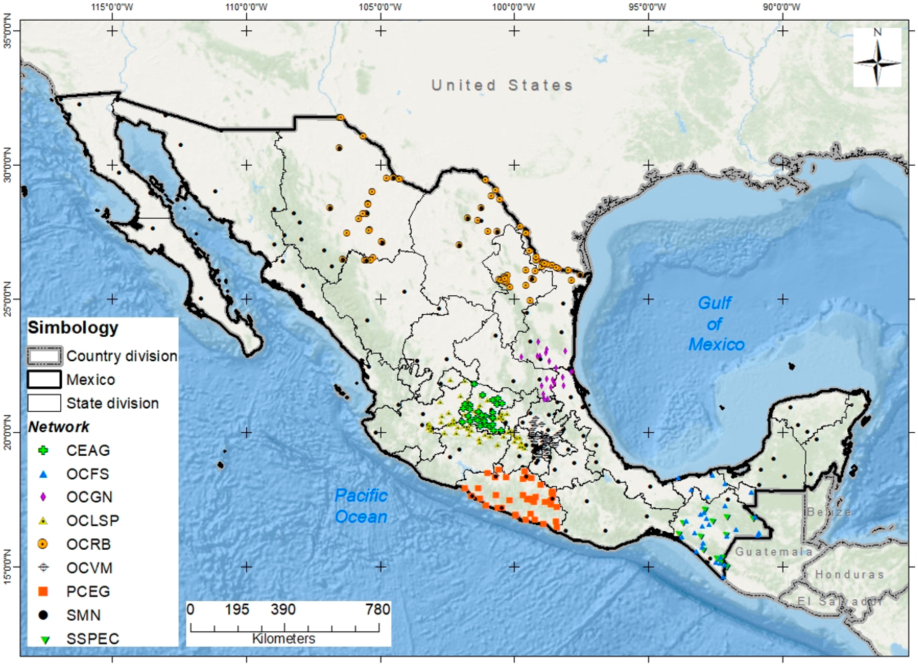
To characterize rainfall properties at durations shorter than 1 h, and particularly to determine the maximum 30 min intensity, 170,796 storms recorded at 432 Automatic Weather Stations (AWS) were analyzed. The distribution of these stations among the operational networks managed by CONAGUA is summarized in

Table 1. Operational networks of Automatic Weather Stations managed by CONAGUA.

Region	Network	Stations	Storms
1	Coordinación General del Servicio Meteorológico Nacional (SMN)	139	88,760
2	Organismo de Cuenca Aguas del Valles de México (OCVM)	25	2948
3	Organismo de Cuenca Golfo Norte (OCGN)	21	5504
4	Organismo de Cuenca Lerma–Santiago–Pacífico (OCLSP)	65	21,704
5	Organismo de Cuenca Río Bravo (OCRB)	71	19,294
6	Organismo de Cuenca Frontera Sur (OCFS)	28	4889
7	Comisión Estatal del Agua de Guanajuato (CEAG)	31	15,128
8	Protección Civil del Estado de Guerrero (PCEG)	39	7127
9	Secretaría de Seguridad Pública del Estado de Chiapas (SSPEC)	13	5442

.

In addition, to improve the characterization of rainfall timing and intensity in northern Mexico, 15 min rainfall records from 221 stations in the United States, located within 200 km of the Mexican border, were incorporated into the analysis [37]. The complete spatial distribution of the Mexican AWSs used in this study is presented in Figure 4. Only storms with rainfall depths greater than 10 mm were retained, because such events are more likely to generate significant soil erosion.

2.3. USLE/RUSLE Framework and Computation of Storm Erosivity

Once the rainfall database had been assembled, storm erosivity was quantified within the USLE/RUSLE framework. The Universal Soil Loss Equation (USLE) is an empirical model used to estimate soil loss caused by water erosion and is expressed as [15,20]:

$$A=R\hspace{0.33em}K\hspace{0.33em}LS\hspace{0.33em}C\hspace{0.33em}P$$

(1)

where A is the annual soil loss (t ha⁻¹), R is the rainfall erosivity factor, K is the soil erodibility factor, LS is the slope-length and slope-steepness factor, C is the cover-management factor, and P is the support-practice factor.

In 1996, the United States Department of Agriculture published an updated version of the model, known as the Revised Universal Soil Loss Equation (RUSLE), which introduced revised procedures for estimating the original USLE factors [22]. One of the main revisions concerned the computation of rainfall erosivity through storm kinetic energy.

To calculate storm erosivity, the kinetic energy associated with each rainfall increment must first be estimated. Rainfall kinetic energy depends primarily on raindrop size and terminal fall velocity, both of which are related to rainfall intensity. Wischmeier and Smith [38] adopted the following relationship between rainfall intensity and kinetic energy:

$$e_c=\left\{\begin{array}{c}916+331{log}_{10}\left(i\right), i\le 3in{h}^{-1}\\ 1074, i>3in{h}^{-1} \end{array}\right.$$

(2)

where $e_c$ is the rainfall kinetic energy per unit rainfall depth, expressed in ft·tonf·acre⁻¹·in⁻¹, and i is the rainfall intensity in in·h⁻¹ [38].

Brown and Foster [39] later proposed a modified expression calibrated with a larger dataset, which improves the prediction of kinetic energy at low rainfall intensities and approaches an asymptotic value at high intensities:

$$e_c=0.29\left[1-0.72 \mathit{exp}\left(-0.05i\right)\right]$$

(3)

where i is the rainfall intensity in mm·h⁻¹ and $e_c$ is expressed in MJ·mm⁻¹·ha⁻¹.

The total kinetic energy of storm j is obtained by summing the partial energies associated with each rainfall increment over the storm duration:

$$E_j={\sum }_{k=1}^m{e}_c\left(k\right)·\Delta Hp\left(k\right)$$

(4)

where $E_j$ is the total kinetic energy of storm j, m is the number of rainfall intervals in the storm, and $\Delta Hp\left(k\right)$ is the rainfall depth associated with interval k, expressed in mm.

The storm erosivity index is then computed as:

$${{EI}_{30,j}=E}_j{I}_{30,j}$$

(5)

or equivalently, by substituting Equation (3) into Equation (4)

$${EI}_{30,j}=\left\{{\sum }_{k=1}^{m}0.29\left[1-0.72 \mathit{exp}\left(-0.05i\left(k\right)\right)\right]·\Delta Hp\left(k\right)\right\}\cdot I_{30}$$

(6)

where ${EI}_{30,j}$ is the erosivity index of storm j, expressed in MJ·mm·ha⁻¹·h⁻¹ and $I_{30,j}$ is the maximum rainfall intensity over 30 min during storm j, expressed in mm·h⁻¹.

Finally, the annual rainfall erosivity factor for year y. is obtained by summing the erosivity values of all erosive storms occurring in that year:

$$R_y={\sum }_{j=1}^{N_y}{EI}_{30,j}$$

(7)

where $R_y$ is the annual rainfall erosivity factor for year y, N_y is the number of erosive storms recorded during that year.

2.4. Estimation of Storm Erosivity from Daily Rainfall Totals

After computing storm-scale erosivity values from sub-daily records, a five-step procedure was used to derive a predictive relationship between daily rainfall totals and storm erosivity.

• Step 1

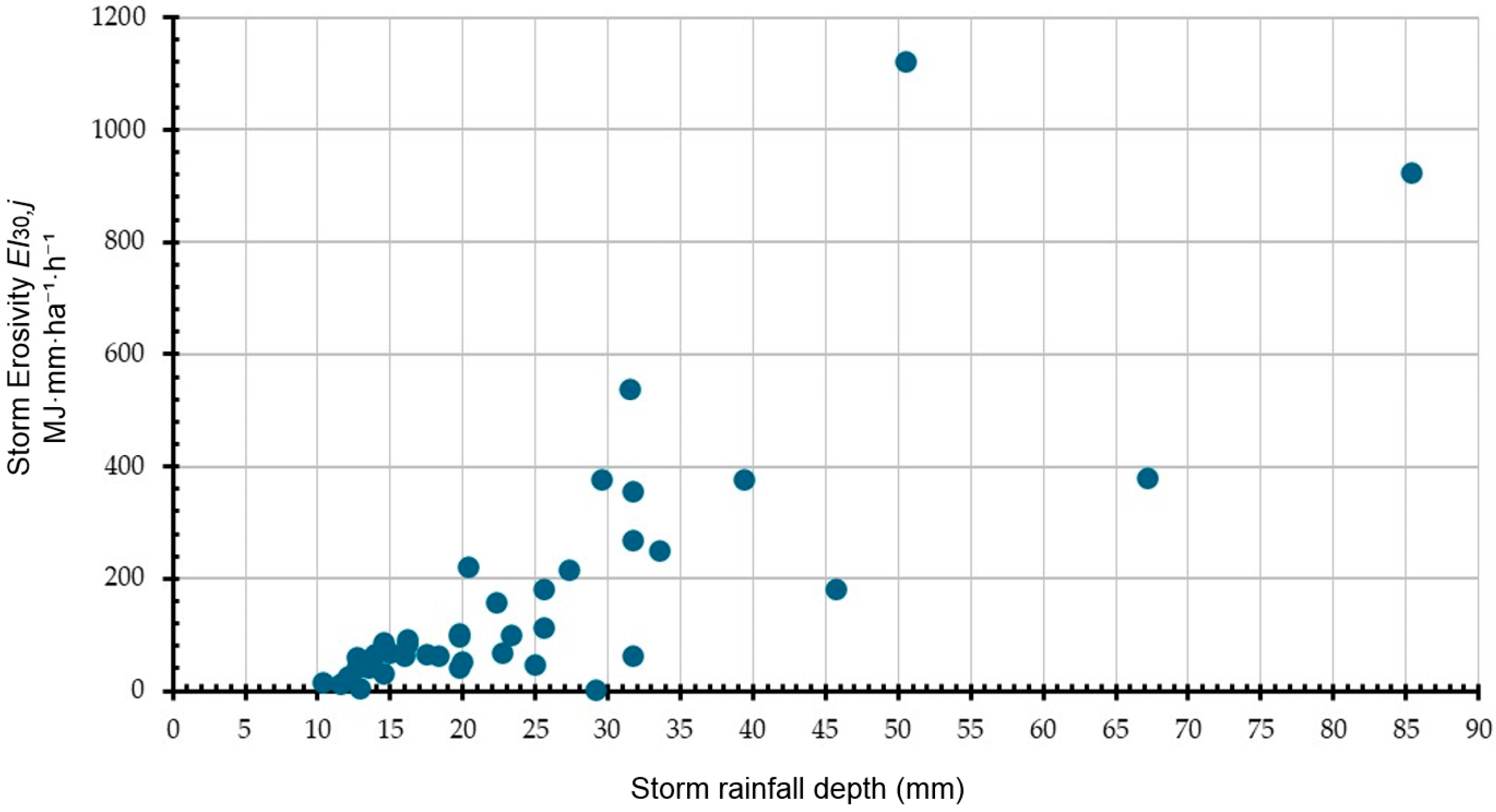
For each storm recorded at the AWSs, an ordered pair consisting of daily rainfall total (Storm rainfall depth) and its corresponding storm erosivity ${EI}_{30,j}$ was obtained from Equation (6). The resulting relationship is illustrated in Figure 5.

• Step 2

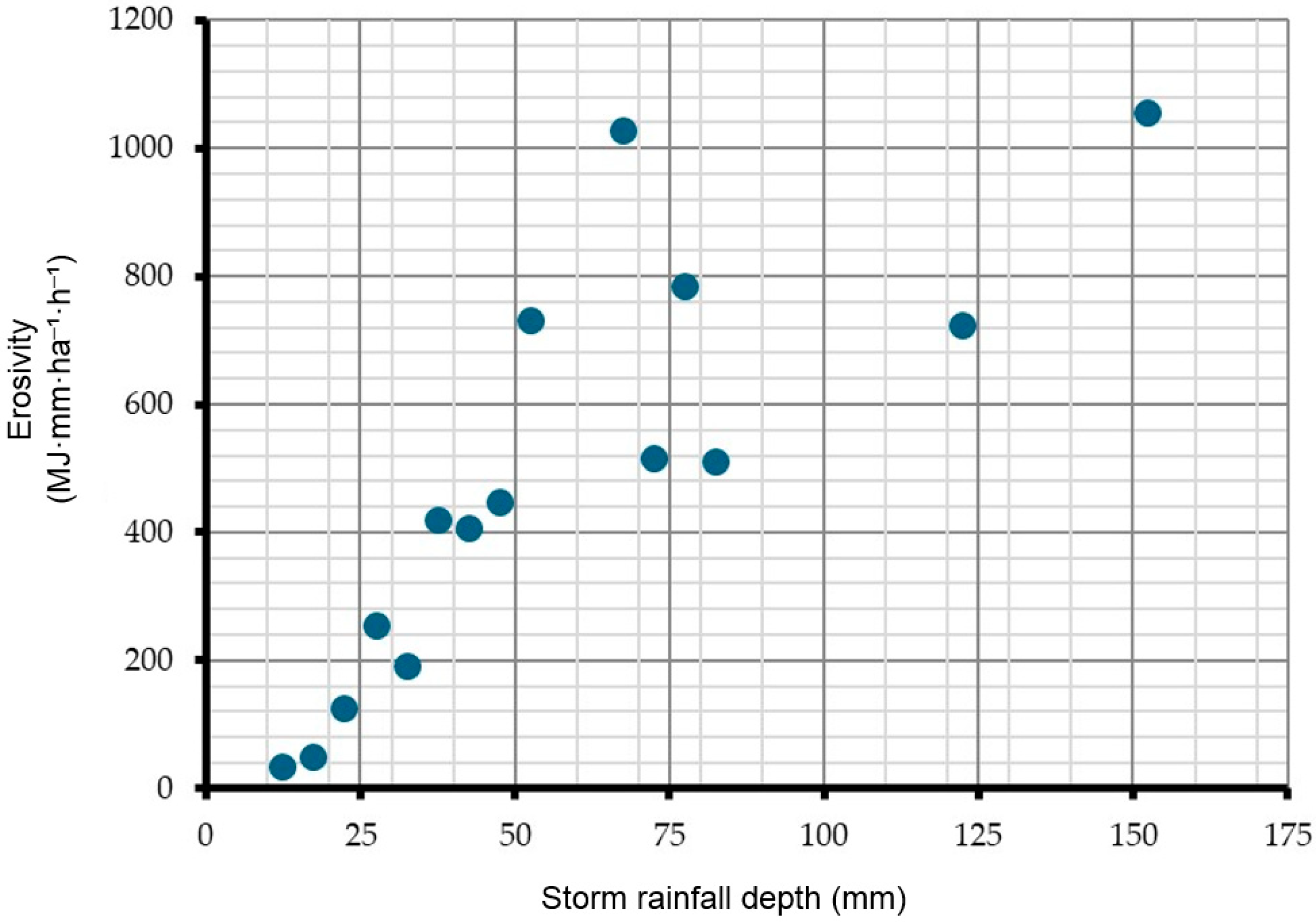
Because the relationship shown in Figure 5 exhibits substantial dispersion, the rainfall series was discretized into 5 mm intervals. Each class interval therefore contains a group of storms with different durations and erosive energies. This discretization facilitates the construction of density histograms for those intervals containing at least 10 observations; the basic elements of this procedure are summarized in

Table 2. Summary statistics used to determine the characteristic erosive energy for each rainfall class interval.

(1)	(2)	(3)	(4)	(5)	(6)	(7)
Lower Limit	Upper Limit	Class Midpoint	Absolute Frequency	Minimum EI30 Value	Maximum EI30 Value	Number of Bins
10	15	12.5	20	5.9	89.8	5
15	20	17.5	10	0.8	110.1	3
20	25	22.5	12	32.3	223.7	3
25	30	27.5	5	89.4	388.8	0
30	35	32.5	7	4.6	444.4	0
35	40	37.5	8	123.8	657.1	0
40	45	42.5	3	226.1	650.9	0
45	50	47.5	3	160.3	733.7	0
50	55	52.5	2	454.6	1004.7	0
65	70	67.5	1	1026.5	1026.5	0
70	75	72.5	2	410.2	619.6	0
75	80	77.5	1	783.5	783.5	0
80	85	82.5	2	502.1	517.1	0
120	125	122.5	2	197.8	1247.1	0
150	155	152.5	1	1054.6	1054.6	0

.

In the example shown in Table 2, density functions were fitted only to the first three class intervals. The histogram for the first interval consists of five bins defined according to the methodology of Freedman and Diaconis [40]. Unlike a frequency histogram, a density histogram is normalized so that the total area of all bins equals one. The histogram is constructed directly from the sample data, and its shape depends strongly on the choice of bin width.

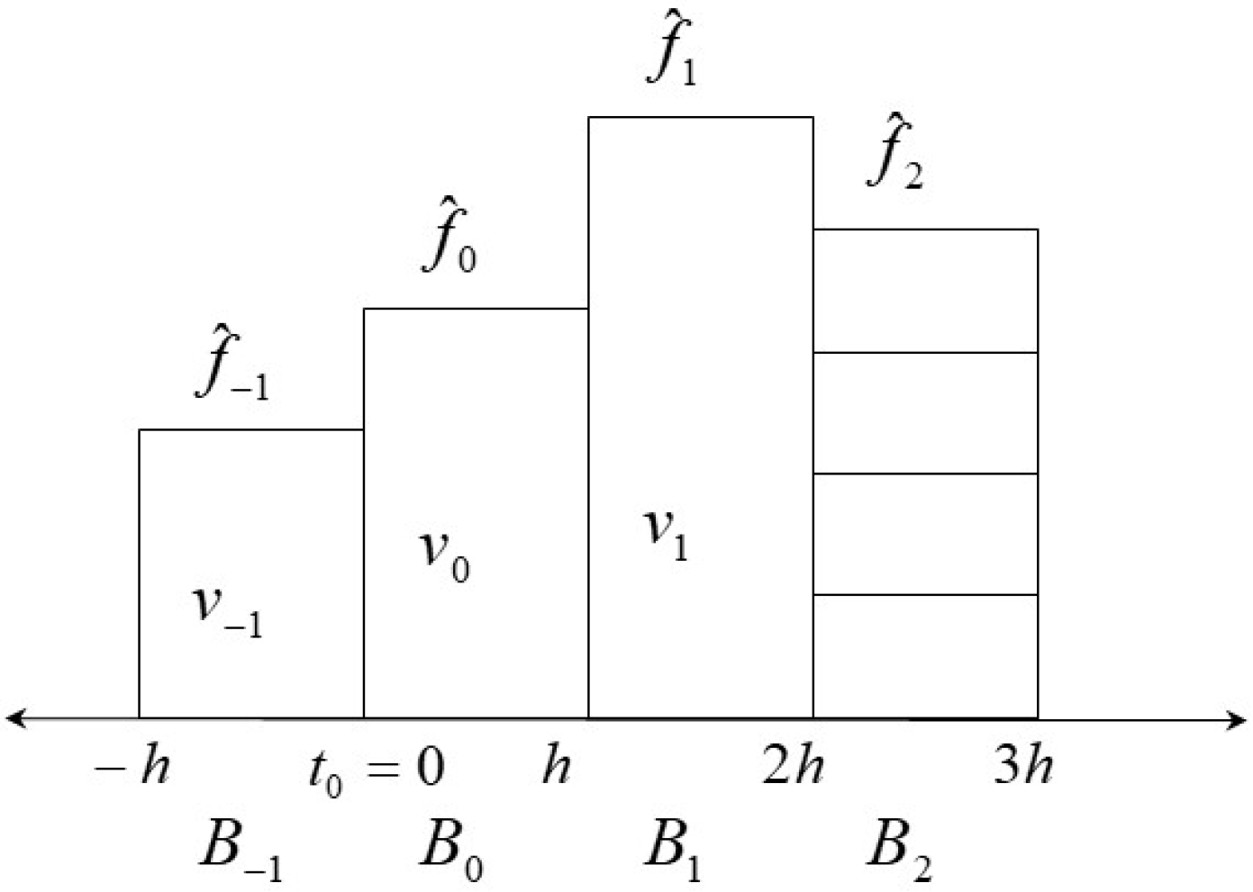
For a histogram with equal-width bins (Figure 6), the density estimator for observations falling in bin $B_k=\left[t_k,t_{k\{1}\right.)$ can be expressed as:

$$\widehat{f}\left(x\right)={\displaystyle \frac{u_k}{nh}}={\displaystyle \frac{1}{nh}}{\sum }_{i=1}^n{I}_{t_k,t_{k\{1}}\left(x_i\right), x\in B_k=\left[t_k,t_{k\{1}\right.)$$

(8)

where h denotes the bin width, $u_k$ is the number of observations in bin k, n is the sample size, and $I_{t_k,t_{k\{1}}\left(·\right)$ is the indicator function of the interval $\left[t_k,t_{k\{1}\right.)$.

The main difficulty in histogram construction lies in selecting an appropriate bin width. Several methods are available for this purpose. Some assume an underlying probability distribution, whereas others optimize the bin width by minimizing an error criterion or producing a stable representation of the data. In this study, the selected bin width was the one that yielded the most consistent histogram with the fewest empty classes.

The methods considered were:

Scott [41]:

$$\widehat{h}=3.5\widehat{\sigma }{n}^{-{\displaystyle \raisebox{1ex}{$1$}\!\left/ \!\raisebox{-1ex}{$3$}\right.}}$$

(9)

Freedman and Diaconis [40]:

$$\widehat{h}=2\left(IQ\right)n^{-{\displaystyle \raisebox{1ex}{$1$}\!\left/ \!\raisebox{-1ex}{$3$}\right.}}$$

(10)

Biased cross-validation [42,43]:

$$BCV(h)={\displaystyle \frac{5}{6nh}}+{\displaystyle \frac{1}{12n^{2}h}}{\sum }_k{\left(v_{k+1}-v_k\right)}^2$$

(11)

Unbiased cross-validation [43]:

$$UCV(h)={\displaystyle \frac{2}{\left(n-1\right)h}}-{\displaystyle \frac{n+1}{n^2\left(n-1\right)h}}{\sum }_k{v_k}^2$$

(12)

Histogram bandwidth optimization [44]:

$$C\left(h\right)={\displaystyle \frac{2k-v}{h^2}}; k={\displaystyle \frac{1}{N}}{\sum }_{i=1}^N{k}_i; v={\displaystyle \frac{1}{N}}{\sum }_{i=1}^N{\left(k_i-k\right)}^2$$

(13)

• Step 3

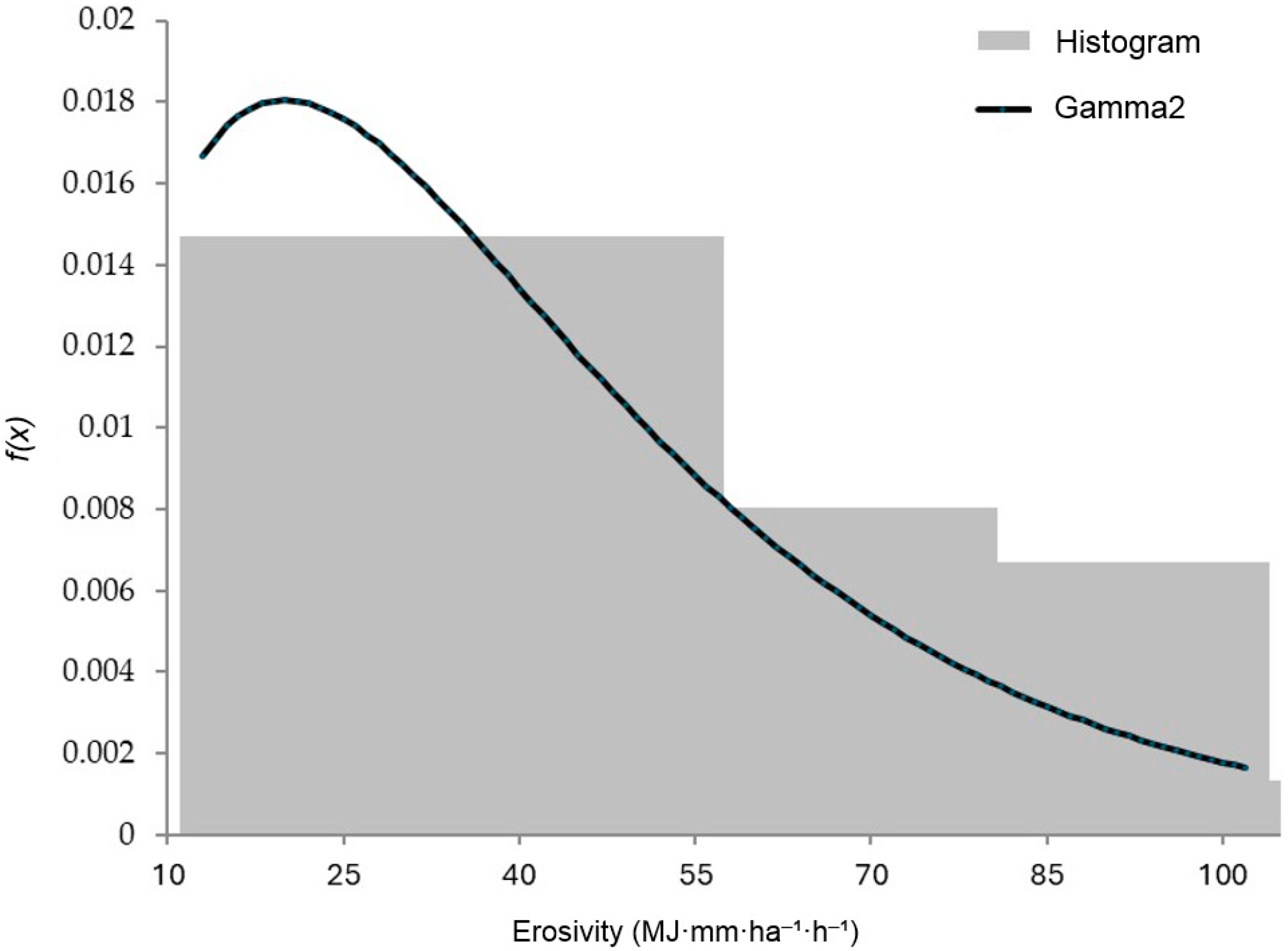
Once the rainfall classes had been defined, each histogram containing at least 10 observations was fitted to the Normal, two-parameter Lognormal, two-parameter Gamma, and Gumbel probability density functions [45]. Figure 7 presents an example of the best-fitting distribution obtained for one class interval. The selected distribution was the one yielding the minimum Standard Error of Fit (SEF), defined as:

$$SEF={\left[{\sum }_{i=1}^n{\displaystyle \frac{{\left({\widehat{X}}_i^j-X_i^j\right)}^2}{n-mp}}\right]}^{{\displaystyle \raisebox{1ex}{$1$}\!\left/ \!\raisebox{-1ex}{$2$}\right.}}$$

(14)

where n is the sample size at site j, ${\widehat{X}}_i$ are the fitted values estimated by the probability distribution under consideration, $x_i$ are the observed values ranked from largest to smallest and associated with their corresponding return periods, and mp is the number of parameters in the distribution.

The expected value of the best-fitting distribution was adopted as the characteristic erosive response for each rainfall class interval. For the first interval in the example shown in Table 2, the best fit was obtained with the two-parameter Gamma distribution, whose expected value is:

$$E\left[x\right]=\widehat{\alpha }\widehat{\beta }$$

(15)

where $\widehat{\alpha }$ and $\widehat{\beta }$ are the estimated parameters of the distribution.

Thus, in this example, the resulting characteristic storm erosivity is valid for storms with daily rainfall totals in the 10–15 mm range. For class intervals with fewer than 10 observations, for which probability distributions could not be fitted reliably, the arithmetic mean of the corresponding data cluster was used as the characteristic erosive response.

• Step 4

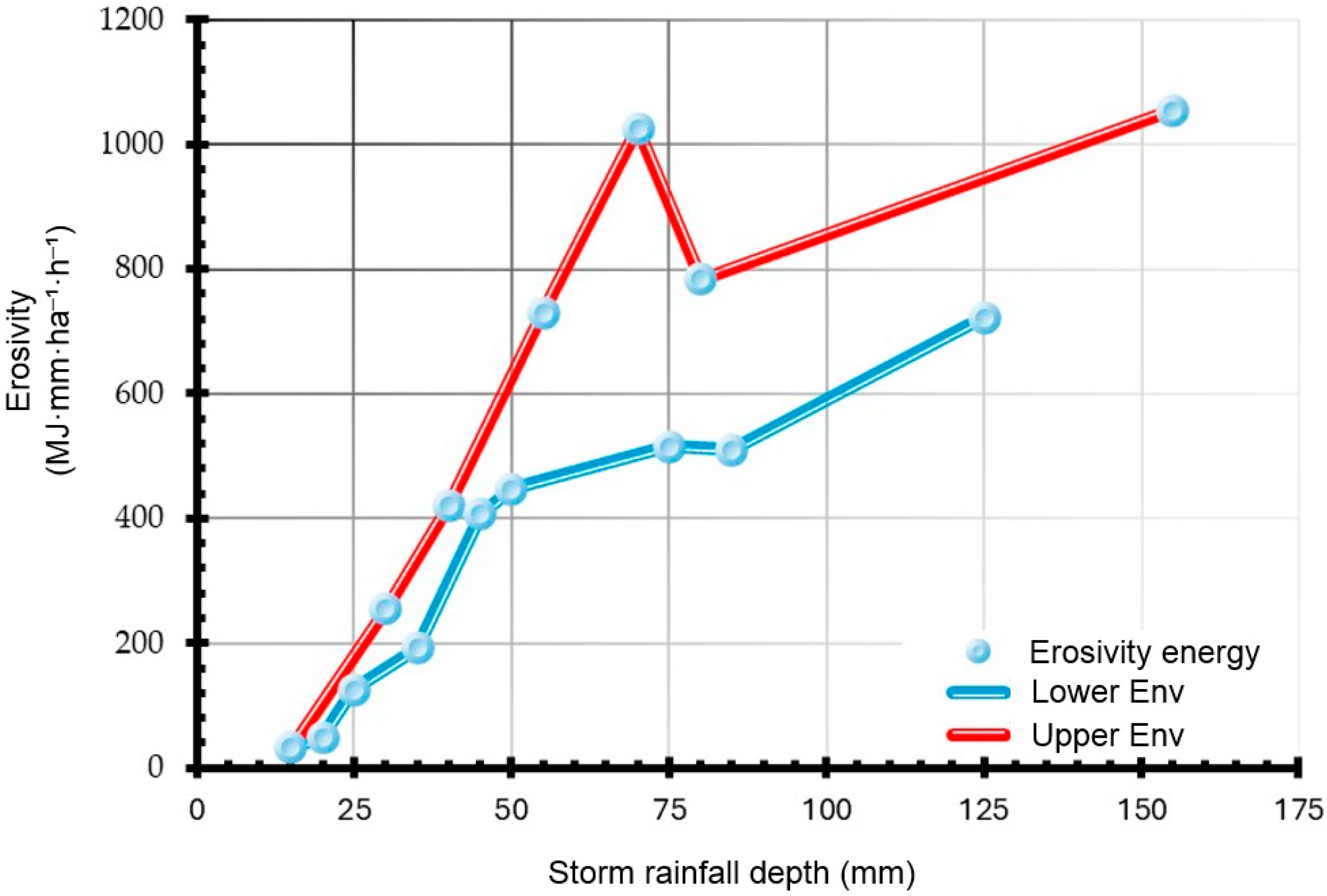
After replacing the raw storm-to-storm variability with characteristic erosive values by rainfall class, dispersion in the original storm rainfall depth–${EI}_{30}$ relationship is substantially reduced. This resulting modified relationship is shown in Figure 8.

In principle, storm erosivity should increase as daily rainfall total increases. However, this relationship is not strictly unique, because storms with similar daily rainfall totals may differ markedly in duration, temporal concentration, and peak intensity. As a result, comparable values of storm rainfall depth produce substantially different values of ${EI}_{30}$. To preserve the physically expected increasing trend while smoothing the residual variability, upper and lower envelopes were traced for the erosivity values associated with the rainfall class marks, as shown in Figure 9.

A nonlinear regression model of the following form was then fitted to these envelopes:

$${EI}_{30}={\displaystyle \frac{a·b+c·x^d}{b+x^d}}$$

(16)

where x represents the daily rainfall total of the storm under evaluation, and a, b, c and d are empirical parameters.

To ensure that Equation (16) was not selected solely on theoretical grounds, its functional form was also evaluated empirically against alternative candidate relationships fitted to the modified rainfall depth-storm erosivity data obtained in Step 4. The tested formulations included linear, power, exponential, logarithmic, and bounded nonlinear models. Each equation was fitted to the rainfall-class data by least squares, and performance was compared using statistical fit criteria together with physical consistency over the observed rainfall range. In addition to goodness of fit, candidate equations were screened according to whether they preserved a monotonic increase in erosivity with rainfall depth and whether they avoided unrealistic oscillations or negative predictions. Under this combined criterion, the four-parameter bounded form of Equation (16) was retained because it provided the most favorable balance between empirical fit and physical consistency for the present application.

Equation (16) can also be written as:

$${EI}_{30}=a+{\displaystyle \frac{\left(c-a\right)x^d}{b+x^d}}$$

which facilitates the interpretation of its parameters. In this form, parameter a represents the lower asymptotic erosivity, that is, the baseline erosivity level approached for low rainfall totals. Parameter c represents the upper asymptotic erosivity, or the maximum characteristic erosivity approached as rainfall total increases. Parameter b controls the horizontal position of the transition between these two asymptotic levels and therefore defines a characteristic rainfall scale for the increase in erosivity. In particular, when $x= b^{1/d}$, the predicted value of ${EI}_{30}$ reaches the midpoint between a and c. Finally, parameter d is a dimensionless shape parameter that controls the curvature and steepness of the relationship; larger values of d produce a sharper transition, whereas smaller values produce a more gradual increase.

From a physical standpoint, these parameters summarize the dominant features of the local rainfall–erosivity regime. Parameter a reflects the lower-limit erosive response associated with relatively small erosive storms, whereas c reflects the characteristic upper-limit response associated with large daily rainfall totals. 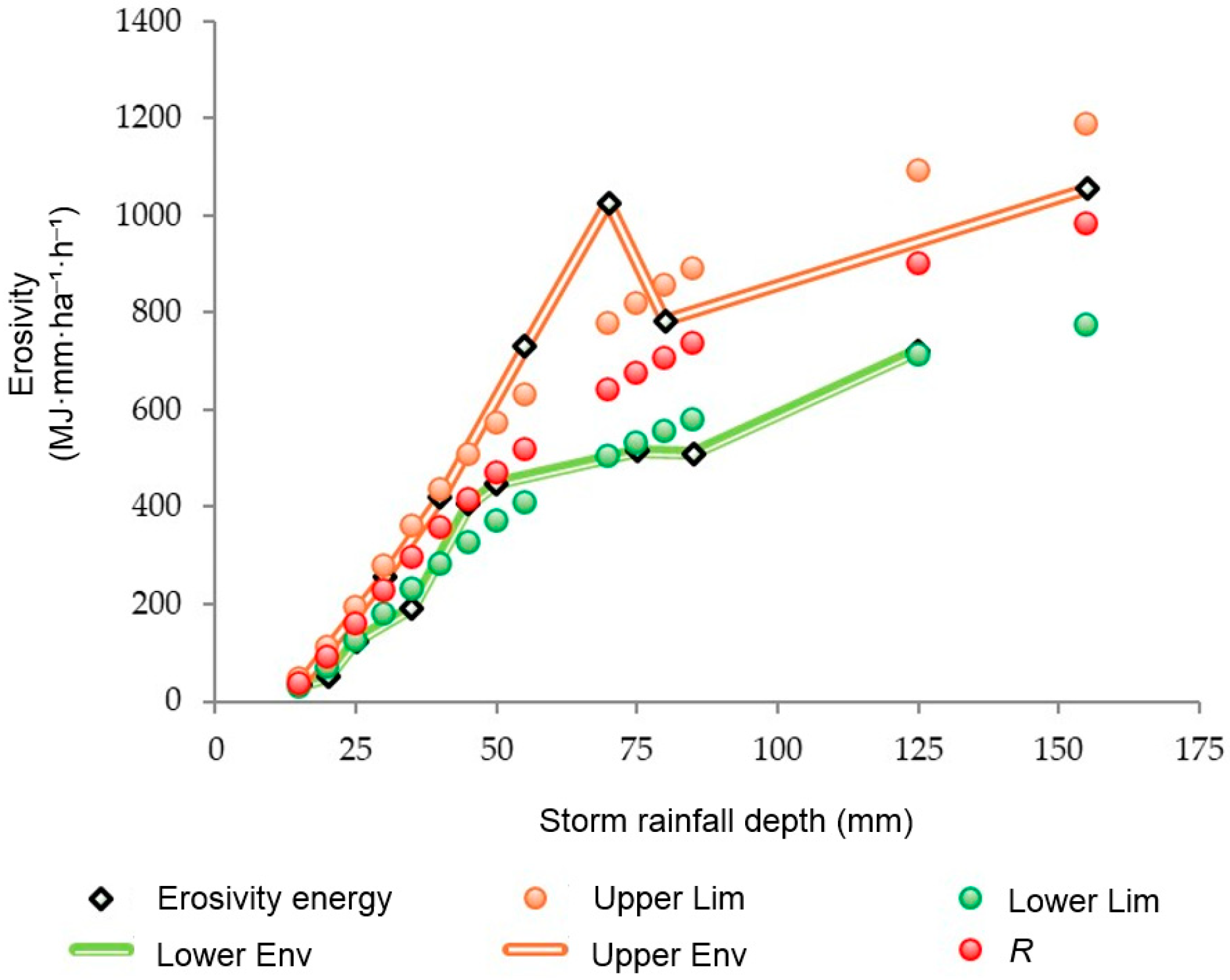Parameter b indicates the rainfall amount at which the increase in erosivity becomes most pronounced, and parameter d reflects the sensitivity of erosivity to changes in daily rainfall around that transition range. The final fitted relationship between daily rainfall total and storm erosivity is shown schematically in Figure 10.

• Step 5

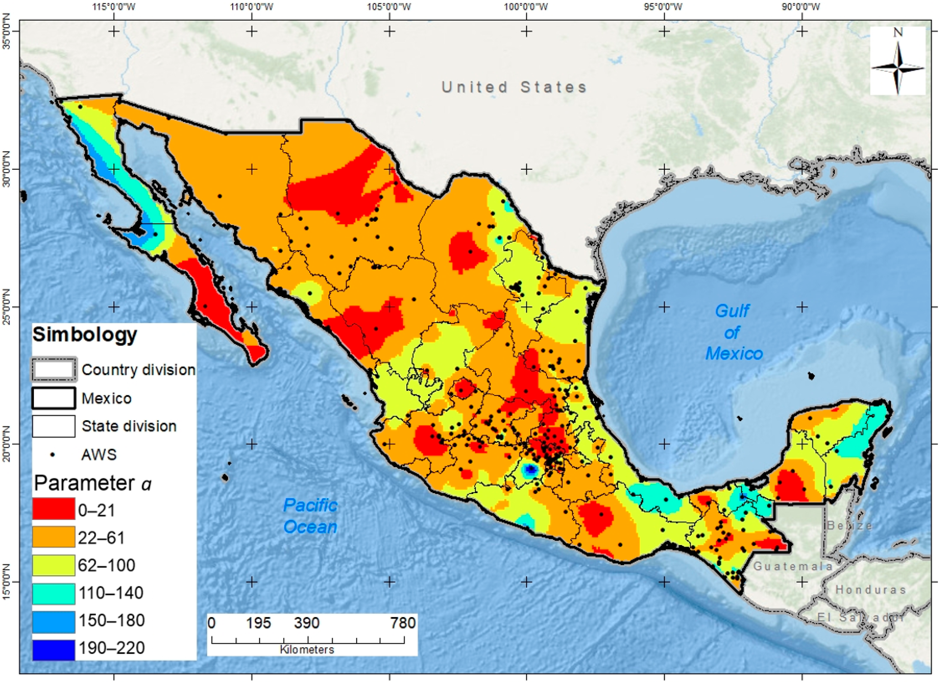
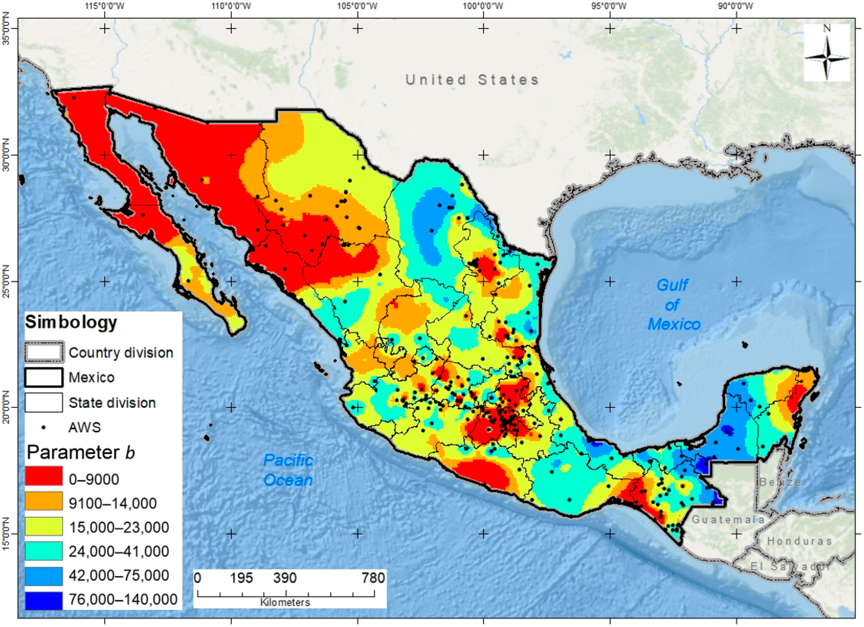
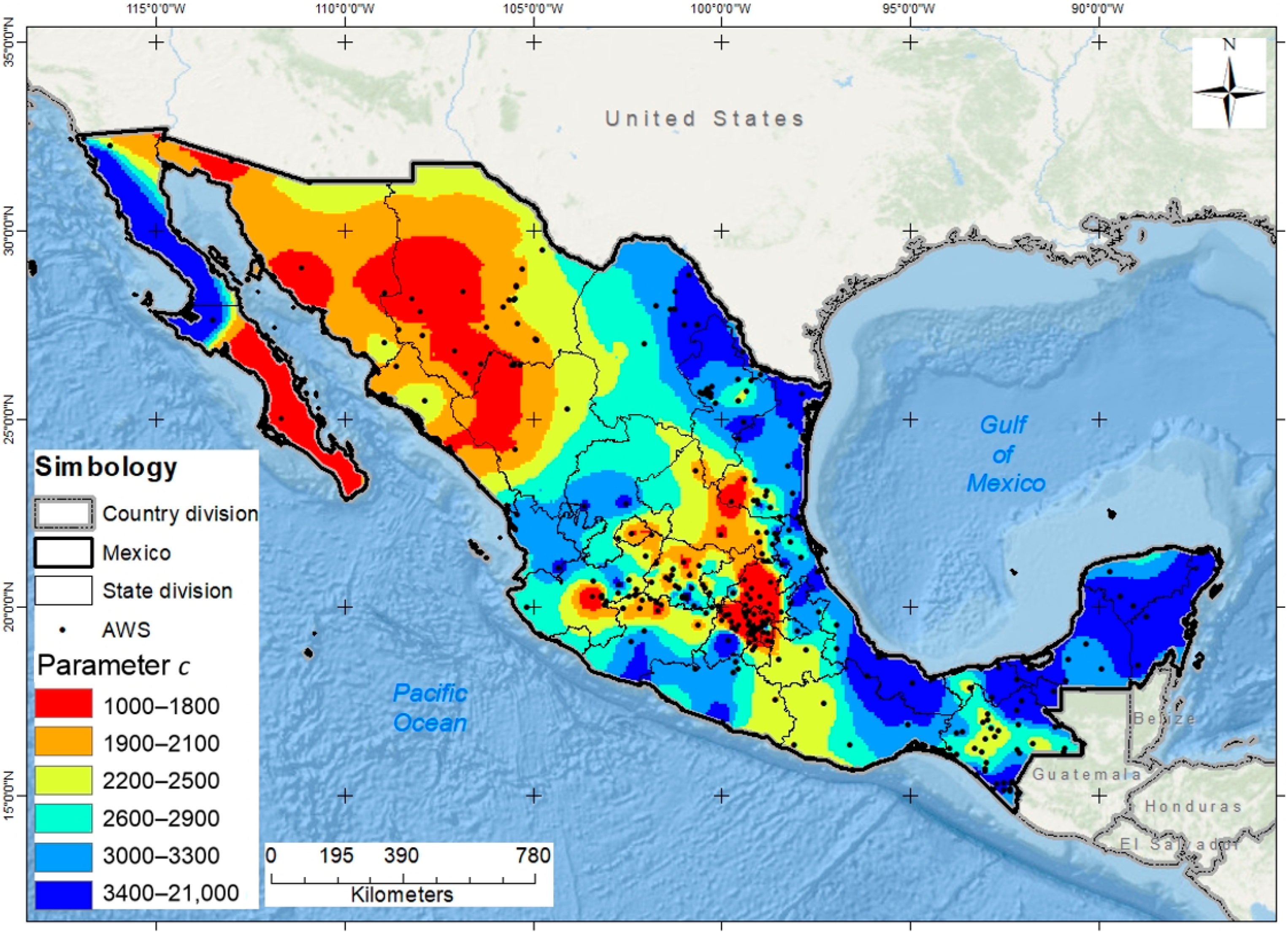
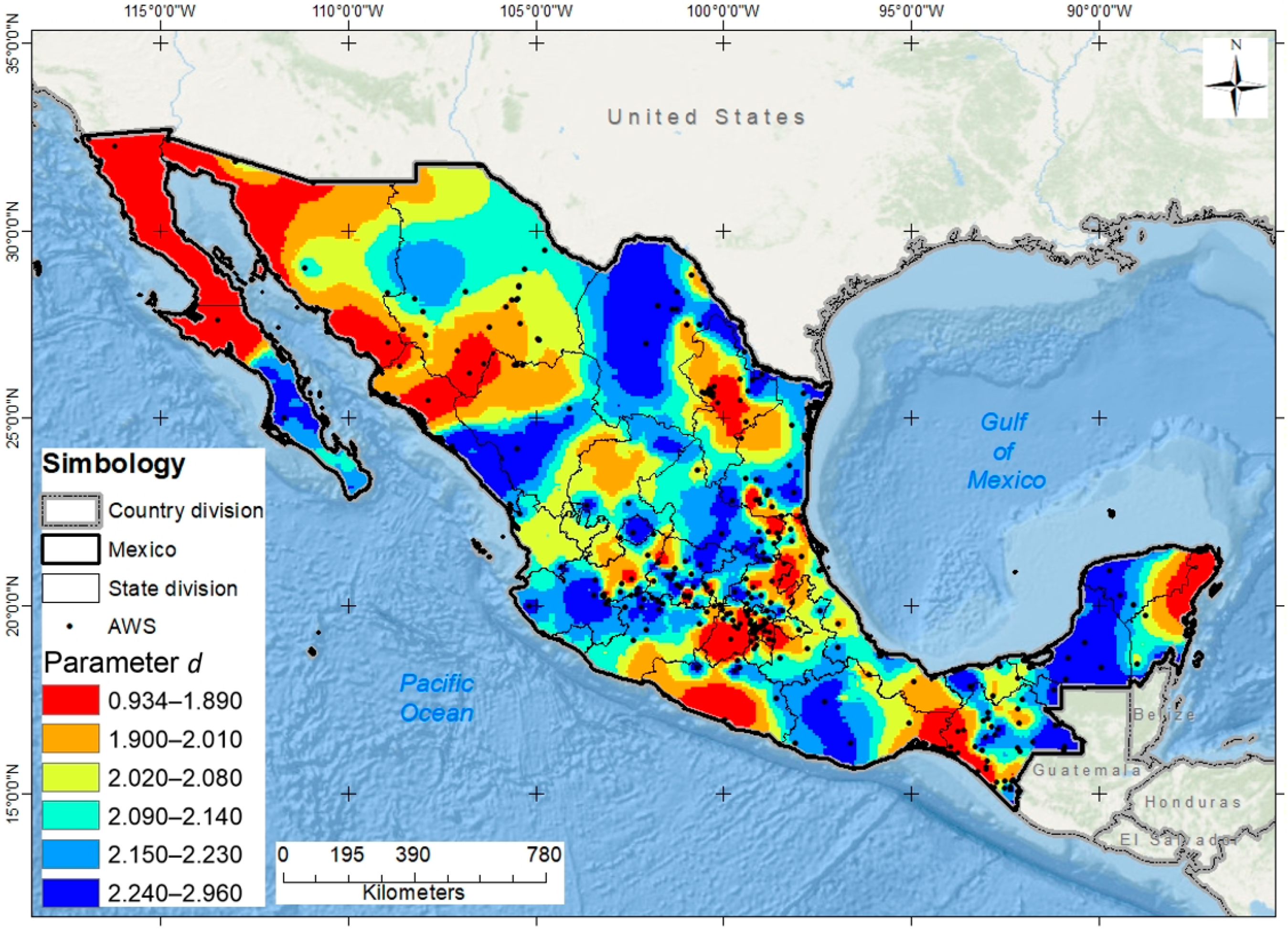
Once the fitting parameters a, b, c and d of Equation (16) were determined for each AWS, continuous parameter fields were generated by inverse distance weighting (IDW) interpolation. These parameter maps make it possible to transfer the calibrated rainfall-erosivity relationship from the automatic weather stations to the broader climatological network. Using these interpolated parameter fields together with daily rainfall totals recorded at a given climatological station, the storm erosivity of each erosive day can be estimated through Equation (16). Annual rainfall erosivity is then reconstructed by summing the estimated event erosivities over all erosive days in each year, according to Equation (7). In this way, the year-to-year variation in the annual rainfall erosivity factor can be reproduced from daily rainfall data, as illustrated schematically in Figure 11.

2.5. Rationale for IDW and Station-Based Validation Framework

IDW was adopted in this study for two purposes: infilling missing daily rainfall values within homogeneous regions and interpolating the fitted parameters of Equation (16) from AWS locations to the broader climatological network. The method was selected because it provides a transparent, computationally efficient, and exact interpolation framework that can be implemented directly from the observed data without requiring prior estimation of spatial covariance structure. This property is particularly advantageous in a national-scale application such as the present one, where the monitoring network is spatially irregular and locally sparse in some regions, which may limit robust semivariogram estimation for kriging-based approaches. In contrast to nearest-neighbor methods, IDW produces a gradual spatial transition, and unlike spline-based methods, it preserves a stronger local dependence on nearby observations. For these reasons, IDW was considered an operationally appropriate choice for consistent large-scale implementation in the present study.

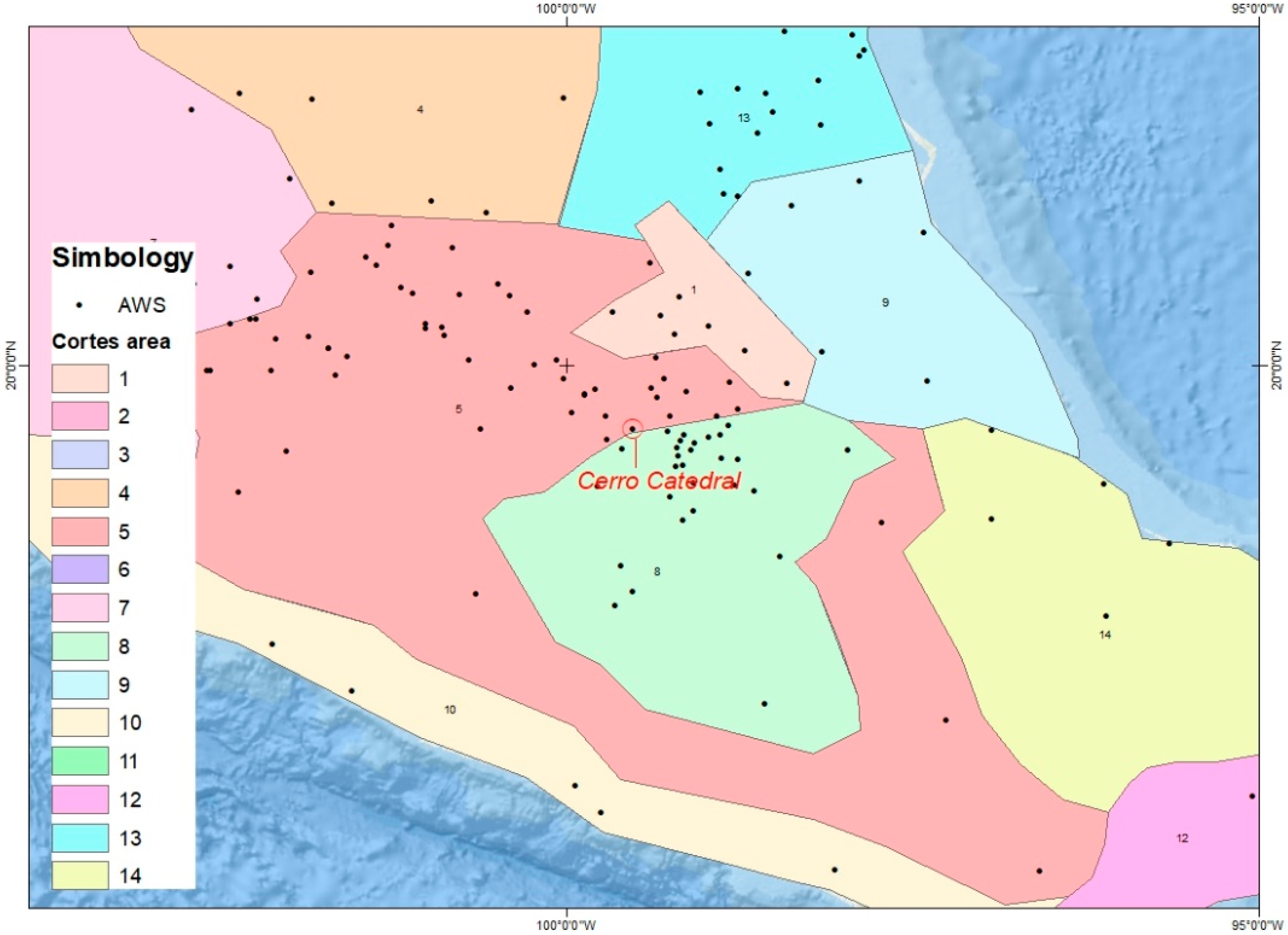
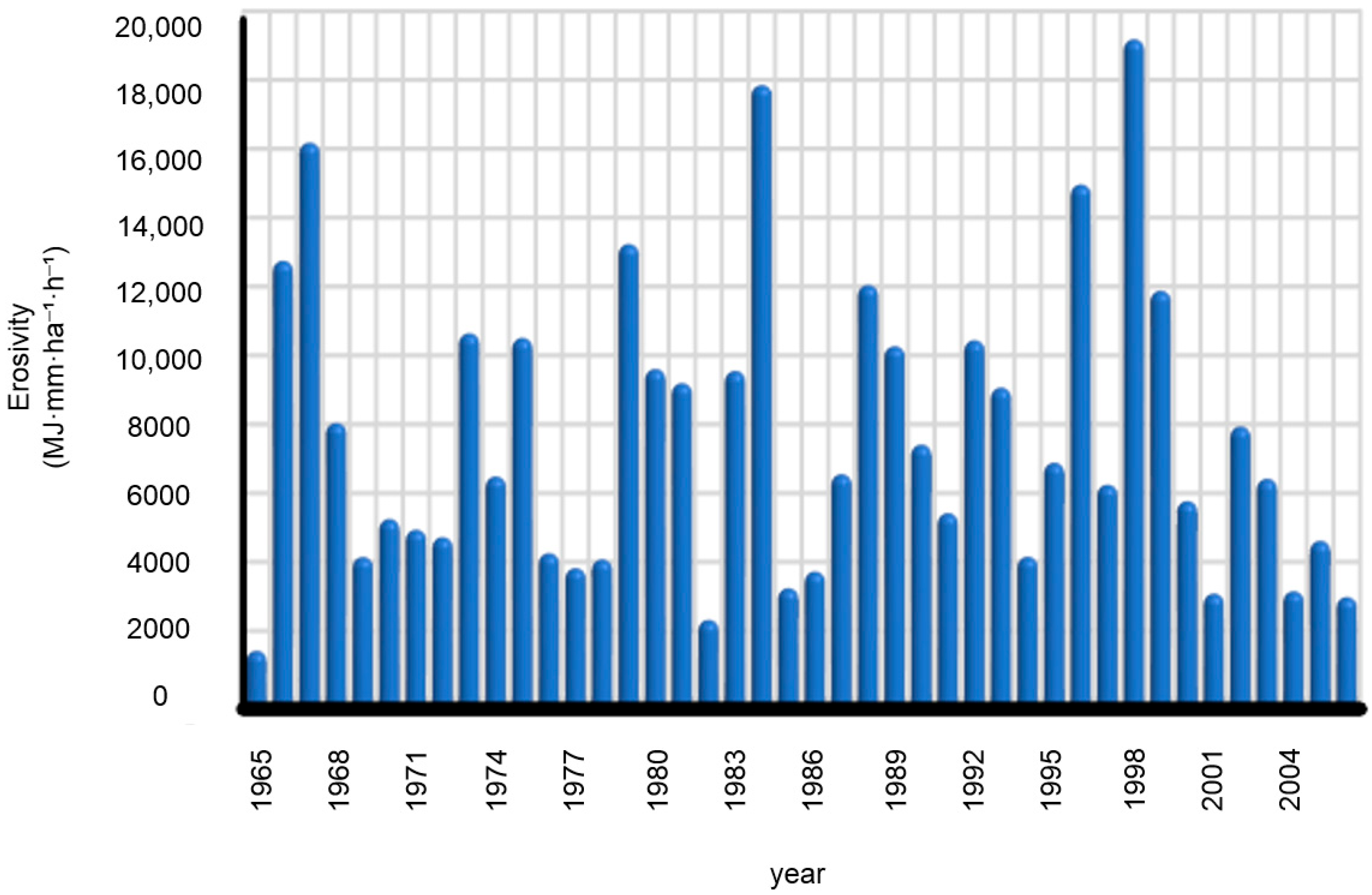
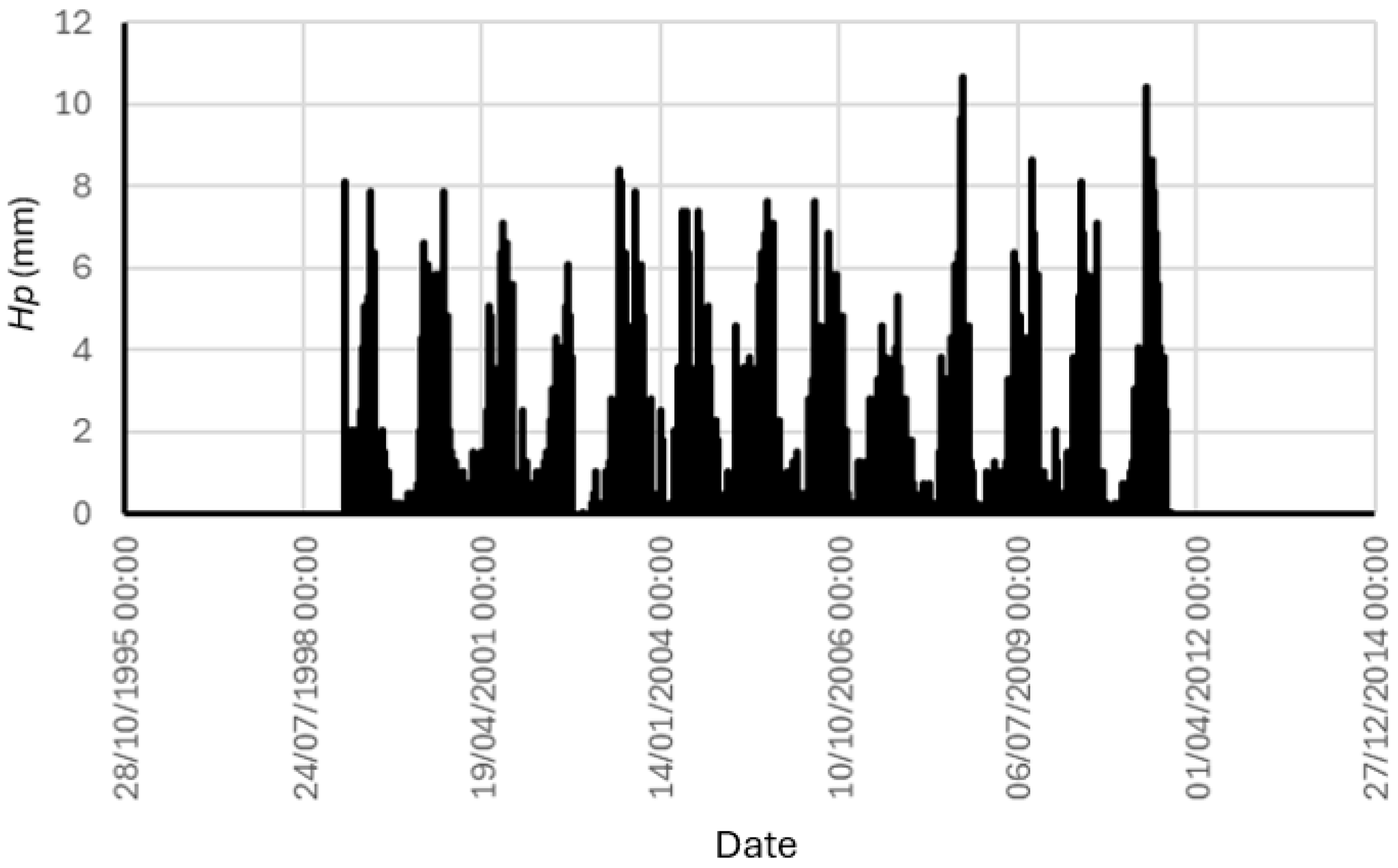
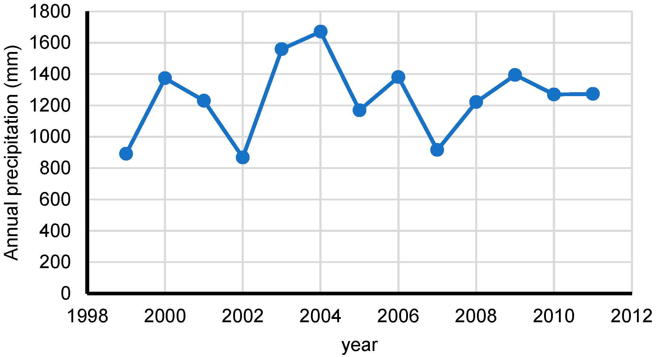
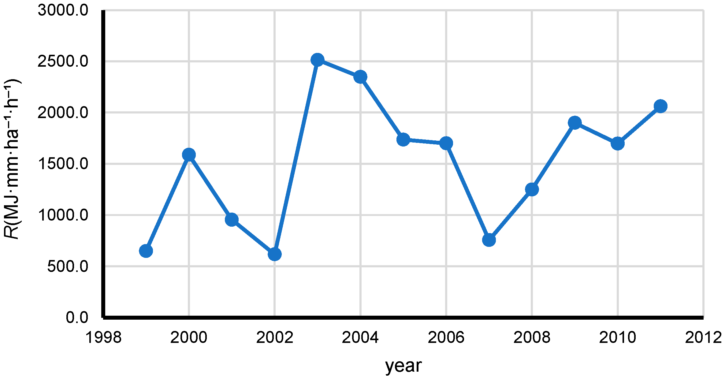
To provide a direct quantitative comparison between the proposed methodology and the regional equations of Cortes [34], a station-based validation was conducted using the Cerro Catedral Automatic Weather Station (AWS) as a case study. This station was selected because it contains continuous precipitation records at 10 min intervals, which made it possible to derive a reference annual erosivity series directly from high-temporal-resolution rainfall observations. The purpose of this comparison was not to evaluate a large set of alternative predictive models, but rather to contrast the proposed daily rainfall-based formulation with the regional approach that remains one of the most widely used methodologies for estimating rainfall erosivity in Mexico.

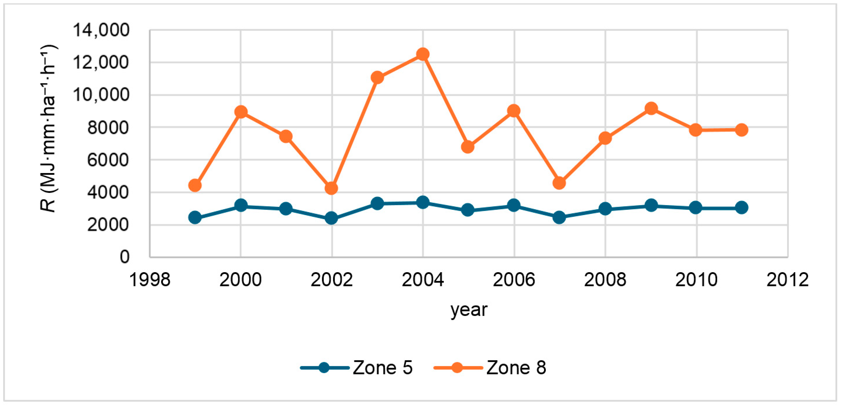
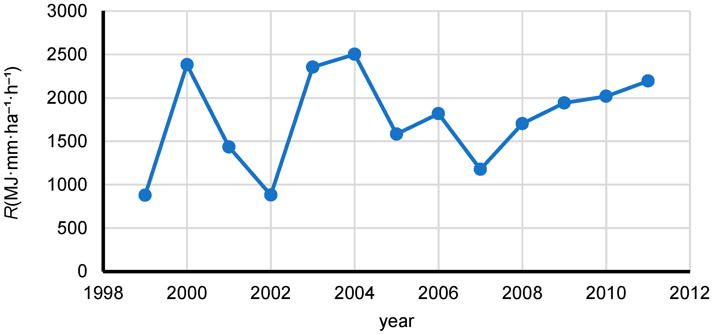
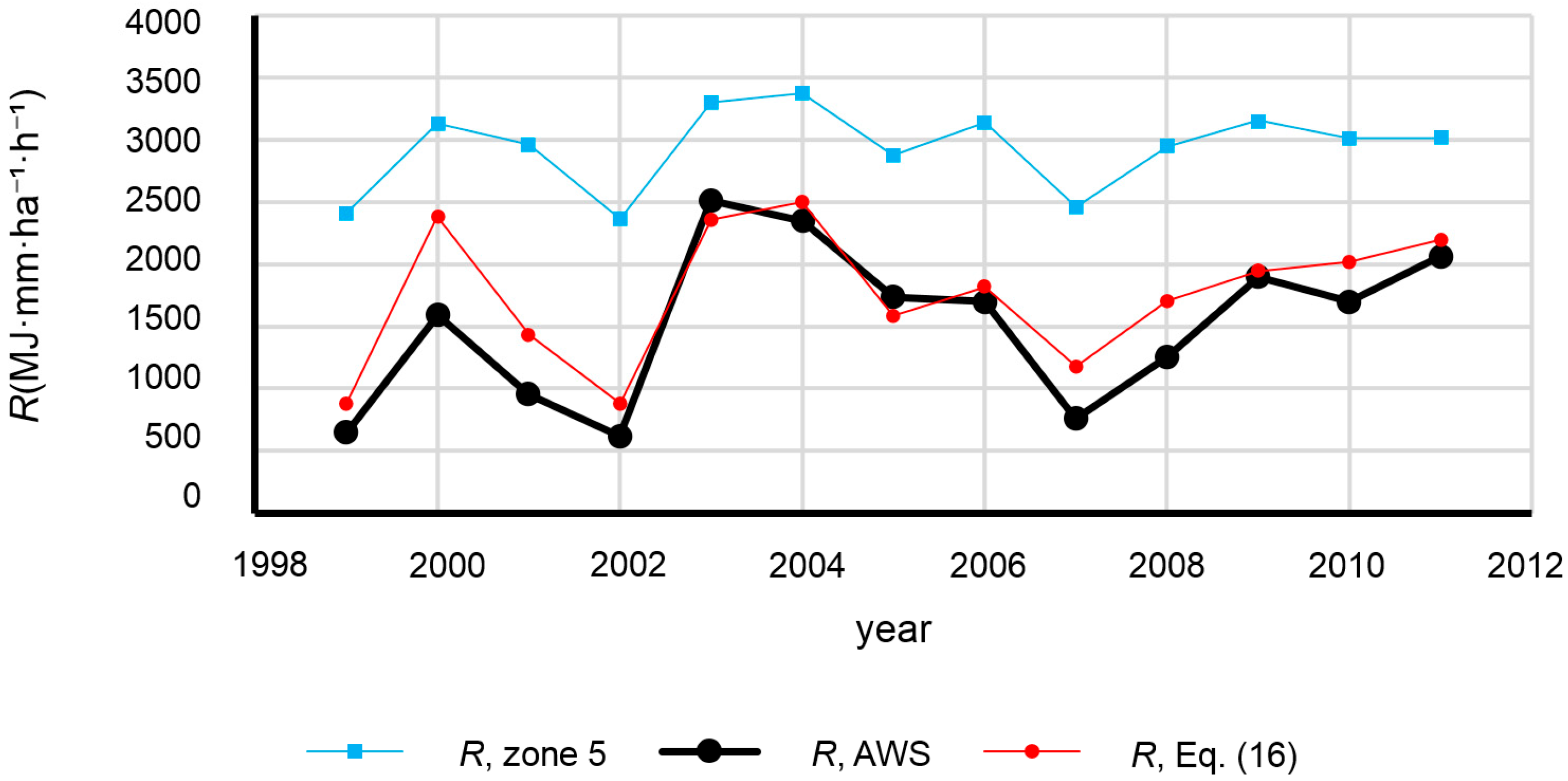
For the Cerro Catedral AWS, annual erosivity was first computed directly from the 10 min rainfall record through Equations (6) and (7), thereby producing the reference annual series. The same station was then evaluated using the regional equations of Cortés, based on annual precipitation, and with Equation (16), based on daily precipitation totals. Comparative performance was quantified with the standard error of fit (SEF), using the storm-derived annual erosivity series as the reference. This formulation was adopted because it allows for comparison between the competing approaches while partially accounting for their different levels of complexity through the parameter term in the denominator. The resulting comparison is presented in Section 3.1.

3. Results

The results are presented in four stages. First, a station-based comparison between the proposed methodology and the regional equations of Cortés [34] is presented using the Cerro Catedral AWS as a validation case. Second, the spatial behavior of the parameters of Equation (16) is described. Third, these parameters are combined with the daily rainfall records from the climatological network to estimate the national-scale distribution of the annual rainfall erosivity factor. Fourth, a basin-scale comparison is presented for the Paso de la Reyna watershed.

3.1. Station-Based Comparison Between Equation (16) and the Cortes Methodology

To provide a direct quantitative comparison between the methodology proposed in this study and the regional equations of Cortés [34], a station-based validation was conducted using the Cerro Catedral Automatic Weather Station (AWS) as a case study. This station was selected because it contains continuous precipitation records at 10 min intervals from 13 March 1999 to 31 December 2011, which made it possible to derive a reference annual erosivity series directly from high-temporal-resolution rainfall observations. The purpose of this comparison was not to evaluate a large set of alternative predictive models, but rather to contrast the proposed daily rainfall-based formulation with the regional approach that remains one of the most widely used methodologies for estimating rainfall erosivity in Mexico.

Figure 12 shows the precipitation record at 10 min resolution for the Cerro Catedral AWS, and Figure 13 presents the corresponding annual precipitation totals. During the analysis period, 2112 rainfall events were identified, of which 315 were classified as erosive according to the criterion adopted in this local comparison. For each erosive storm, the storm erosivity index was computed from the 10 min precipitation record using Equation (6), and the annual rainfall erosivity factor was then obtained using Equation (7). The resulting annual reference series derived directly from the 10 min data is shown in Figure 14.

The geographic coordinates of the Cerro Catedral AWS (19.541944, −99.519167) place the station within Zone V of the erosivity regionalization proposed by Cortés [34], although the site is located approximately 3 km from the boundary with Zone VIII. Because of this proximity, both regional equations were evaluated to examine the sensitivity of the estimated annual erosivity to the assigned zone. The equations are:

R = 3.4880P − 0.00088P² for Zone V

R = 1.9967P + 0.003270P² for Zone VIII

where P is annual precipitation. Figure 15 shows the location of the Cerro Catedral AWS relative to the erosivity zones defined by Cortes. Using the annual precipitation totals shown in Figure 13, annual erosivity was estimated with both regional equations, and the resulting series are presented in Figure 16. The difference between the two zone-based estimates was considerable; on average, the values obtained with the Zone VIII equation were approximately 2.5 times greater than those obtained with the Zone V equation. This result illustrates the sensitivity of the Cortés methodology to regional-zone assignment, especially for stations located near zone boundaries.

For the same station, annual erosivity was also estimated using the nonlinear model proposed in this study, Equation (16), applied to the daily precipitation record. The fitted parameters obtained for the Cerro Catedral AWS were:

a = 0, b = 9744.9627, c = 2450.8891, d = 1.6862

Application of Equation (16) to the daily rainfall series yielded the annual erosivity estimates shown in Figure 17. Figure 18 compares the annual R series obtained from the storm-based reference data, the Cortes equations, and the proposed methodology.

To quantify comparative performance, the standard error of fit (Equation (14)). This formulation was adopted because it allows for comparison between the competing approaches while partially accounting for their different levels of complexity through the term mp. For the Cortés methodology, taking mp = 2 and a record length of 13 years, the SEF was 1455.77 MJ·mm·ha⁻¹·h⁻¹·yr⁻¹. For the proposed methodology based on Equation (16), taking mp = 4 and the same record length, the SEF was 347.00 MJ·mm·ha⁻¹·h⁻¹·yr⁻¹.

For the Cerro Catedral case study, Equation (16) reproduced the reference annual erosivity series more closely than the Cortes regional equations. Even after accounting for the larger number of fitted parameters through the SEF expression, the proposed methodology showed a substantially smaller fitting error. This result indicates that, at least for this station, the daily rainfall-based nonlinear model captures the annual variability of rainfall erosivity more consistently than the regional annual-precipitation equations. This comparison should be interpreted as a focused validation against the principal benchmark methodology used in Mexico, rather than as a universal demonstration of superiority over all possible alternative models or under all hydroclimatic conditions.

3.2. Spatial Behavior of the Parameters of Equation (16)

Application of the proposed methodology to the 170,796 storms recorded at the 432 Automatic Weather Stations yielded representative values of the parameters a, b, c and d in Equation (16). Their spatial distributions, obtained by inverse-distance weighting (IDW) interpolation, are shown in Figure 19, Figure 20, Figure 21 and Figure 22.

The interpolated parameter fields show that the rainfall-erosivity relationship is not spatially uniform across Mexico. Instead, the fitted coefficients vary in a manner that reflects the marked hydroclimatic contrasts of the country. This result supports the use of a spatially distributed transfer framework rather than a single nationwide equation.

3.3. National Scale Distribution of Annual Rainfall Erosivity

Once these parameter fields were obtained, they were combined with the daily rainfall totals greater than 10 mm recorded at the 2124 climatological stations during the common period 1965–2006. This integration made it possible to estimate the spatial distribution of annual rainfall erosivity across Mexico through Equations (7) and (16). The resulting national pattern is shown in Figure 23.

At the national scale, the estimated erosivity field shows a marked contrast between the arid and semi-arid north and northwest of Mexico, where annual erosivity is generally low, and the humid and subhumid regions of central, southern, and southeastern Mexico, where erosivity increases substantially. The lowest values are concentrated in Baja California, northwestern Mexico, and broad sectors of the northern plateau, whereas the highest values are observed mainly in the south and southeast, with particularly elevated erosivity in portions of the Gulf-facing and southern Pacific regions.

3.4. Basin-Scale Comparison in the Paso de la Reyna Watershed

To further examine the practical implications of the proposed methodology, its results were compared with those obtained using the regional equations of Cortes [34] in the Paso de la Reyna watershed. For this basin-scale case study, hydrometric station 20017, known as “Paso de la Reyna,” was used as the reference location. This station is located at 16°16′30″ N and 97°36′30″ W, in the municipality of Jamiltepec, Oaxaca. Figure 24 shows the watershed delineated for this station, the location of the climatological stations used in the analysis, and the corresponding areas of influence assigned through Thiessen polygons. The rainfall record analyzed covers the period 1965–2006.

As a reference for the subsequent comparison, Figure 25 presents the spatial distribution of mean annual rainfall within the basin for the period 1965–2006. The rainfall field exhibits clear internal spatial contrasts that provide a useful benchmark for interpreting the corresponding erosivity estimates.

Using the proposed methodology, Figure 26 shows the spatial distribution of the mean annual rainfall erosivity factor estimated from daily rainfall totals greater than 10 mm over the same period. The resulting field is spatially differentiated and broadly consistent with the rainfall gradients shown in Figure 25.

For comparison, Figure 27 presents the spatial distribution of the mean annual rainfall erosivity factor estimated from annual precipitation using the method proposed by Cortés [34]. Relative to the rainfall pattern shown in Figure 18, this approach exhibits lower spatial consistency and, in some areas, appears to underestimate erosivity. Such differences may affect subsequent estimates of soil loss and sediment yield within the watershed.

4. Discussion

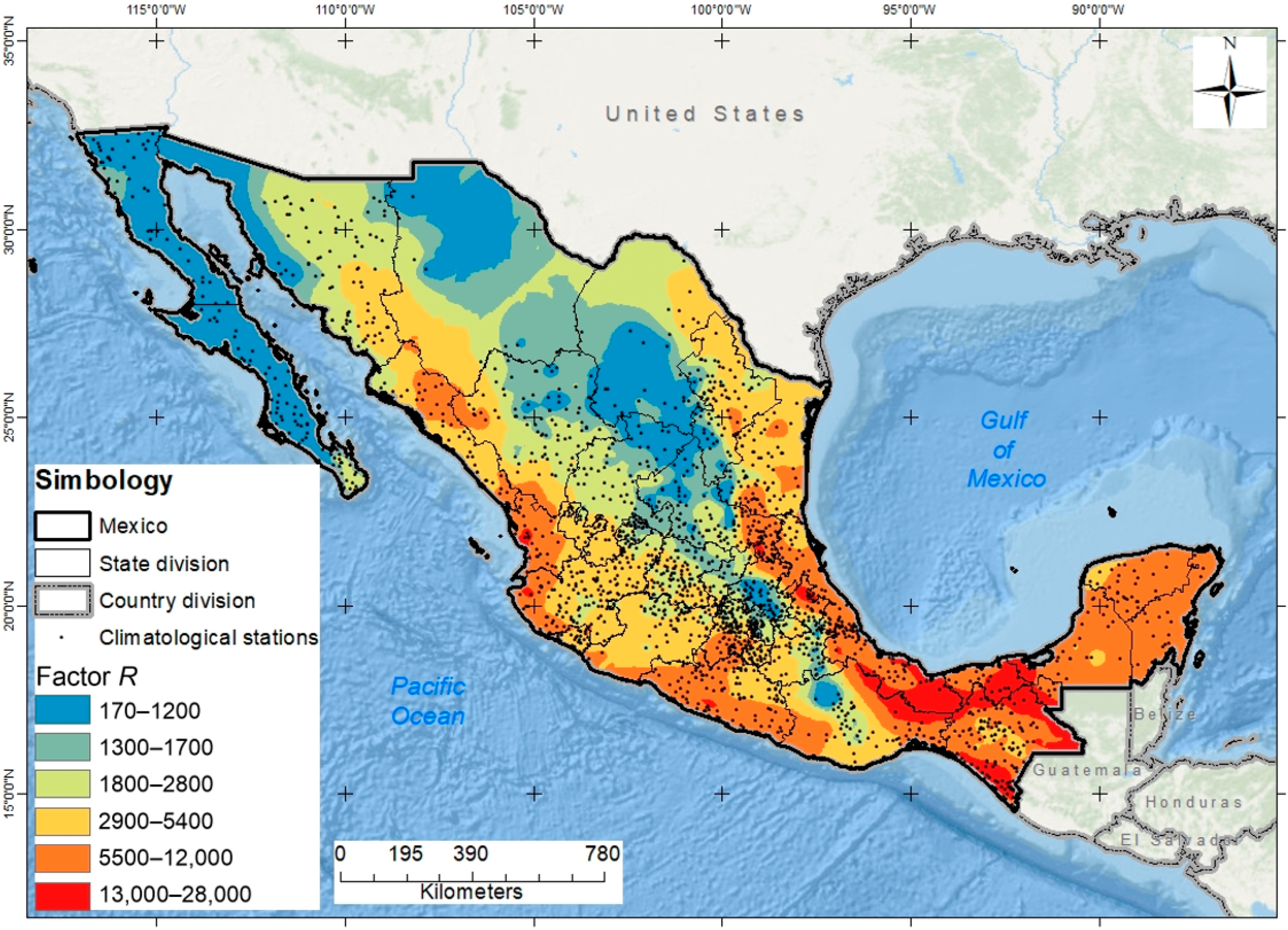
The national pattern shown in Figure 23 reveals a marked contrast between the arid and semi-arid north and northwest of Mexico, where annual rainfall erosivity is generally low, and the humid and subhumid regions of central, southern, and southeastern Mexico, where erosivity increases substantially. This large-scale pattern is physically consistent with the principal gradients of precipitation amount, storm intensity, and seasonal rainfall concentration across the country, and therefore suggests that the proposed methodology reproduces the dominant hydroclimatic controls on erosive forcing with reasonable spatial realism.

Figure 23 also indicates that the national distribution of rainfall erosivity is not spatially uniform within broad climatic regions, but instead exhibits pronounced local and regional contrasts. In several parts of the country, relatively sharp transitions occur over short distances, which likely reflect the combined influence of topography, moisture availability, storm organization, and convective rainfall intensity. This feature is important because it shows that rainfall erosivity in Mexico cannot be adequately represented by overly broad regional equations based only on annual precipitation totals. Rather, the results support the premise that a daily rainfall-based methodology calibrated using sub-daily storm information can provide a spatially detailed representation of erosive forcing that is consistent with the main hydroclimatic contrasts of the country.

This interpretation is consistent with recent international literature. Recent studies continue to show that rainfall erosivity remains an active field of methodological development, particularly in regions where sub-daily intensity data are limited and daily rainfall records are more widely available [2,9]. Dela Cruz et al. [2], for example, proposed an empirical erosivity equation for a tropical data-scarce setting, emphasizing the need for practical estimation frameworks when direct computation of EI₃₀ is not feasible. Oliveira-Roza et al. [31] highlighted the importance of spatially extensive erosivity datasets at the national scale in Brazil, while Fofang et al. [3] showed that rainfall erosivity can respond measurably to long-term changes in rainfall and land-cover conditions in Ethiopia. Likewise, Miao et al. [32] reported that the suitability of erosivity-related factors may vary with watershed conditions and modeling objectives. Taken together, these studies support the broader relevance of the present results: in hydroclimatically heterogeneous countries, erosivity assessment may benefit from methods that explicitly preserve spatial gradients rather than relying only on coarse regional regressions.

From an applied standpoint, the national pattern shown in Figure 23 has important implications for land and water management. Regions with high annual erosivity are likely to be more susceptible to rainfall-driven soil detachment and sediment production, particularly where steep slopes, erodible soils, sparse vegetation cover, or intensive land use are also present. Conversely, the lower values observed in northern Mexico suggest lower mean erosive forcing, although intense local storms may still generate substantial soil loss where surface conditions are vulnerable. In practical terms, the map in Figure 23 provides more than a descriptive national overview: it offers a spatial basis for prioritizing watershed protection, erosion monitoring, sediment-control measures, land-restoration actions, and conservation planning in areas subject to greater erosive pressure. In this sense, the proposed methodology may improve the physical basis of subsequent RUSLE applications aimed at soil-loss estimation, sediment-yield studies, and territorial planning.

More broadly, the pattern in Figure 23 reinforces the importance of representing rainfall erosivity with sufficient spatial detail in countries such as Mexico, where climatic and physiographic heterogeneity is pronounced. National erosion assessments based on sparse pluviographic records or coarse regional regressions may smooth out critical gradients in erosive potential and therefore underestimate local variability in erosion risk. By contrast, the present methodology preserves these gradients more effectively by linking storm-scale erosivity information derived from AWS records with the denser climatological network through a daily rainfall-based transfer relationship. This feature is particularly relevant in Mexico, where daily rainfall records are much more spatially extensive than long sub-daily series.

The station-based comparison at Cerro Catedral provides a direct quantitative point of reference for interpreting these broader patterns. For that case study, Equation (16) reproduced the annual erosivity series derived from 10 min rainfall records much more closely than the regional equations of Cortes, even when the larger number of fitted parameters in Equation (16) was considered through the SEF formulation. This result does not establish universal superiority under all conditions, but it does indicate that, where daily rainfall information is available and a locally calibrated transfer relationship can be applied, the proposed framework can capture interannual erosivity variability more consistently than a regional formulation based only on annual precipitation.

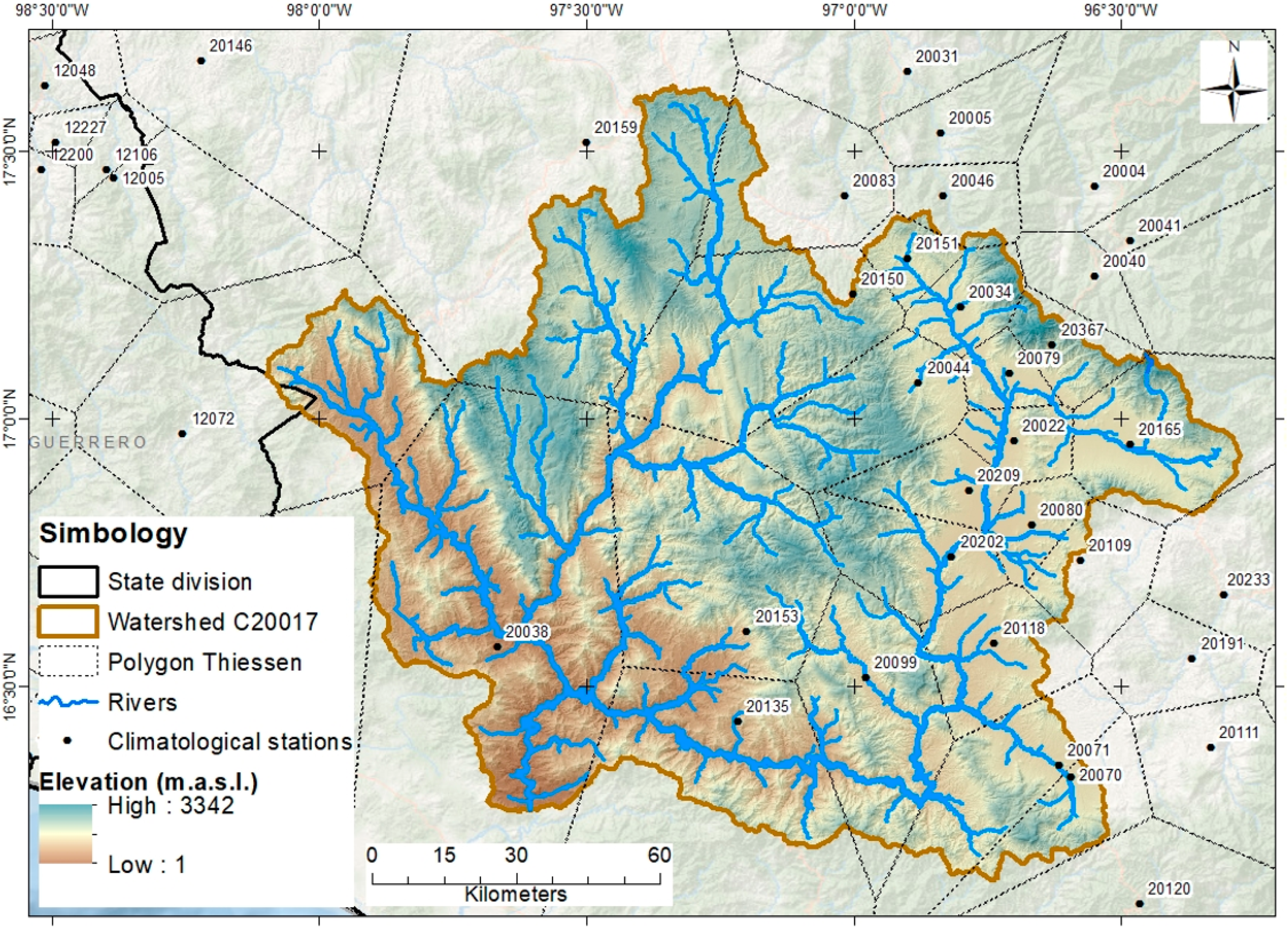
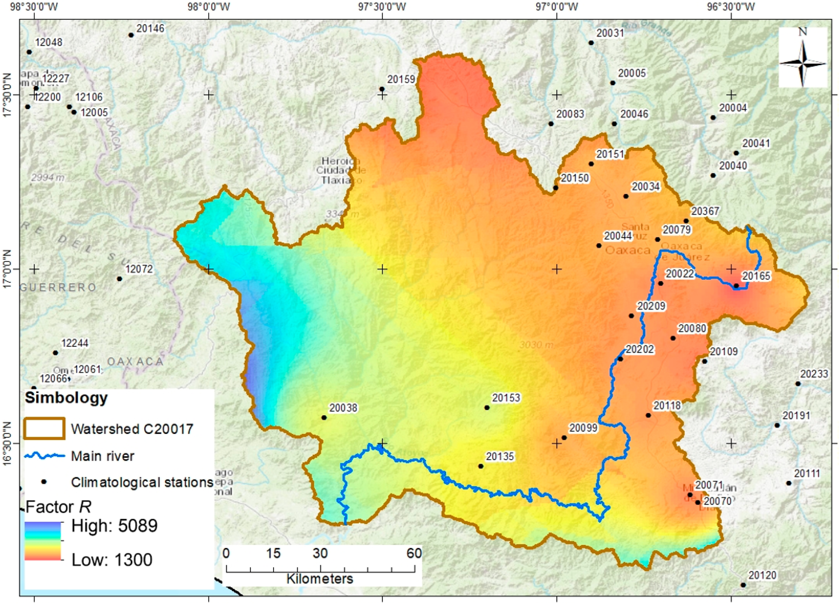
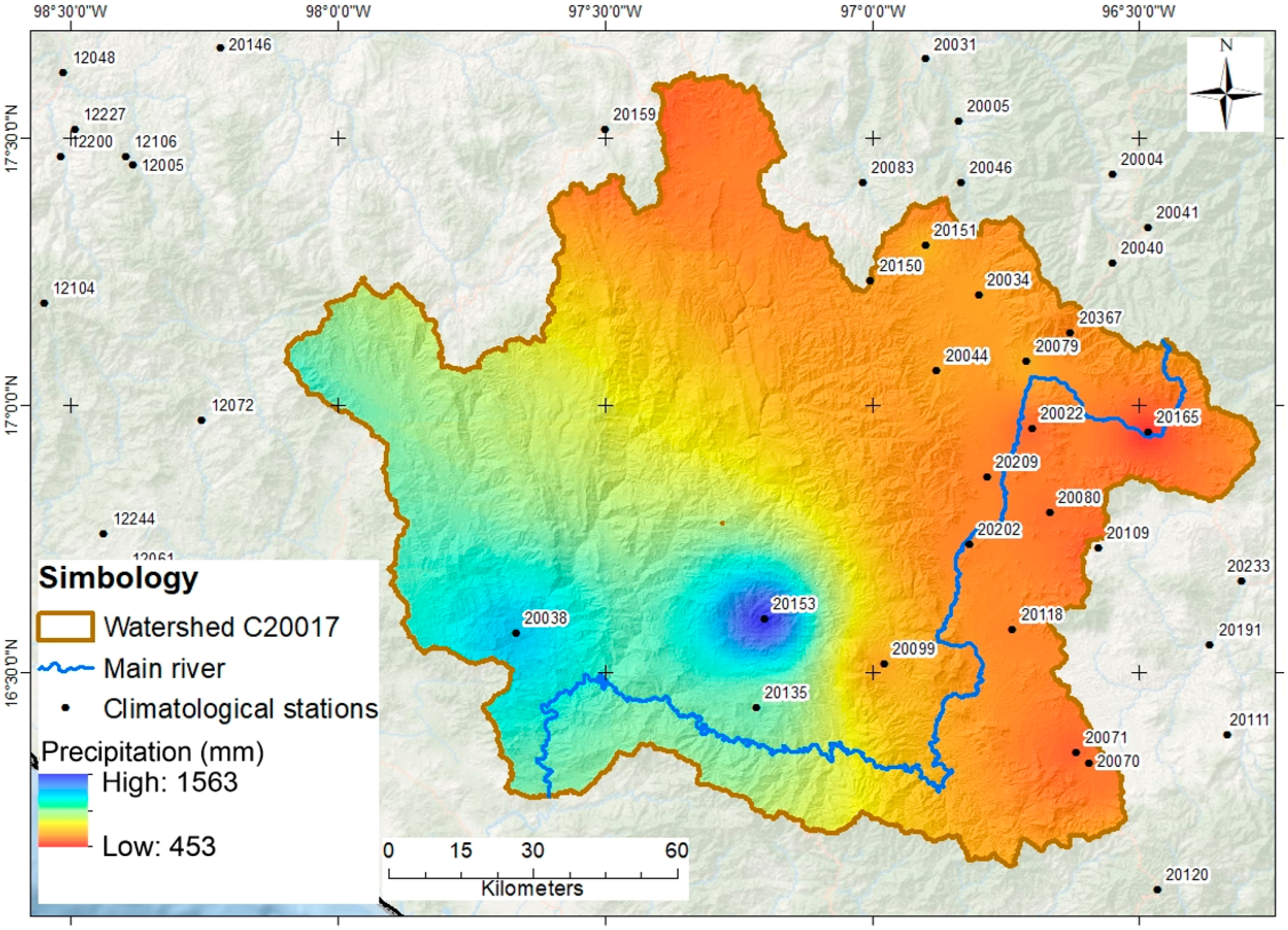
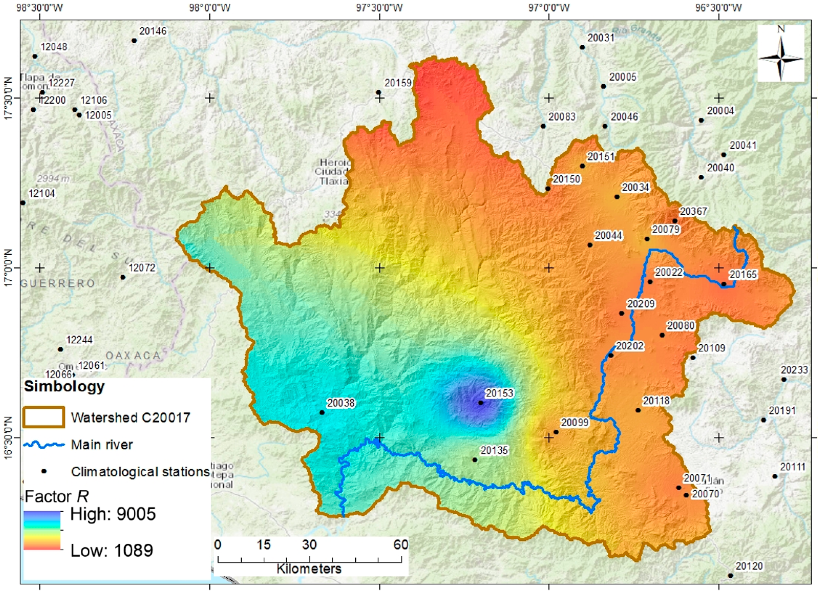
The basin-scale comparison carried out for the Paso de la Reyna watershed provides a useful qualitative illustration of these differences. In this example, the erosivity field obtained with the proposed methodology shows a spatial pattern that is broadly consistent with the distribution of mean annual rainfall, whereas the Cortes-based field appears smoother and less responsive to the internal contrasts evident in the basin. This result suggests that the daily rainfall-based approach captures the dominant gradients of erosive forcing in a physically plausible manner within the watershed. At the same time, the comparison should be interpreted as a basin-scale illustration rather than as a definitive proof of superiority for all applications.

An additional strength of the proposed methodology is the observational basis on which it was developed. Whereas the Cortes approach was derived from 53 stations, the present study relies on 170,796 storm events recorded at 432 Automatic Weather Stations, together with 2124 climatological stations used for national reconstruction. This broader information base does not eliminate uncertainty, but it improves the spatial representativeness of the analysis and provides a broader empirical basis for identifying regional contrasts in erosive forcing.

The results also have implications for current and future conservation planning. Because rainfall erosivity is a key climatic driver in USLE/RUSLE applications, improved estimation of R can support more reliable identification of erosion-prone areas, more realistic basin prioritization, and better targeting of preventive measures such as reforestation, cover management, slope protection, runoff regulation, and sediment-control practices. These implications become especially important under climate variability and climate change, since changes in storm intensity, rainfall concentration, and the frequency of erosive events may modify the erosive forcing acting on soils even where changes in annual rainfall totals are modest [3]. In that sense, the framework proposed here also provides a useful basis for future studies aimed at evaluating how rainfall erosivity may evolve under changing hydroclimatic conditions.

Finally, the present results should be interpreted not as a replacement for direct storm-based erosivity estimation wherever high-resolution rainfall records are available, but rather as an intermediate framework that expands erosivity assessment in data-constrained environments. In countries such as Mexico, where the density of daily rainfall data is much greater than the availability of long pluviographic series, this type of methodology can fill an important operational gap. The agreement between the national erosivity pattern and the known rainfall gradients of Mexico, together with the station-based and basin-scale comparisons presented here, suggests that the proposed approach provides a physically consistent basis for national-scale erosivity mapping in data-constrained environments.

Limitations and Future Work

Despite these encouraging results, several limitations should be acknowledged. First, the proposed methodology assumes that relationships derived from AWS storm records can be transferred to stations where only daily rainfall data are available. Although this transfer is physically reasonable and operationally useful, it may not fully capture local differences in storm structure, elevation effects, convective dynamics, orographic enhancement, and intrastorm intensity concentration. Second, missing daily rainfall values were infilled by inverse-distance weighting within previously defined homogeneous regions. This procedure improves record completeness and reduces inconsistencies associated with indiscriminate data transfer, but it still introduces uncertainty, particularly in areas with sparse station density or strong topographic contrasts.

Third, the analysis retained only storms with daily rainfall totals greater than 10 mm during the national calibration stage. This threshold is defensible from the standpoint of annual erosivity reconstruction because events below that magnitude usually contribute less to annual totals. However, it may exclude some short-duration, high-intensity storms capable of producing locally significant erosion, especially in highly vulnerable surfaces or small catchments. Fourth, the common analysis period of 1965–2006 does not explicitly capture more recent changes in rainfall extremes associated with climate variability and climate change. As a result, the present maps should be interpreted as representative of that reference period rather than as a direct depiction of current or future erosivity conditions.

A further point concerns validation. The national and basin-scale patterns obtained here are physically consistent with the rainfall gradients of Mexico and with the expected contrast between arid and humid regions, and the Cerro Catedral case study provides a direct quantitative comparison against storm-derived annual erosivity. Nevertheless, broader validation against additional long, independent sub-daily datasets would strengthen the assessment of predictive performance and help refine the transferability of the methodology across contrasting climatic regimes. Likewise, although IDW was selected for practical and operational reasons, a formal sensitivity analysis of interpolation parameters and benchmarking against alternative spatial predictors remain desirable.

Future work should therefore focus on four main directions. First, the uncertainty associated with data infilling and IDW-based interpolation should be quantified more explicitly, including sensitivity analyses in mountainous and data-sparse regions. Second, the methodology should be tested using updated pluviographic, radar-based, and satellite-supported rainfall datasets to evaluate its performance under more recent hydroclimatic conditions. Third, regionalization schemes based on climatic regime, elevation, or convective dominance could be explored to improve the transfer of the rainfall-erosivity relationship across Mexico. Fourth, the approach could be compared with alternative statistical and machine-learning methods for estimating storm erosivity from daily rainfall totals. Extending the framework to future climate scenarios would also provide a valuable basis for assessing how changes in rainfall erosivity may influence soil conservation needs, watershed management, and regional sustainability in coming decades.

5. Conclusions

This study developed a methodology for estimating the annual rainfall erosivity factor R from daily rainfall totals in Mexico using storm-scale information derived from 170,796 events recorded at 432 Automatic Weather Stations. On that basis, a four-parameter nonlinear relationship was established between daily rainfall depth and storm erosivity, and its parameters were subsequently transferred through spatial interpolation to 2124 climatological stations for the common period 1965–2006. This framework makes it possible to reconstruct annual rainfall erosivity from daily rainfall data while remaining consistent with the physical basis of the USLE/RUSLE erosivity concept.

The resulting national erosivity pattern reveals a clear contrast between the arid and semi-arid regions of northern and northwestern Mexico, where annual erosivity is generally low, and the humid to subhumid regions of central, southern, and southeastern Mexico, where erosivity is substantially higher. This spatial structure is consistent with the major hydroclimatic gradients of the country and indicates that the proposed methodology captures the dominant influence of rainfall amount, storm intensity, and rainfall concentration on erosive forcing. The results also show that erosivity varies appreciably within broad climatic regions, underscoring the importance of estimation methods capable of representing local and regional contrasts rather than relying exclusively on generalized regional equations.

The station-based comparison at the Cerro Catedral AWS showed that the proposed methodology reproduced the reference annual erosivity series derived from 10 min rainfall data more closely than the regional equations of Cortés, yielding a substantially smaller standard error of fit. In the Paso de la Reyna basin, the daily rainfall-based methodology also produced an erosivity field that was qualitatively consistent with the observed rainfall pattern. Together, these results support the usefulness of linking storm-scale erosivity information with the denser daily rainfall network, while broader quantitative benchmarking remains desirable.

The methodology presented here therefore contributes both a practical and a methodological advance. Practically, it expands the possibility of estimating rainfall erosivity in regions where sub-daily rainfall series are scarce but daily rainfall records are available. Methodologically, it provides a framework for transferring storm-based erosivity information to a national climatological network while preserving the main hydroclimatic gradients that control erosive forcing. These features make the proposed approach useful for subsequent applications involving soil-loss assessment, sediment-yield analysis, and watershed prioritization.

At the same time, the results should be interpreted within the limits of the available data and methods. In particular, the transferability of the rainfall-erosivity relationship, the uncertainty associated with data infilling and interpolation, the limited quantitative validation currently available, and the restriction to the period 1965–2006 indicate that further validation and updating are still desirable. Even so, the present study provides a practical and physically grounded basis for national scale erosivity assessment in Mexico and establishes a useful foundation for future improvements, including regional refinements, uncertainty analysis, and evaluation under changing climatic conditions.